
Method for Estimating Temporal Gait Parameters Concerning Bilateral Lower Limbs of Healthy Subjects Using a Single In-Shoe Motion Sensor through a Gait Event Detection Approach

 ,
,
Abstract
:
1. Introduction
2. Materials and Methods
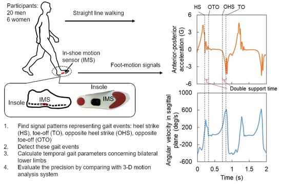
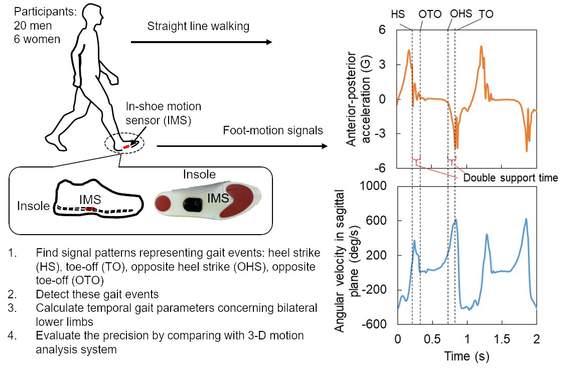
2.1. Participants
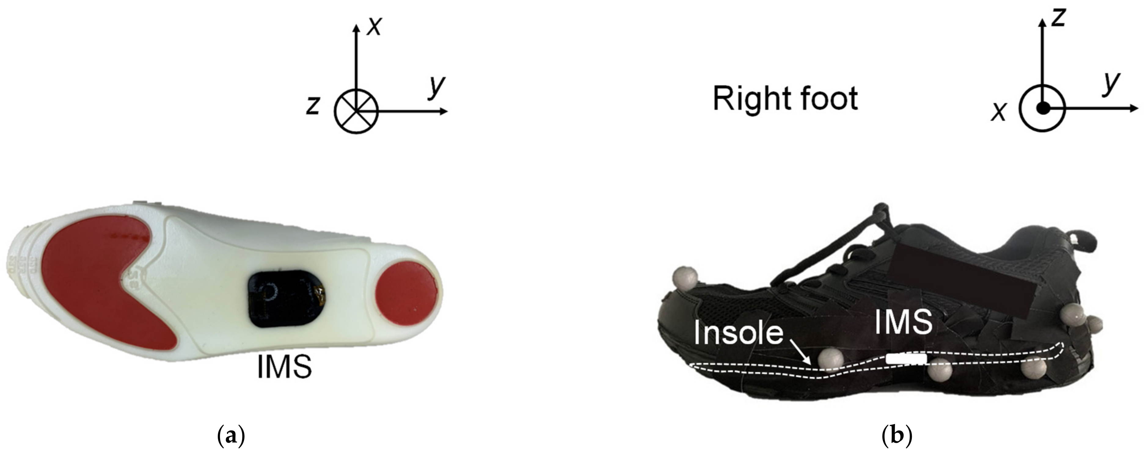
2.2. Experimental Setup
2.3. Experimental Protocol
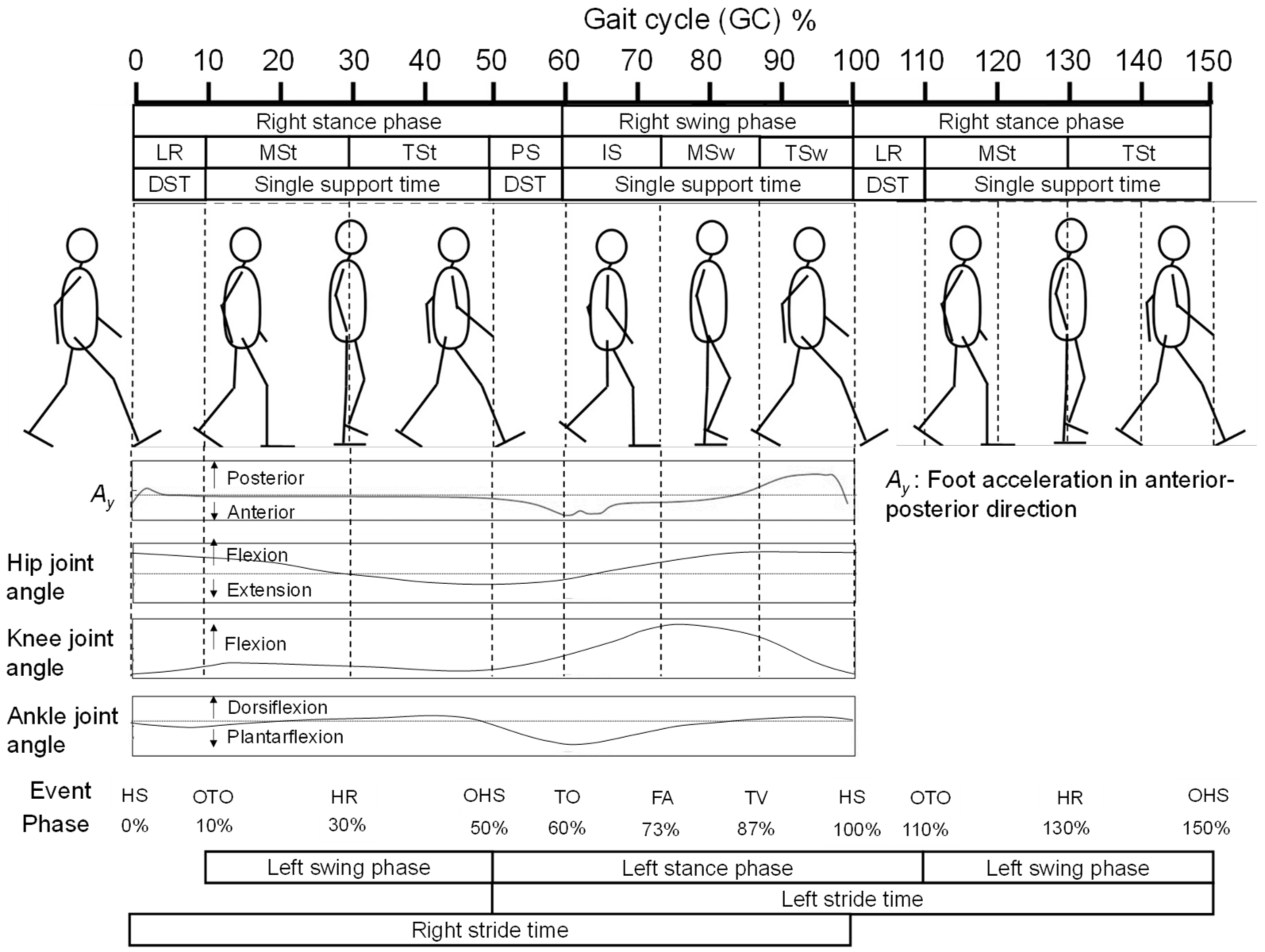
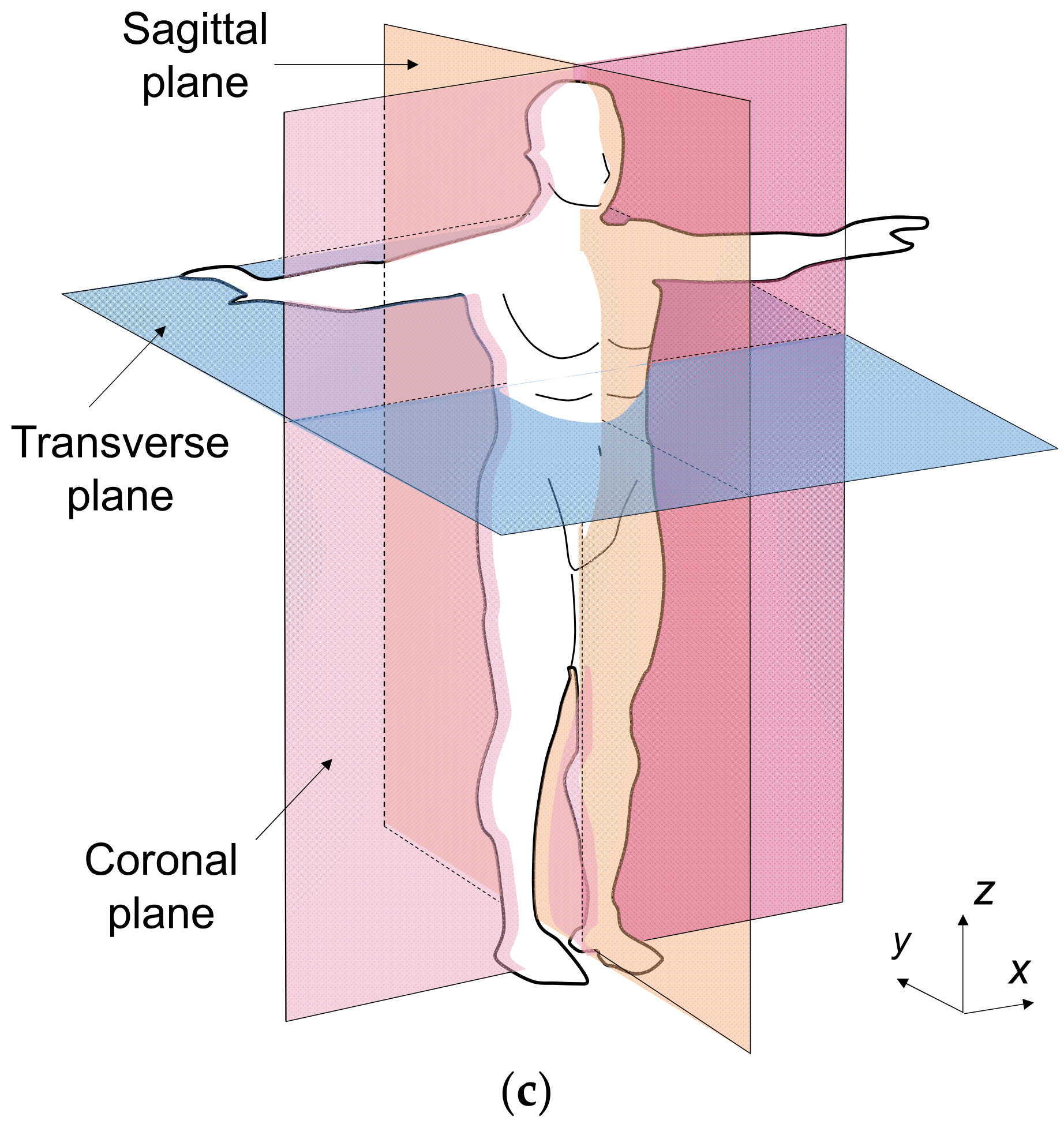
2.4. Feature Selection for OHS and OTO Detection from Foot Motion through Biomechanical Analysis
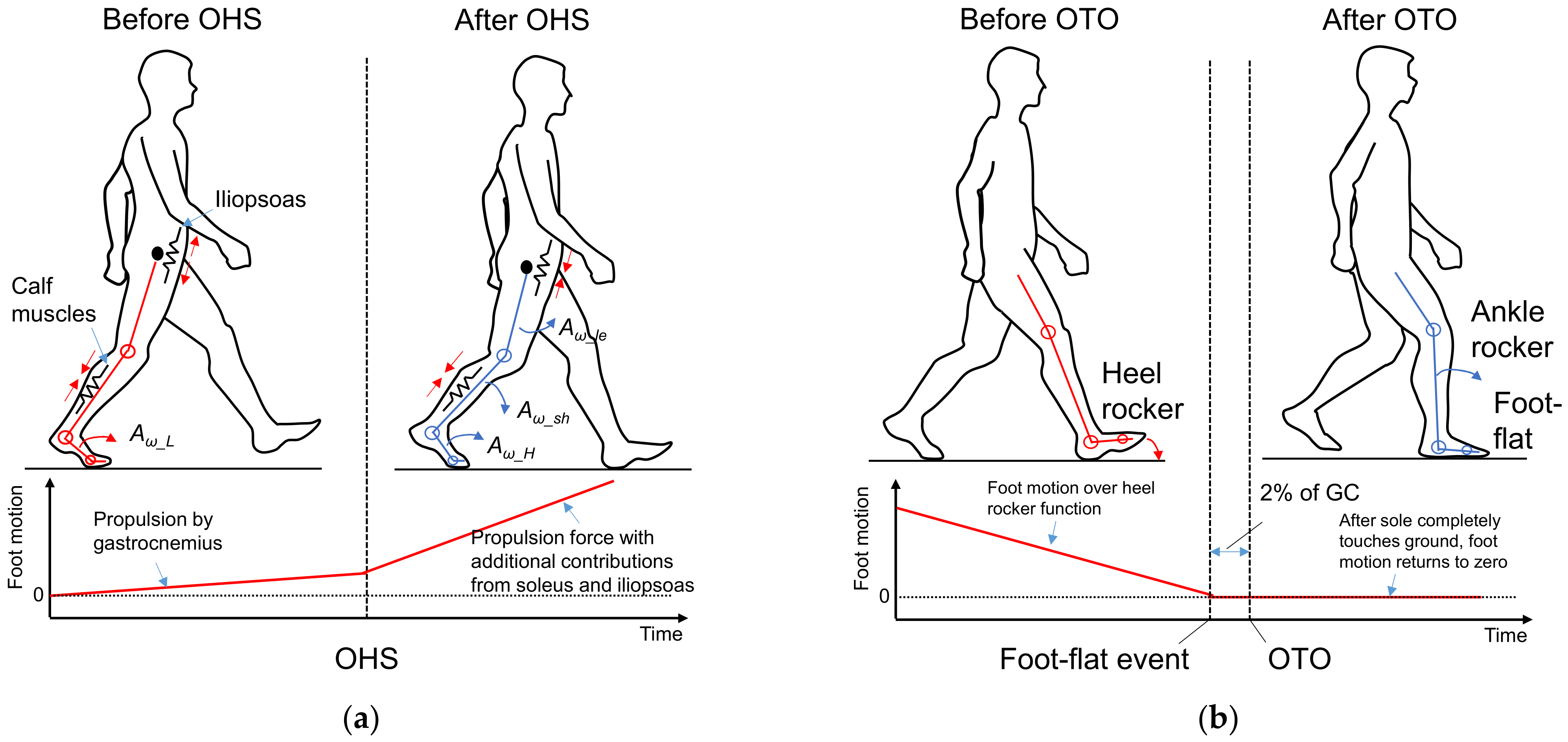
2.4.1. Foot Motion near OHS
2.4.2. Foot Motion near OTO
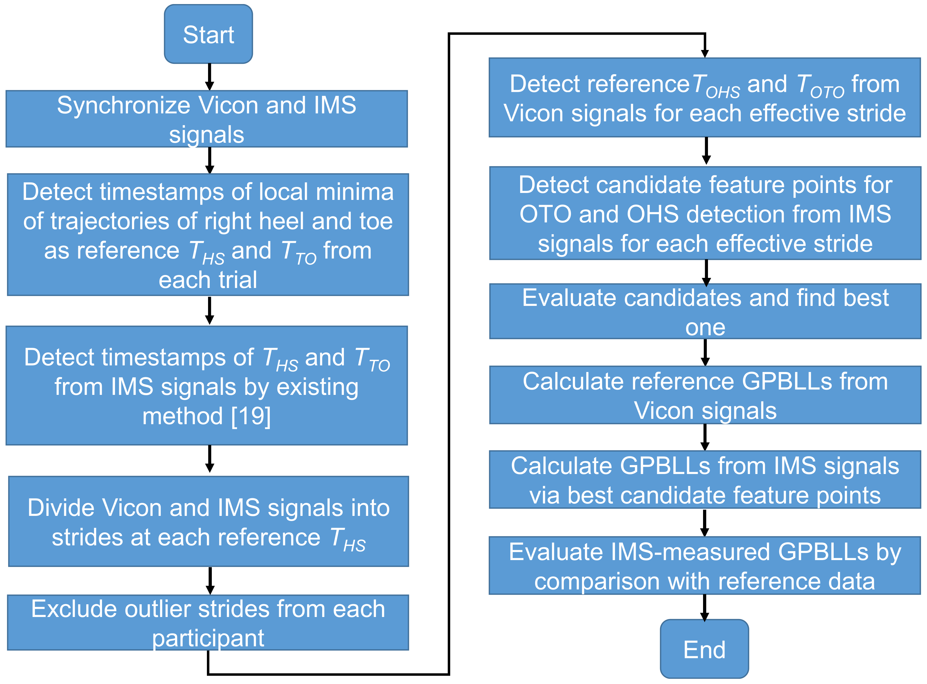
2.5. Data Processing for Analysis
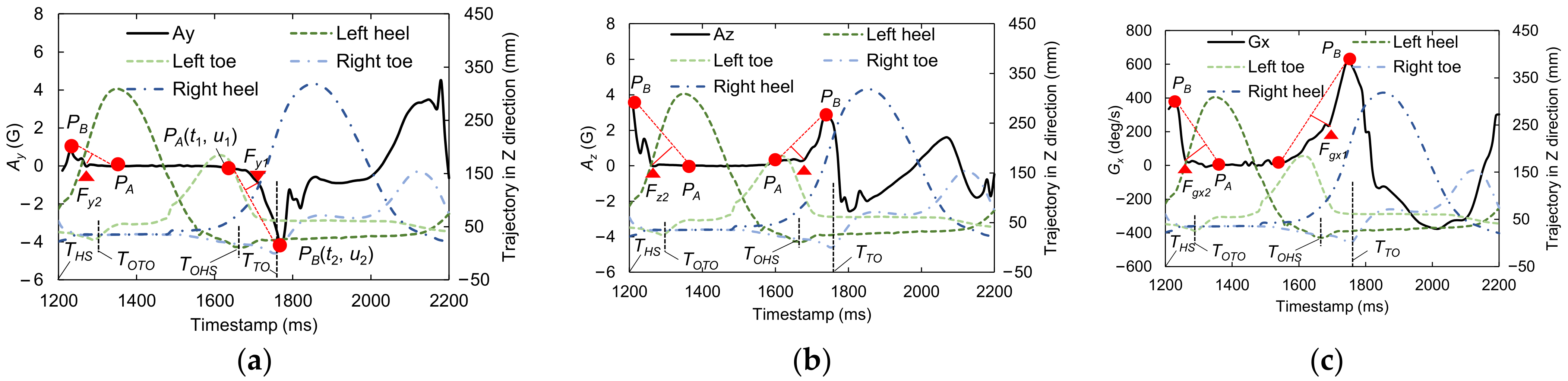
2.6. Candidate Feature Points for OHS and OTO Detection
2.7. Temporal GPBLL Estimation through Gait Event Detection Approach
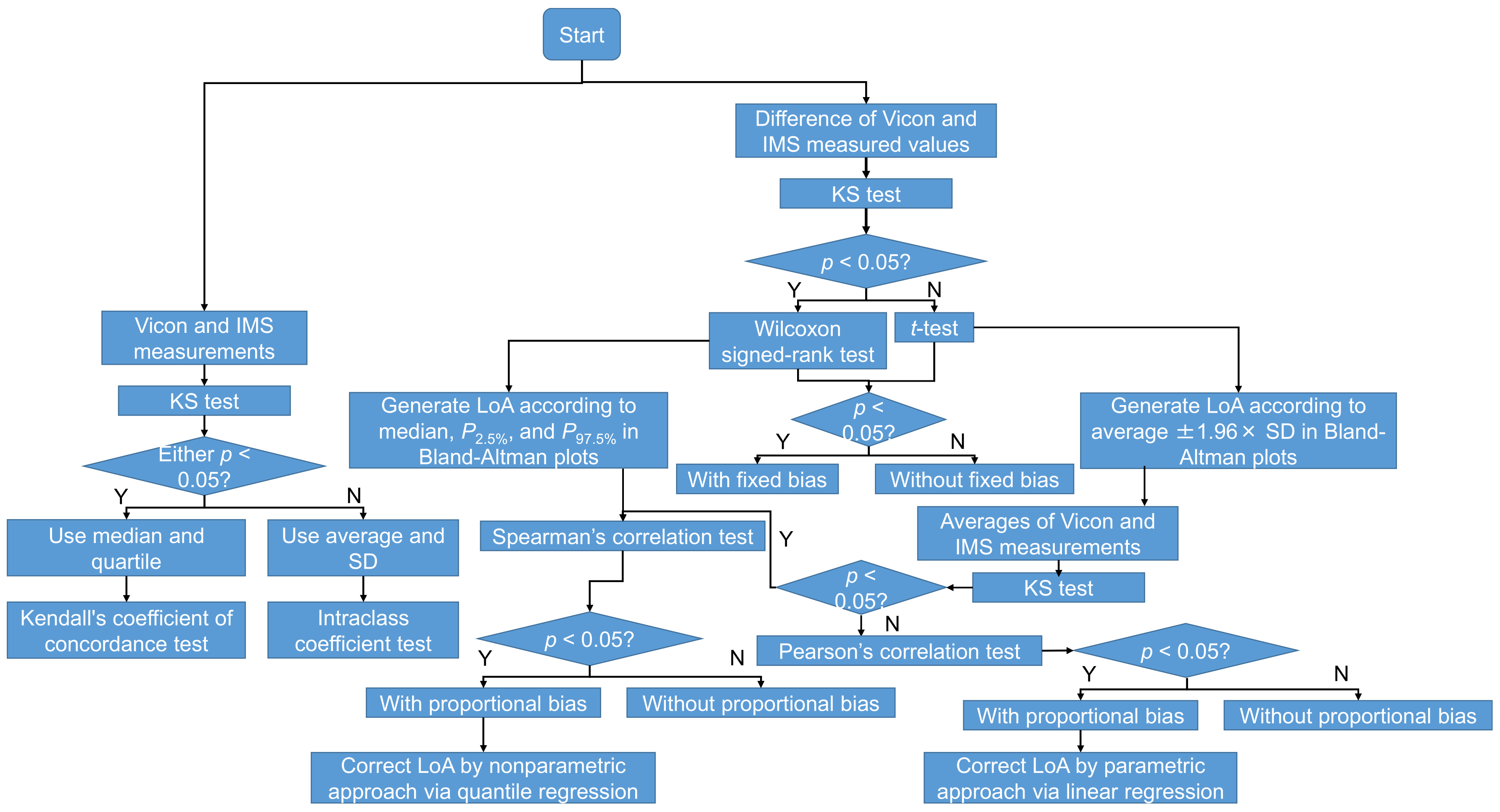
2.8. Statistical Analysis
3. Results
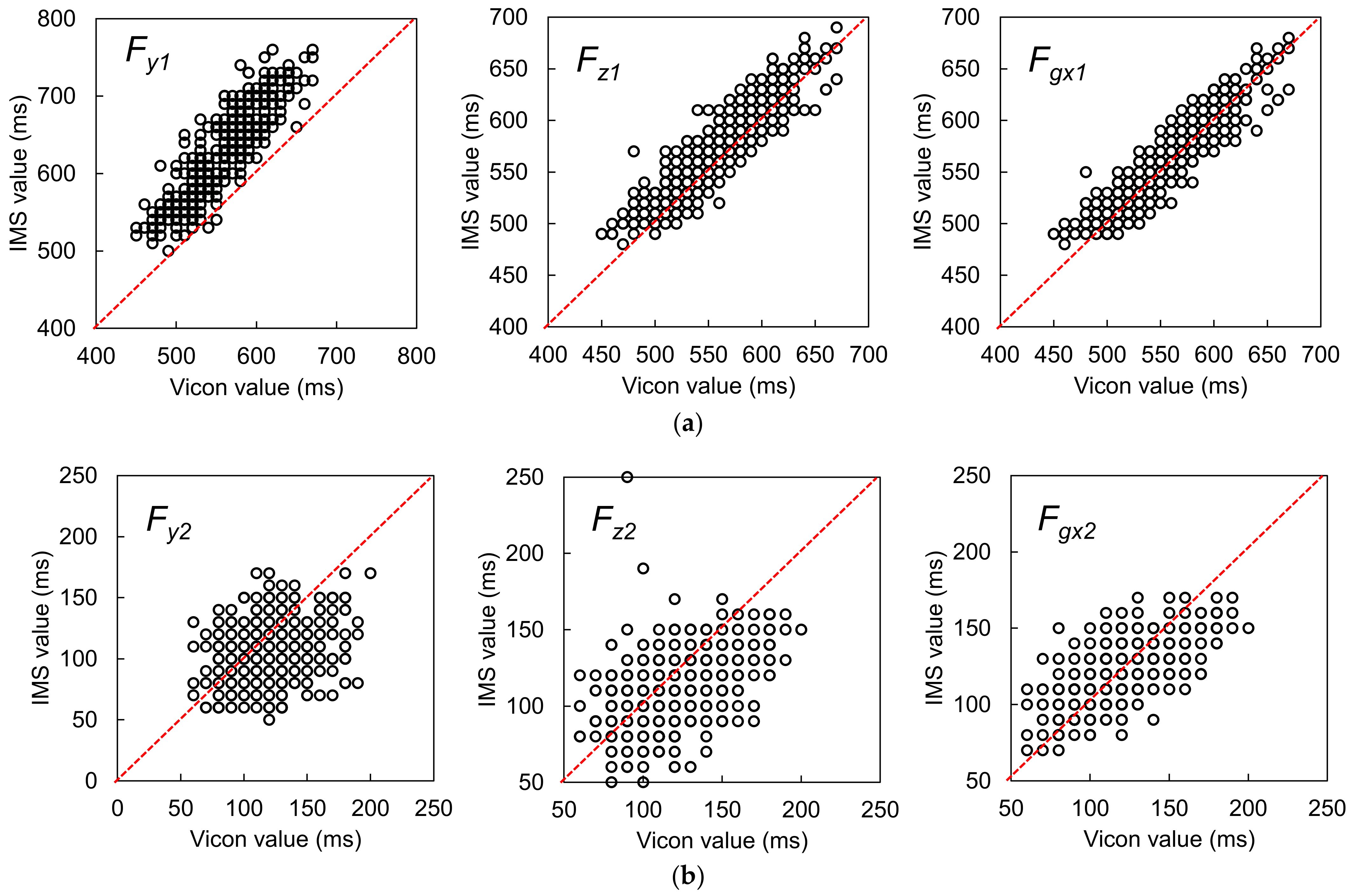
3.1. Evaluation of Signal Features for Gait Event Detection
3.1.1. Best Candidate Signal Feature for OHS Detection
3.1.2. Best Candidate Signal Feature for OTO Detection
3.2. Evaluation of Using GPBLL Measurements for Gait Event Detection
3.2.1. Results for One-Stride Measurement
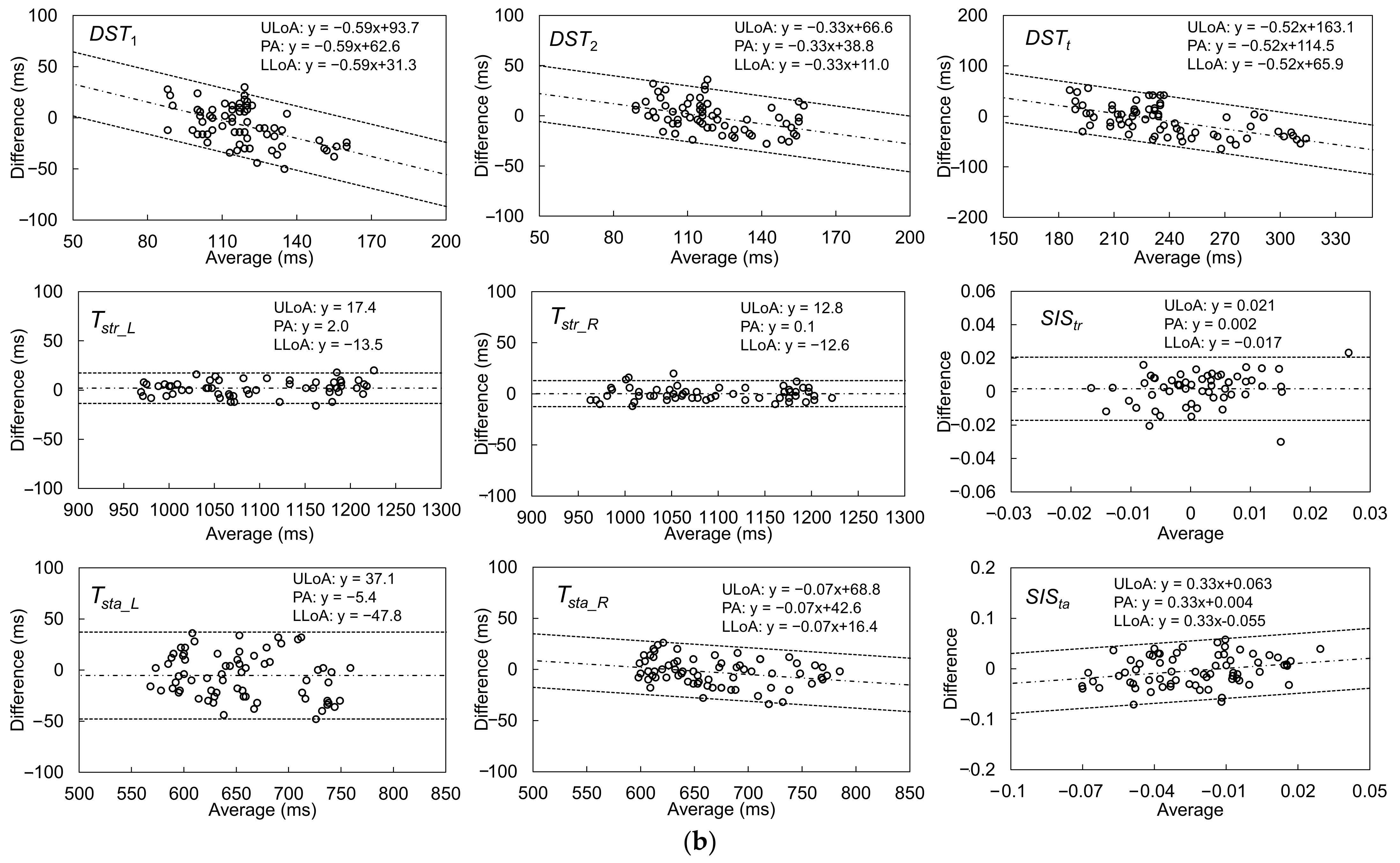
3.2.2. Results for Multiple-Stride Measurement
4. Discussion
5. Conclusions
Supplementary Materials
Author Contributions
Funding
Institutional Review Board Statement
Informed Consent Statement
Acknowledgments
Conflicts of Interest
References
- Rast, F.M.; Labruyère, R. Systematic review on the application of wearable inertial sensors to quantify everyday life motor activity in people with mobility impairments. J. NeuroEng. Rehabil. 2020, 17, 148. [Google Scholar] [CrossRef]
- Jagos, H.; Pils, K.; Haller, M.; Wassermann, C.; Chhatwal, C.; Rafolt, D.; Rattay, F. Mobile gait analysis via eSHOEs instrumented shoe insoles: A pilot study for validation against the gold standard GAITRite®. J. Med. Eng. Technol. 2017, 41, 375–386. [Google Scholar] [CrossRef]
- Gokalgandhi, D.; Kamdar, L.; Shah, N.; Mehendale, N. A Review of Smart Technologies Embedded in Shoes. J. Med. Syst. 2020, 44, 150. [Google Scholar] [CrossRef]
- Eskofier, B.M.; Lee, S.I.; Baron, M.; Simon, A.; Martindale, C.F.; Gaßner, H.; Klucken, J. An overview of smart shoes in the internet of health things: Gait and mobility assessment in health promotion and disease monitoring. Appl. Sci. 2017, 7, 986. [Google Scholar] [CrossRef] [Green Version]
- Mariani, B.; Rochat, S.; Büla, C.J.; Aminian, K. Heel and toe clearance estimation for gait analysis using wireless inertial sensors. IEEE Trans. Biomed. Eng. 2012, 59, 3162–3168. [Google Scholar] [CrossRef]
- Ellis, R.G.; Howard, K.C.; Kram, R. The metabolic and mechanical costs of step time asymmetry in walking. Proc. R. Soc. B-Biol. Sci. 2013, 280, 20122784. [Google Scholar] [CrossRef] [PubMed] [Green Version]
- Zhang, G.; Wong, D.W.-C.; Wong, I.K.-K.; Chen, T.L.-W.; Hong, T.T.-H.; Peng, Y.; Wang, Y.; Tan, Q.; Zhang, M. Plantar Pressure Variability and Asymmetry in Elderly Performing 60-Minute Treadmill Brisk-Walking: Paving the Way towards Fatigue-Induced Instability Assessment Using Wearable In-Shoe Pressure Sensors. Sensors 2021, 21, 3217. [Google Scholar] [CrossRef]
- Park, E.; Lee, S.I.; Nam, H.S.; Garst, J.H.; Huang, A.; Campion, A.; Arnell, M.; Ghalehsariand, N.; Park, S.S.; Chang, H.J.; et al. Unobtrusive and continuous monitoring of alcohol-impaired gait using smart shoes. Methods Inf. Med. 2017, 56, 74–82. [Google Scholar] [CrossRef] [PubMed] [Green Version]
- Scarborough, D.M.; Krebs, D.E.; Harris, B.A. Quadriceps muscle strength and dynamic stability in elderly persons. Gait Posture 1999, 10, 10–20. [Google Scholar] [CrossRef]
- Taylor, M.E.; Delbaere, K.; Mikolaizak, A.S.; Lord, S.R.; Close, J.C. Gait parameter risk factors for falls under simple and dual task conditions in cognitively impaired older people. Gait Posture 2013, 37, 126–130. [Google Scholar] [CrossRef]
- Kim, C.M.; Eng, J.J. Symmetry in vertical ground reaction force is accompanied by symmetry in temporal but not distance variables of gait in persons with stroke. Gait Posture 2003, 18, 23–28. [Google Scholar] [CrossRef]
- Nagano, H.; James, L.; Sparrow, W.A.; Begg, R.K. Effects of walking-induced fatigue on gait function and tripping risks in older adults. J. NeuroEng. Rehabil. 2014, 11, 155. [Google Scholar] [CrossRef] [PubMed] [Green Version]
- Anwary, A.R.; Yu, H.; Vassallo, M. An Automatic Gait Feature Extraction Method for Identifying Gait Asymmetry Using Wearable Sensors. Sensors 2018, 18, 676. [Google Scholar] [CrossRef] [PubMed] [Green Version]
- Han, S.H.; Kim, C.O.; Kim, K.J.; Jeon, J.; Chang, H.; Kim, E.S.; Park, H. Quantitative analysis of the bilateral coordination and gait asymmetry using inertial measurement unit-based gait analysis. PLoS ONE 2019, 14, e0222913. [Google Scholar] [CrossRef] [PubMed] [Green Version]
- Rhee, I.K.; Lee, J.; Kim, J.; Serpedin, E.; Wu, Y.C. Clock Synchronization in Wireless Sensor Networks: An Overview. Sensors 2009, 9, 56–85. [Google Scholar] [CrossRef] [PubMed] [Green Version]
- Sichitiu, M.L.; Veerarittiphan, C. Simple, accurate time synchronization for wireless sensor networks. In In Proceedings of the 2003 IEEE Wireless Communications and Networking, New Orleans, LA, USA, 16–20 March 2003; Volume 2, pp. 1266–1273. [Google Scholar] [CrossRef]
- Neumann, D.A. Kinesiology of the Musculoskeletal System: Foundations of Physical Rehabilitation, 2nd ed.; Mosby: St Louis, MO, USA, 2010; pp. 627–676. [Google Scholar]
- Huang, C.; Fukushi, K.; Wang, Z.; Kajitani, H.; Nihey, F.; Nakahara, K. Initial Contact and Toe-Off Event Detection Method for In-Shoe Motion Sensor. In Activity and Behavior Computing. Smart Innovation, Systems and Technologies; Ahad, M.A.R., Inoue, S., Roggen, D., Fujinami, K., Eds.; Springer: Singapore, 2021; Volume 204. [Google Scholar] [CrossRef]
- Caldas, R.; Mundt, M.; Potthast, W.; de Lima Neto, F.B.; Markert, B. A systematic review of gait analysis methods based on inertial sensors and adaptive algorithms. Gait Posture 2017, 57, 204–210. [Google Scholar] [CrossRef] [PubMed]
- Taborri, J.; Palermo, E.; Rossi, S.; Cappa, P. Gait Partitioning Methods: A Systematic Review. Sensors 2016, 16, 66. [Google Scholar] [CrossRef] [Green Version]
- González, I.; Fontecha, J.; Hervás, R.; Bravo, J. An Ambulatory System for Gait Monitoring Based on Wireless Sensorized Insoles. Sensors 2015, 15, 16589–16613. [Google Scholar] [CrossRef] [Green Version]
- Liu, T.; Inoue, Y.; Shibata, K. Development of a wearable sensor system for quantitative gait analysis. Measurement 2009, 42, 978–988. [Google Scholar] [CrossRef]
- Mannini, A.; Genovese, V.; Sabatini, A.M. Online decoding of hidden Markov models for gait event detection using foot-mounted gyroscopes. IEEE J. Biomed. Health 2013, 18, 1122–1130. [Google Scholar] [CrossRef]
- Kidziński, Ł.; Delp, S.; Schwartz, M. Automatic real-time gait event detection in children using deep neural networks. PLoS ONE 2019, 14, e0211466. [Google Scholar] [CrossRef] [PubMed] [Green Version]
- Rueterbories, J.; Spaich, E.G.; Andersen, O.K. Gait event detection for use in FES rehabilitation by radial and tangential foot accelerations. Med. Eng. Phys. 2014, 36, 502–508. [Google Scholar] [CrossRef] [PubMed]
- Endo, K.; Herr, H. Human walking model predicts joint mechanics, electromyography and mechanical economy. In Proceedings of the 2009 IEEE/RSJ International Conference on Intelligent Robots and Systems, St. Louis, MO, USA, 10–15 October 2009; pp. 4663–4668. [Google Scholar] [CrossRef]
- Madgwick, S.O.H.; Harrison, A.J.L.; Vaidyanathan, R. Estimation of IMU and MARG orientation using a gradient descent algorithm. In Proceedings of the 2011 IEEE International Conference on Rehabilitation Robotics, Zurich, Switzerland, 29 June–1 July 2011; pp. 1–7. [Google Scholar] [CrossRef]
- Houglum, P.A.; Bertoti, D.B. Brunnstrom’s Clinical Kinesiology, 6th ed.; FA Davis: Philadelphia, PA, USA, 2011; pp. 533–585. [Google Scholar]
- Perry, J. Gait Analysis: Normal and Pathological Function, 2nd ed.; Slack: Thorofare, NJ, USA, 2010; pp. 19–46. [Google Scholar]
- Sangeux, M.; Polak, J. A simple method to choose the most representative stride and detect outliers. Gait Posture 2015, 41, 726–730. [Google Scholar] [CrossRef] [PubMed]
- Nilufar, S.; Morrow, A.A.; Lee, J.M.; Perkins, T.J. FiloDetect: Automatic detection of filopodia from fluorescence microscopy images. BMC Syst. Biol. 2013, 7, 66. [Google Scholar] [CrossRef] [Green Version]
- Bland, J.M.; Altman, D. Statistical methods for assessing agreement between two methods of clinical measurement. Lancet 1986, 327, 307–310. [Google Scholar] [CrossRef]
- Bland, J.M.; Altman, D.G. Measuring agreement in method comparison studies. Stat. Methods Med. Res. 1999, 8, 135–160. [Google Scholar] [CrossRef]
- Chen, L.A.; Kao, C.L. Parametric and nonparametric improvements in Bland and Altman’s assessment of agreement method. Stat. Med. 2021, 40, 2155–2176. [Google Scholar] [CrossRef]
- Cicchetti, D.V. Guidelines, criteria, and rules of thumb for evaluating normed and standardized assessment instruments in psychology. Psychol. Assess. 1994, 6, 284. [Google Scholar] [CrossRef]
- Moslem, S.; Ghorbanzadeh, O.; Blaschke, T.; Duleba, S. Analysing stakeholder consensus for a sustainable transport development decision by the fuzzy AHP and interval AHP. Sustainability 2019, 11, 3271. [Google Scholar] [CrossRef] [Green Version]
- Wilson, C.M.; Kostsuca, S.R.; Boura, J.A. Utilization of a 5-meter walk test in evaluating self-selected gait speed during preoperative screening of patients scheduled for cardiac surgery. Cardiopulm. Phys. Ther. J. 2013, 24, 36. [Google Scholar] [CrossRef]
- Kirtley, C.; Whittle, M.W.; Jefferson, R.J. Influence of walking speed on gait parameters. J. Biomed. Eng. 1985, 7, 282–288. [Google Scholar] [CrossRef]
- Kaczmarczyk, K.; Błażkiewicz, M.; Wit, A.; Wychowański, M. Assessing the asymmetry of free gait in healthy young subjects. Acta Bioeng. Biomech. 2017, 19, 101–106. [Google Scholar] [CrossRef] [PubMed]
- Lai, P.P.; Leung, A.K.; Li, A.N.; Zhang, M. Three-dimensional gait analysis of obese adults. Clin. Biomech. 2008, 23, S2–S6. [Google Scholar] [CrossRef]
- Montero-Odasso, M.; Casas, A.; Hansen, K.T.; Bilski, P.; Gutmanis, I.; Wells, J.L.; Borrie, M.J. Quantitative gait analysis under dual-task in older people with mild cognitive impairment: A reliability study. J. Neuroeng. Rehabil. 2009, 6, 35. [Google Scholar] [CrossRef] [PubMed] [Green Version]
- Lemke, M.R.; Wendorff, T.; Mieth, B.; Buhl, K.; Linnemann, M. Spatiotemporal gait patterns during over ground locomotion in major depression compared with healthy controls. J. Psychiat. Res. 2000, 34, 277–283. [Google Scholar] [CrossRef]
- Lobet, S.; Hermans, C.; Bastien, G.J.; Massaad, F.; Detrembleur, C. Impact of ankle osteoarthritis on the energetics and mechanics of gait: The case of hemophilic arthropathy. Clin. Biomech. 2012, 27, 625–631. [Google Scholar] [CrossRef] [PubMed]
- Wiszomirska, I.; Błażkiewicz, M.; Kaczmarczyk, K.; Brzuszkiewicz-Kuźmicka, G.; Wit, A. Effect of drop foot on spatiotemporal, kinematic, and kinetic parameters during gait. Appl. Bionics Biomech. 2017, 2017, 3595461. [Google Scholar] [CrossRef]
- Boudarham, J.; Roche, N.; Pradon, D.; Bonnyaud, C.; Bensmail, D.; Zory, R. Variations in kinematics during clinical gait analysis in stroke patients. PLoS ONE 2013, 8, e66421. [Google Scholar] [CrossRef]


| Gait Event | Feature | Relative Time to HS (ms) | Temporal Difference (ms) | Kendall’s W | ||||
|---|---|---|---|---|---|---|---|---|
| Vicon (Median (Lower–Upper Quartile)) | IMS (Median (Lower–Upper Quartile)) | Accuracy (Median) | Precision (QD) | Fixed Bias? (p-Value) | Proportional Bias? (r, p-Value) | |||
| OHS | Fy1 | 550 (520–590) | 620 (570–670) | 60 | 20 | p < 0.001 | r = 0.279, p < 0.001 | 0.943 |
| Fz1 | 570 (530–605) | 10 | 15 | p < 0.001 | r = 0.095, p = 0.028 | 0.963 | ||
| Fgx1 | 560 (520–590) | 0 | 15 | p < 0.001 | r = −0.022, p = 0.614 | 0.966 | ||
| OTO | Fy2 + 2%GC | 120 (100–140) | 110 (90–120) | −10 | 20 | p < 0.001 | r = −0.049, p = 0.250 | 0.618 |
| Fz2 + 2%GC | 110 (100–130) | −10 | 20 | p < 0.001 | r = −0.589, p < 0.001 | 0.727 | ||
| Fgx2 + 2%GC | 120 (110–130) | 0 | 10 | p = 0.151 | r = −0.372, p < 0.001 | 0.837 | ||
| Gait Parameter | Median (Lower–Upper Quartile) | Temporal Difference | Kendall’s W | |||
|---|---|---|---|---|---|---|
| Vicon (ms) | IMS (ms) | Accuracy and Precision (Median (QD), ms) | Fixed Bias? (p-Value) | Proportional Bias? (r, p-Value) | ||
| DST1 (ms) | 120 (107.5–140) | 110 (100–130) | −10 (15) | Y p < 0.001 | r = −0.279, p < 0.001 | 0.687 |
| DST2 (ms) | 120 (110–140) | 120 (110–130) | 0 (10) | N p = 0.608 | r = −0.410, p < 0.001 | 0.814 |
| DSTt (ms) | 240 (210–270) | 230 (210–250) | 0 (25) | Y p < 0.001 | r = −0.485, p < 0.001 | 0.794 |
| Tstr_L (ms) | 1080 (1020–1170) | 1070 (1020–1160) | 0 (10) | N p = 0.529 | r = 0.033, p = 0.549 | 0.985 |
| Tstr_R (ms) | 1070 (1020–1160) | 1070 (1020–1160) | 0 (10) | N p = 0.612 | r = 0.069, p = 0.206 | 0.988 |
| Tsta_L (ms) | 650 (600–690) | 640 (610–690) | 0 (20) | Y p = 0.032 | r = −0.182, p < 0.001 | 0.925 |
| Tsta_R (ms) | 665 (620–710) | 665 (620–700) | 0 (15) | Y p = 0.022 | r = −0.172, p < 0.001 | 0.967 |
| SIStr | 0.000 (−0.011–0.010) | 0.000 (−0.017–0.017) | 0.000 (0.014) | N p = 0.379 | r = 0.250, p < 0.001 | 0.698 |
| SISta | −0.017 (−0.046–0.000) | −0.026 (−0.060–0.014) | 0.000 (0.032) | N p = 0.708 | r = 0.359, p < 0.001 | 0.708 |
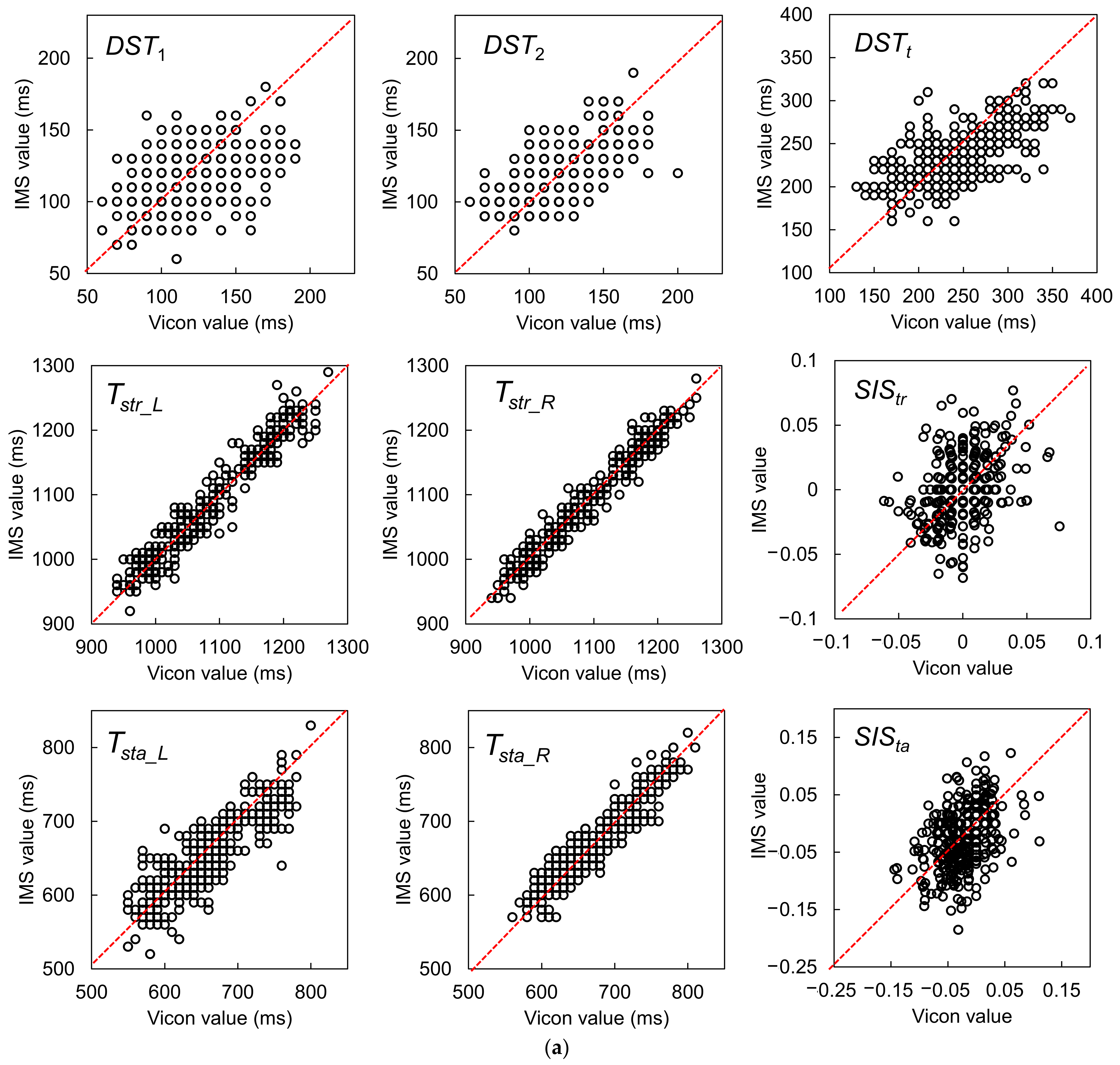
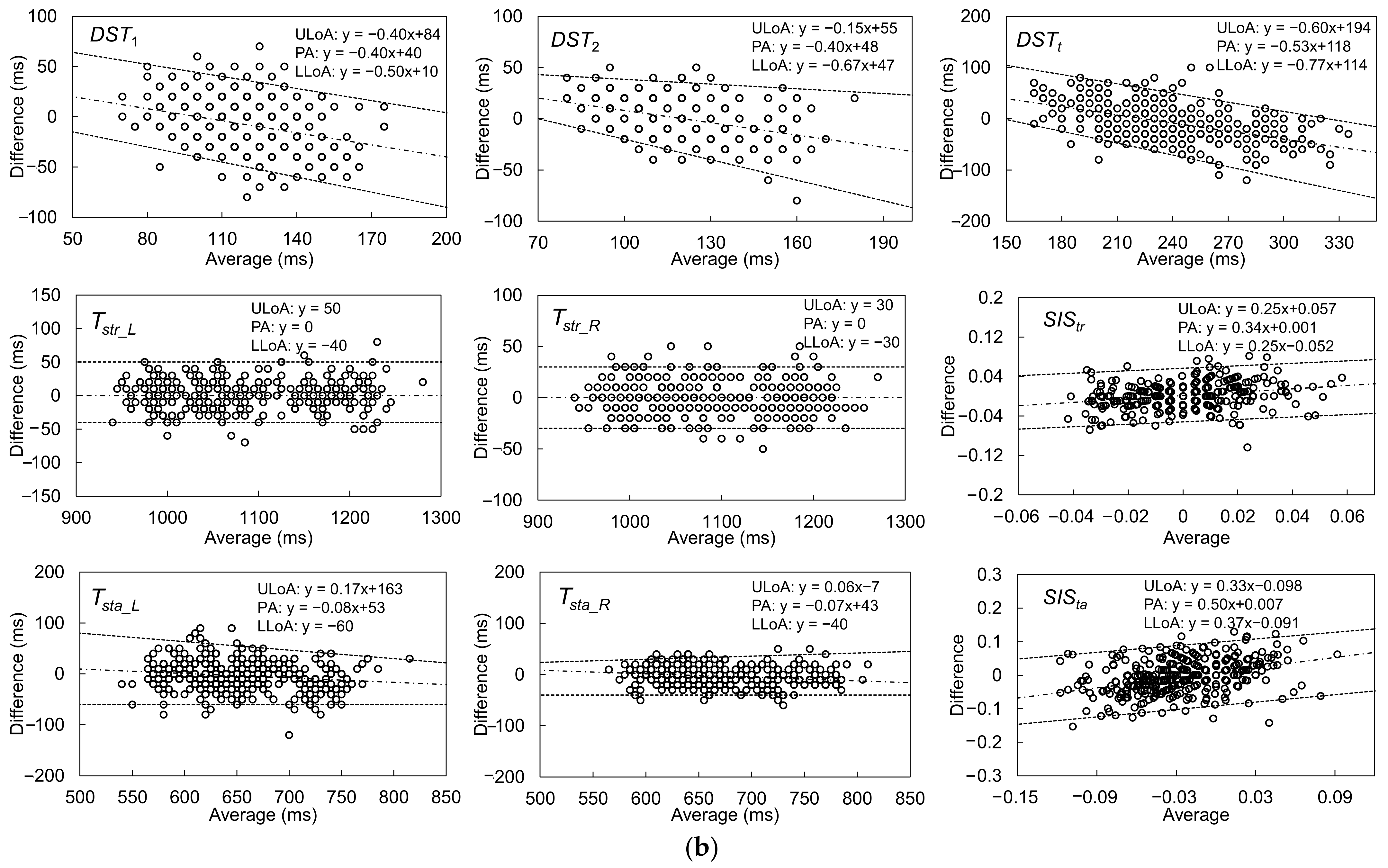
| Gait Parameter | Accuracy (Average, ms) | Precision (SD, ms) | Fixed Bias? (p-Value) | Proportional Bias? (r, p-Value) | ICC(2,k) |
|---|---|---|---|---|---|
| DST1 (ms) | −6.9 | 18.9 | Y p = 0.003 | r = −0.530, p = <0.001 | 0.665 |
| DST2 (ms) | −1.3 | 15.4 | N p = 0.493 | r = −0.410, p = <0.001 | 0.835 |
| DSTt (ms) | −8.2 | 30.1 | Y p = 0.027 | r = −0.596, p = <0.001 | 0.800 |
| Tstr_L (ms) | 2.0 | 8.0 | N p = 0.707 | r = 0.160, p = 0.238 | 0.998 |
| Tstr_R (ms) | 0.1 | 6.5 | N p = 0.935 | r = −0.024, p = 0.864 | 0.998 |
| Tsta_L (ms) | −5.4 | 21.8 | Y p = 0.045 | r = −0.216, p = 0.075 | 0.957 |
| Tsta_R (ms) | −2.8 | 13.3 | N p = 0.081 | r = −0.273, p = 0.023 | 0.984 |
| SIStr | 0.002 | 0.010 | N p = 0.186 | r = 0.250, p = 0.063 | 0.654 |
| SISta | −0.004 | 0.030 | N p = 0.297 | r = 0.263, p = 0.029 | 0.602 |
| Potential Application | Gait Parameter | Required Precision | Achieved Precision | Reference |
|---|---|---|---|---|
| Fall | DSTtotal | 80 ms | 18.9 ms | [10] |
| Fatigue | DSTtotal | 2.00%GC or 17–26 ms | 18.9 ms | [12] |
| Obesity | Tsta_L or Tsta_R | 1.70%GC or 15–24 ms | 8.0 or 6.5 ms | [40] |
| DSTtotal | 3.48%GC or 30–45 ms | 18.9 ms | ||
| Mild cognitive impairment | DSTtotal | 30 ms | 18.9 ms | [41] |
| Depression | DSTtotal | 54 ms | 18.9 ms | [42] |
| Tsta_L or Tsta_L | 65 ms | 8.0 or 6.5 ms |
Publisher’s Note: MDPI stays neutral with regard to jurisdictional claims in published maps and institutional affiliations. |
© 2022 by the authors. Licensee MDPI, Basel, Switzerland. This article is an open access article distributed under the terms and conditions of the Creative Commons Attribution (CC BY) license (https://creativecommons.org/licenses/by/4.0/).
Share and Cite
Huang, C.; Fukushi, K.; Wang, Z.; Nihey, F.; Kajitani, H.; Nakahara, K. Method for Estimating Temporal Gait Parameters Concerning Bilateral Lower Limbs of Healthy Subjects Using a Single In-Shoe Motion Sensor through a Gait Event Detection Approach. Sensors 2022, 22, 351. https://doi.org/10.3390/s22010351
Huang C, Fukushi K, Wang Z, Nihey F, Kajitani H, Nakahara K. Method for Estimating Temporal Gait Parameters Concerning Bilateral Lower Limbs of Healthy Subjects Using a Single In-Shoe Motion Sensor through a Gait Event Detection Approach. Sensors. 2022; 22(1):351. https://doi.org/10.3390/s22010351
Chicago/Turabian StyleHuang, Chenhui, Kenichiro Fukushi, Zhenwei Wang, Fumiyuki Nihey, Hiroshi Kajitani, and Kentaro Nakahara. 2022. "Method for Estimating Temporal Gait Parameters Concerning Bilateral Lower Limbs of Healthy Subjects Using a Single In-Shoe Motion Sensor through a Gait Event Detection Approach" Sensors 22, no. 1: 351. https://doi.org/10.3390/s22010351
APA StyleHuang, C., Fukushi, K., Wang, Z., Nihey, F., Kajitani, H., & Nakahara, K. (2022). Method for Estimating Temporal Gait Parameters Concerning Bilateral Lower Limbs of Healthy Subjects Using a Single In-Shoe Motion Sensor through a Gait Event Detection Approach. Sensors, 22(1), 351. https://doi.org/10.3390/s22010351