In the field of mechatronics and bioengineering, the size of experimental data sets is often insufficient, thus the prediction task requires machine learning (ML) algorithms capable of generalizing the data properly. Simple models (such as linear regression, decision tree, etc.), feature selection, k-fold for cross-validation [
25], ensemble learning, regularization, or possibly, generation of synthetic data [
26,
27] can be used for this purpose. A number of experimental studies have shown that ANN used for correlation analysis and prediction can yield good results even with a small sample of data [
28,
29], but other ML algorithms, such as Support Vector Machine (SVM) or Random Forest (RF), are often used as well. In this study, five different supervised machine learning methods were used for the comparative analysis of the prediction results: Gaussian Process Regression (GPR); SVM; Decision Trees (DT); K-Nearest Neighbors algorithm (KNN), and ANN. The obtained results confirmed that ANN is the most accurate method (according to Root Mean Square Error (RMSE)) in the framework of this task (
Figure 7a), although it is the least efficient in terms of training time. The k-fold cross-validation procedure shows that the RMSE values of all ML algorithms do not differ significantly. Evaluating the accuracy results, it can be seen that ANN and GPR provide similar performance, but the training time for both algorithms differs greatly. ANN has an average training time of 12.68 s which is significantly higher compared to GPR (
Figure 7b). This is because ANN has more parameters than GPR. ML algorithms may give different prediction accuracy and training duration each time, even when trained on the same data set. It is possible to reduce the variance of the ML algorithm by optimizing its hyperparameters.
Hyperparameter Optimization
Hyperparameter optimization has been performed on GPR, SVM, DT, KNN, and ANN models using Bayesian optimization [
31]. Two other popular hyperparameter tuning algorithms are grid search and random search. Grid search is the simplest algorithm for hyperparameter tuning, which divides the domain of the hyperparameters into a discrete grid. Theoretically, this algorithm should find the best point in the domain, but practically is not used very often, because it is an exhaustive and time-consuming search. Random search, unlike grid search, does not search solution for every possible combination of hyperparameter values but tests only a randomly selected subset of these values. Instead of random searching in the hyperparameter domain, Bayesian optimization enables an intelligent manner of hyperparameters selection, because it uses the results from the previous iteration to decide what is the next set of hyperparameters, which will improve the model performance. Prioritizing hyperparameters is very efficient and allows for finding the best values of hyperparameters’ sets much faster compared to both grid search and random search.
The Bayesian optimization method for the tuning of hyperparameters employs the acquisition function with the purpose to determine the next set of hyperparameter values. There are many different acquisition functions such as upper confidence bound, entropy search, probability of improvement, and expected improvement, but the last two functions are most commonly used. In general, the expected improvement function evaluates the expected amount of improvement in the objective function:
where
is the minimum value of
observed so far;
x is the location of that sample.
The performance of such an optimization process depends not only on the chosen acquisition function but also on the surrogate model that helps to approximate the main target functions. In our case, the Gaussian process (GP) has been used, which is the most often preferred choice. In general, the Bayesian optimization follows the sequence of four cycle steps: (1) use Bayes rule to obtain the posterior; (2) choose a surrogate model; (3) use an acquisition function to decide the next sample point; (4) add new data to the set of observations and go to step 2.
Four hyperparameters, i.e., sigma value, basic function, kernel function, and kernel scale, have been included in the optimization process of the GPR model. The kernel function plays a significant role because the choice of kernel functions determines almost all the generalization properties of the GPR model. The sigma value σ is selected within the range calculated by Equation (3).
where
is a sample mean (output sample mean),
—the value from the output sample,
n—sample size.
The GPR model kernel scale optimization possibility depends on the kernel function. For no-isotropic kernel function, the number of the kernel scale
l is usually equal to the number of inputs. For isotropic kernel functions, the kernel scale
l is selected
Table 7) from a range of values calculated according to the following equation:
where max(X)—a maximum value from the input variable matrix, min(X)—a minimum value from the input variable matrix.
Different accuracy measures have been calculated from the experiments: Mean Squared Error (MSE), RMSE, and Mean Absolute Error (MAE) [
32].
MSE is a measure representing the average of the squared difference between the real and predicted values of the data set. RMSE is simply the square root of the MSE, the only difference being that MSE measures the variance of the residuals, while RMSE measures the standard deviation of the residuals.
where
n—the number of time points,
—is the actual value at a given time period
t, and
—is the predicted value,
t—observation in a dataset.
The value of RMSE and MSE penalizes large errors. In contrast, MAE is less biased for higher values and usually does not penalize large errors. MAE is calculated according to the following equation:
where
n—the number of time points,
—is the actual value at a given time period
t, and
—is the predicted value.
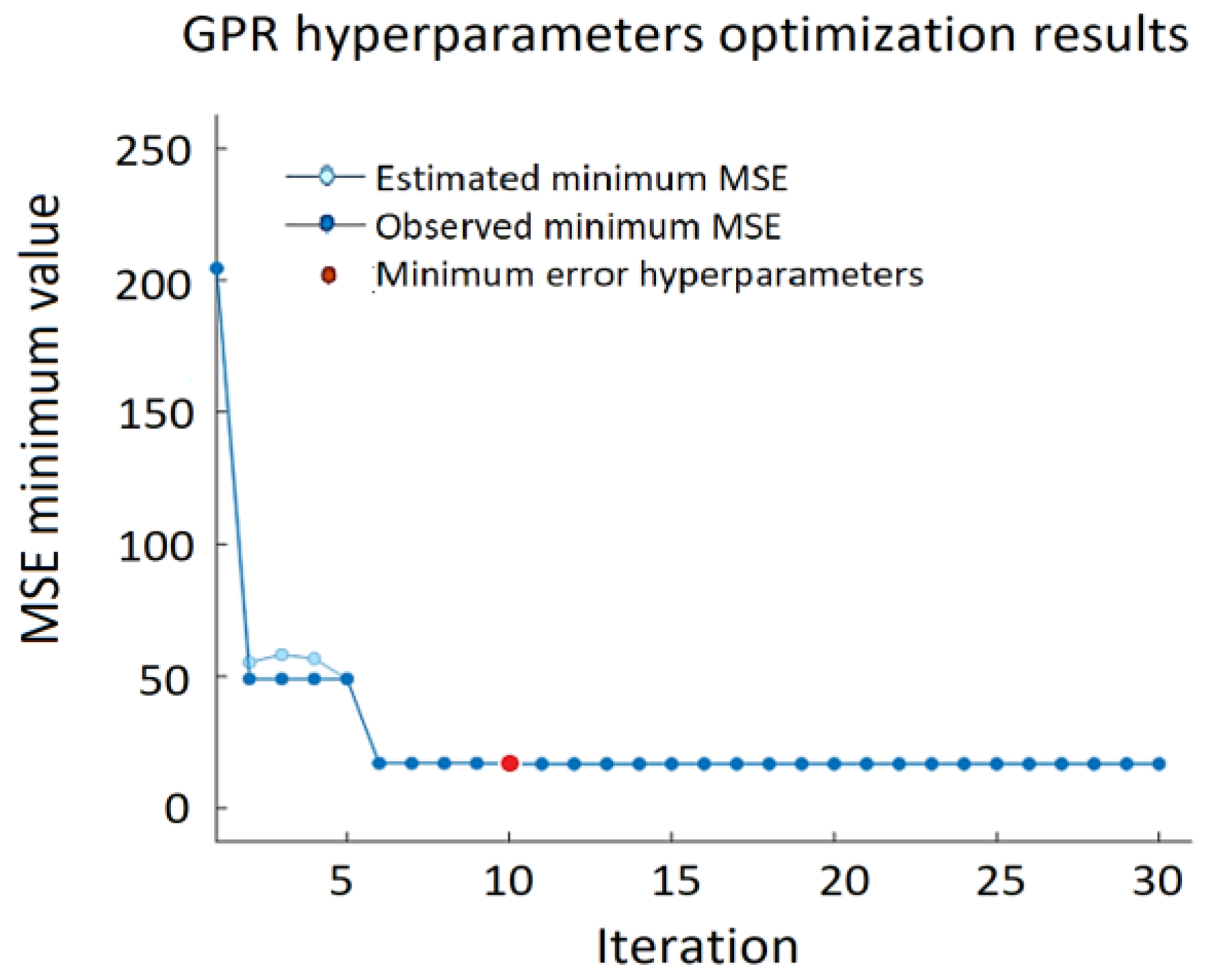
Figure 8 shows the minimum MSE of the GPR algorithm, where the red dot indicates the iteration with the minimum MSE, and the light blue dot represents the computed MSE value during the optimization process by varying the GPR hyperparameters. Dark blue dots indicate the observed minimum error minMSE detected up to the current (including current as well) observation:
where
n is the number of iterations.
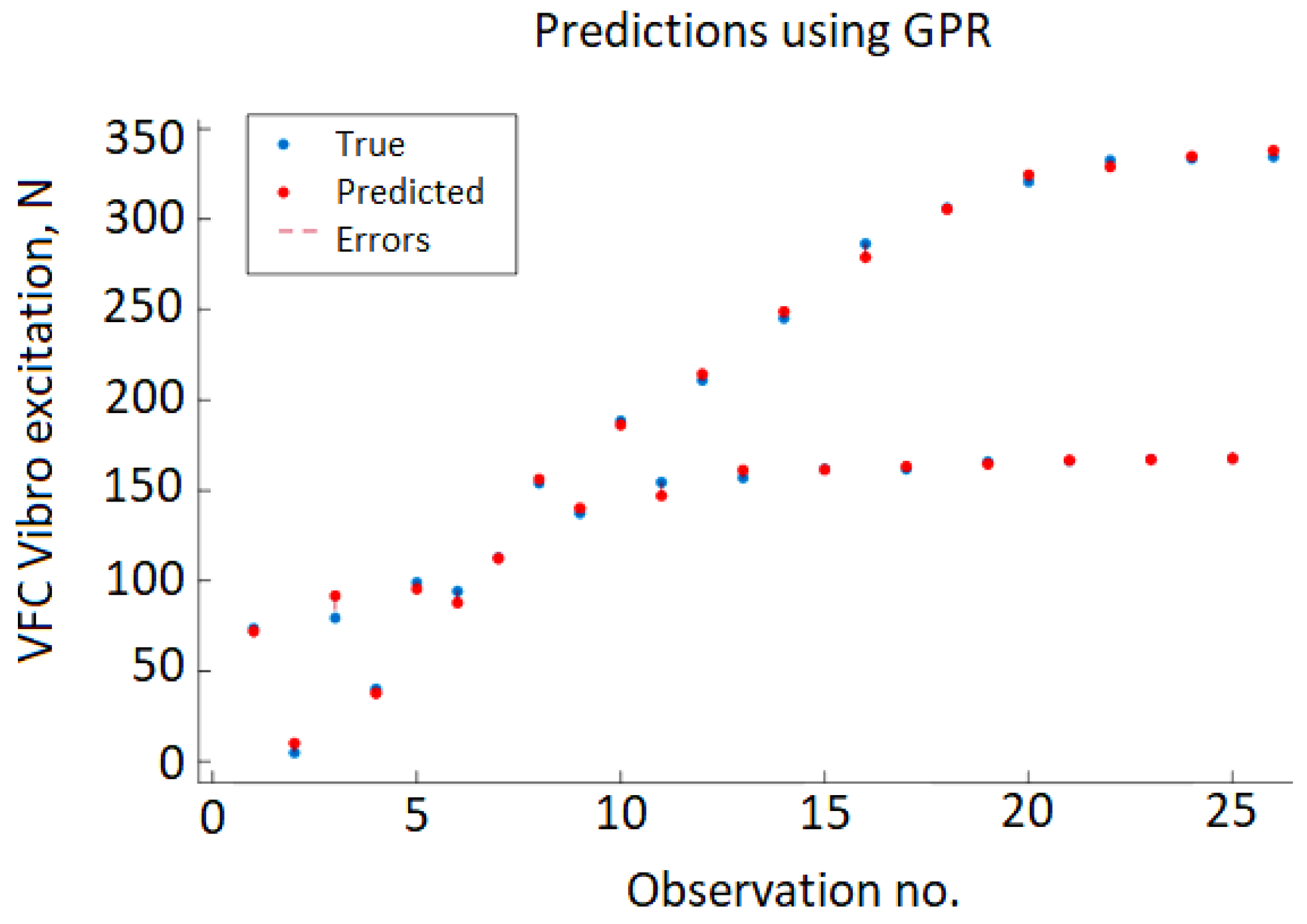
Figure 9 shows the cross-validation results depicting the predicted value of VFC vibro excitation against the real (true) values. The errors are represented by vertical red dashed lines, but due to very small error values, the majority of the true and predicted value points overlap.
The best results achieving
,
, and
have been achieved using a linear basic function, no-isotropic rational quadratic kernel function (Equation (8)) with sigma 0.0002.
where
—the overall variance,
—the length scale parameter,
—the scale-mixture (
.
Four hyperparameters have been included in the SVM model optimization process: kernel function, kernel scale, box constraint, and epsilon (
Table 8). The ranges of values for the latter three hyperparameters were selected on the basis of preliminary experiments. Seven different kernel functions have been analyzed: three Gaussian (fine, medium, coarse), Linear, Quadratic, and Cubic. It has been observed that the Gaussian functions gave the poorest results compared to other functions.
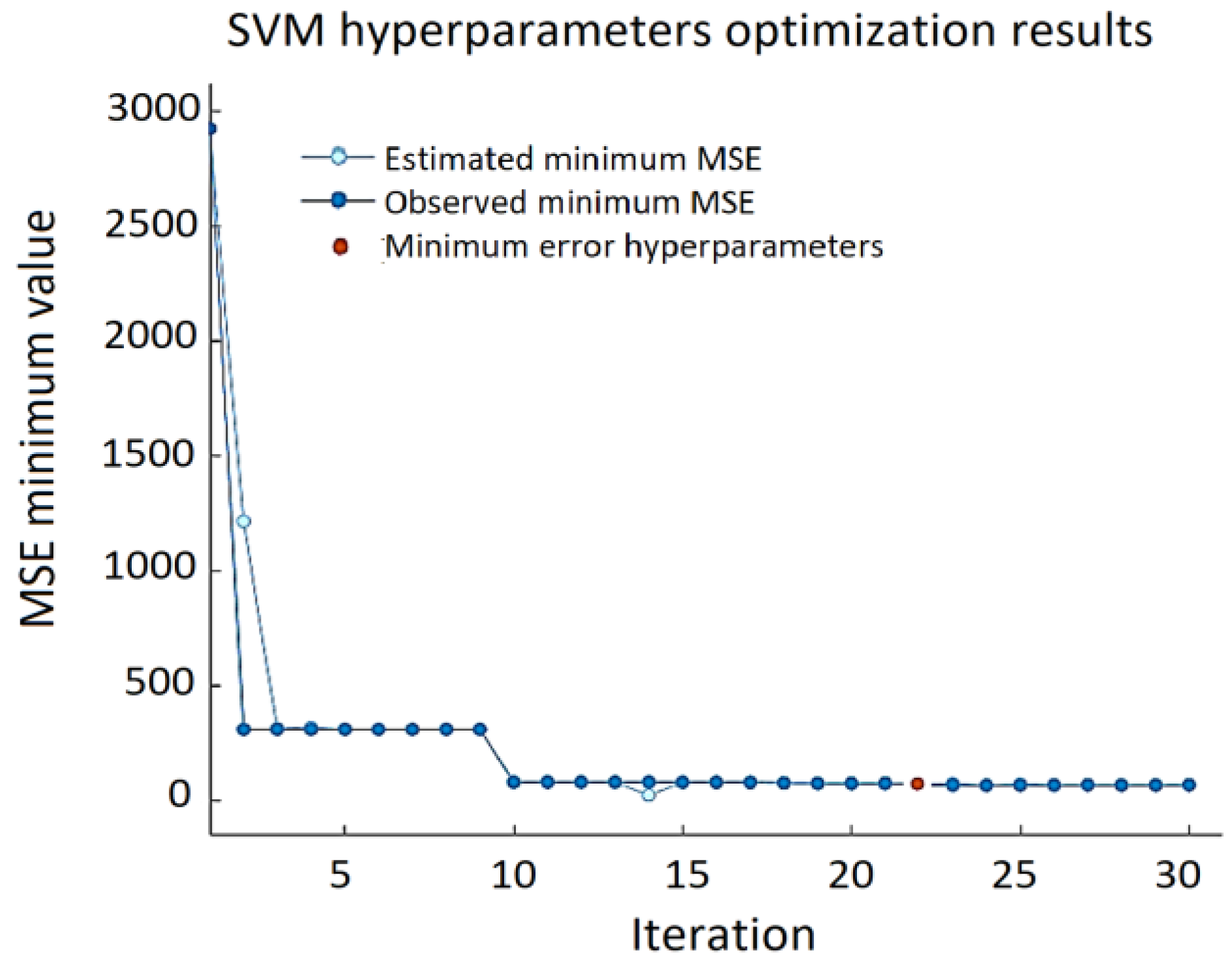
The best results for the validation set—RMSE = 9.124, MSE = 83.253, and MAE = 6.403—were obtained using a linear kernel function, ε = 0.105, with box constrains = 111.25 (
Figure 10).
It can be noted that the minimum MSE varies over a wide range depending on the combination of the SVM hyperparameters, and the error can reach almost 3000. Prediction errors are displayed in a response plot in
Figure 11.
For the ANN model experimental setup, we have used a simple feedforward network—multilayer perceptron (MLP), presented in
Figure 12.
As in the two previous ANN models, four hyperparameters were used in the optimization process: the number of hidden layers, the size of the hidden layer, the activation function of the hidden layers, and regularization strength (
Table 9). The three most common activation functions were analyzed: Sigmoid, Hyperbolic tangent (Tanh), and Rectified Linear Unit (ReLU). The range of regularization strength was chosen based on primary cross-validation results. Value ranges of hidden number layers and hidden layer size were selected according to the size of the data set.
The ANN approach provides very good prediction accuracy and the best results with RMSE = 4.5337, MSE = 20.573, and MAE = 3.528 were obtained using a single hidden layer neural network with ReLU activation function, 12 neurons, and a regularization strength of zero. The variation of the minimum MSE values during the ANN hypermeter optimization process is shown in
Figure 13. The testing data results of the ANN model are presented in
Figure 14 providing actual and predicted values of VFC vibration excitation.
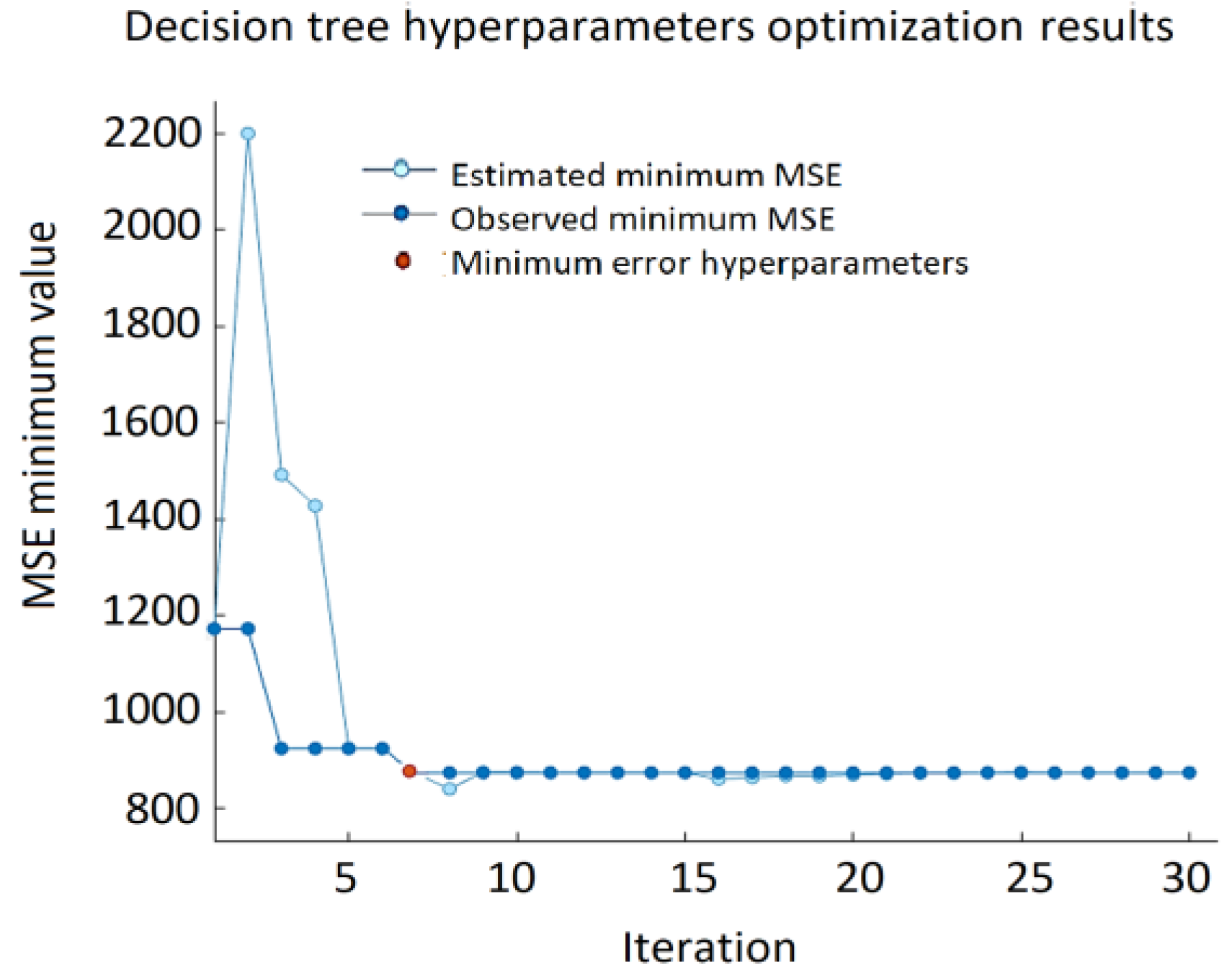
Thus, the minimum leaf size is the only hyperparameter that was included in the optimization. It denotes the minimum number of data points that are required to be present in the leaf node. The search range for this hyperparameter is from 1 to 15 which is chosen according to the size of the data set. The best result of the DT approach: RMSE = 29.567, MSE = 874.19, and MAE = 21.507 (
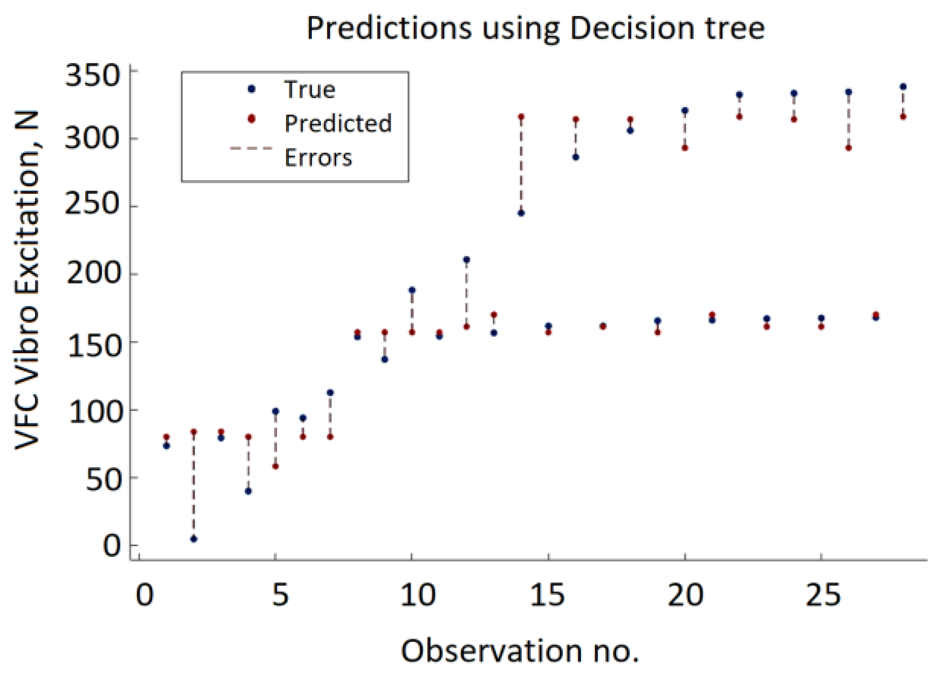
Figure 15) were obtained using a decision tree with a minimum leaf size equal to four. The decision tree approach provides the lowest accuracy compared to GPR, SVM, and ANN. The minimum MSE value varies from 2195.31 to 874.19. As depicted in
Figure 16, in half of the observations, the distance between the predicted VFC vibration excitation value and the actual values is more significant than GPR, ANN, or SVM.
Table 10 represents the hyperparameters of another, i.e., the KNN approach. Two KNN hyperparameters were included in the optimization process. The first one is K (the number of neighbors to consider) and the second is the employed distance function (most commonly used Euclidean, Manhattan, Minkowski).
For
n-dimensional space, the Euclidean distance between the two points
with coordinates
and
with coordinates
is determined using the following equation:
where
are attribute values of
y data instance and
are attribute values of
x data instance.
The Manhattan distance is also known as city block distance, or taxicab geometry, as well as several other names, because it allows calculating the distance between two data points on a uniform grid, for example, a city block; there may be more than one path between the two points that have the same Manhattan distance. The Manhattan distance between two points x and y is calculated using the formula:
Minkowski distance is a generalized distance metric. The above formula (Equation (10)) can be manipulated by substituting ‘
p’ to calculate the distance between two data points in different ways. Thus, Minkowski distance is also known as
Lp norm distance:
where
is the order of the Minkowski metric. With different values of
, the distance between two data points can be calculated in different ways:
—Manhattan distance;
—Euclidean distance,
—Chebyshev’s distance. A value such as
provides a balance between the two measures.
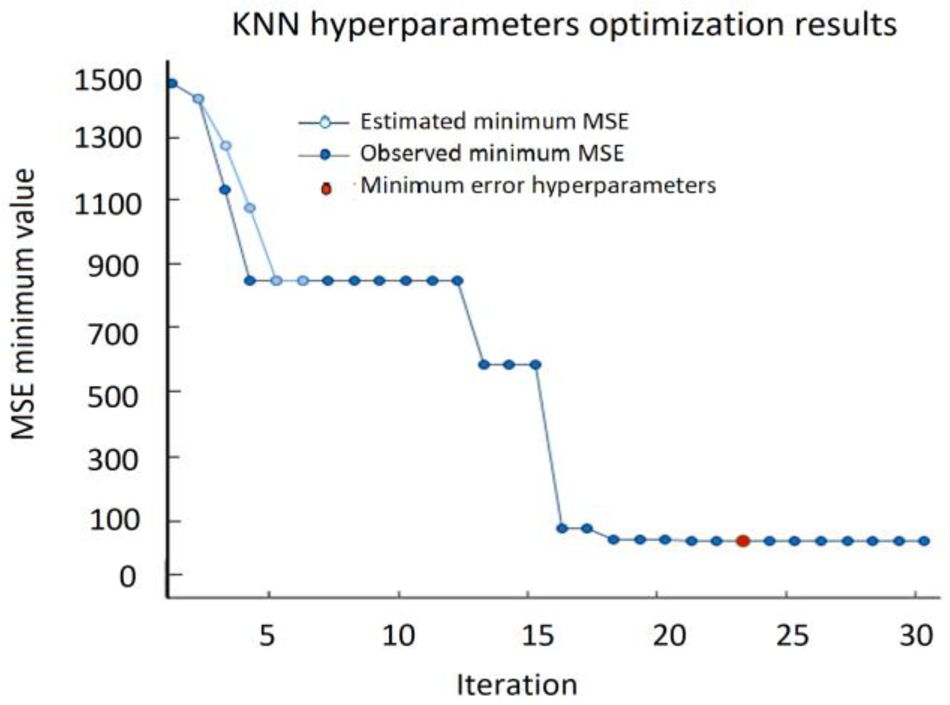
The best KNN results, including RMSE = 6.0757, MSE = 36.915, and MAE = 3.528 were obtained using the Manhattan distance for two neighbors,
K = 2 (
Figure 17).
The most important step in KNN is to determine the optimal value of
K. The optimal value of
K reduces the effect of noise on the classification. A technique called the “elbow method” helps to do this, selecting the optimal
K value. Different values of
K are applied to the same data set and the change in
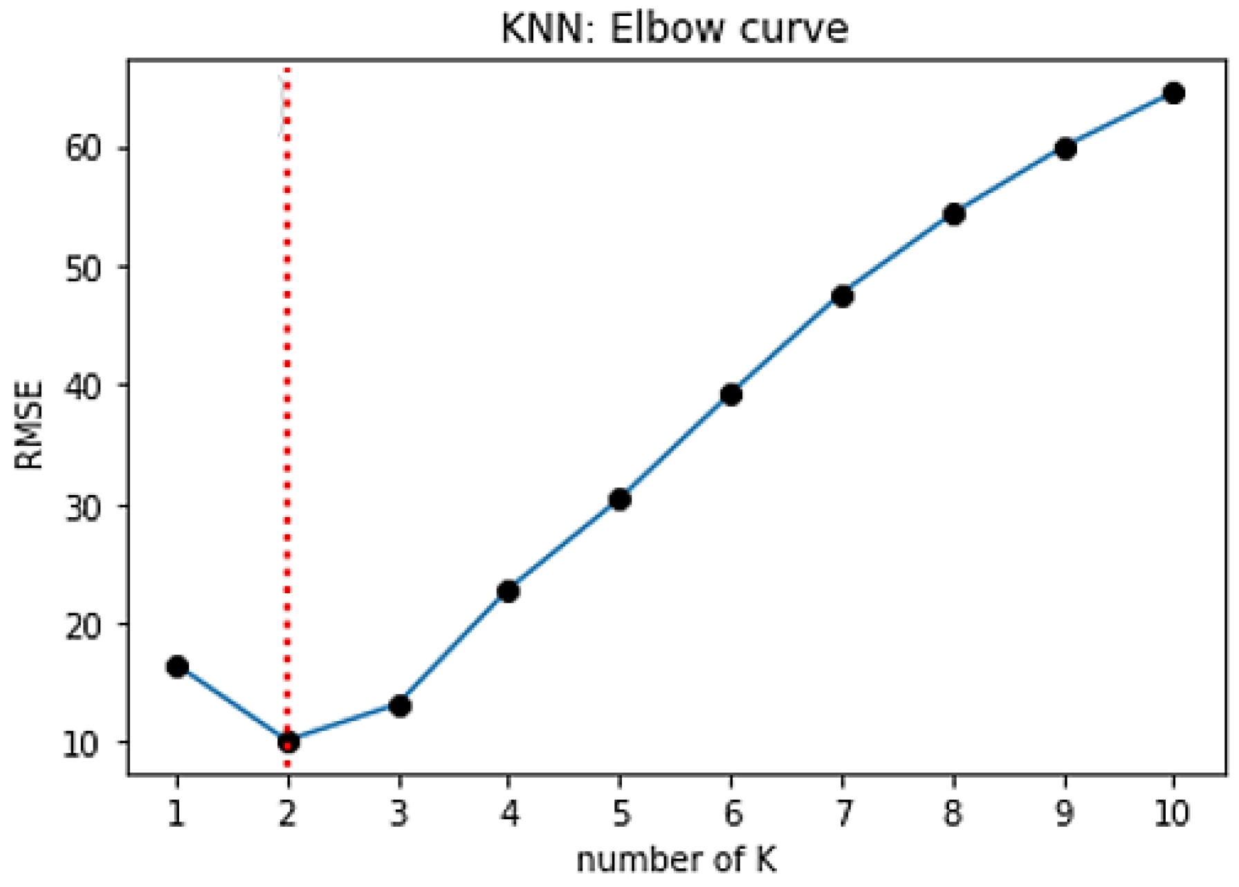
K is initially observed. In the data set characterizing the SPIF process, the error rate (RMSE) curve obtained by applying the KNN with respect to the
K value is shown in
Figure 18.
The graph presented in
Figure 18 denotes that initially the error rate decreases to 2, and then it starts to increase. Thus, the value of
K should be 2, i.e., it is the optimal
K value for this model. This curve is called an elbow curve because it has a shape of an elbow and is commonly used to adjust the
K value.
R2 (coefficient of determination) is a regression score, which is a statistical measure indicating how close the data are to the fitted regression line. In regression, it is a measure showing how well the regression predictions approximate the real data. An
R2 of 1 indicates that the regression predictions perfectly fit the data:
where
SSR is the sum of squares of residuals,
SST is the total sum of squares,
is the actual value,
is the predicted value, and
is the mean value.
R2 is always between 0 and 100% (or 0 and 1.0). The higher the
R2, the better the model. The goal is not to maximize
R2 because model stability and adaptability are equally important. When checking the adjusted
R2 value, it is preferred to have the values of the
R2 and adjusted
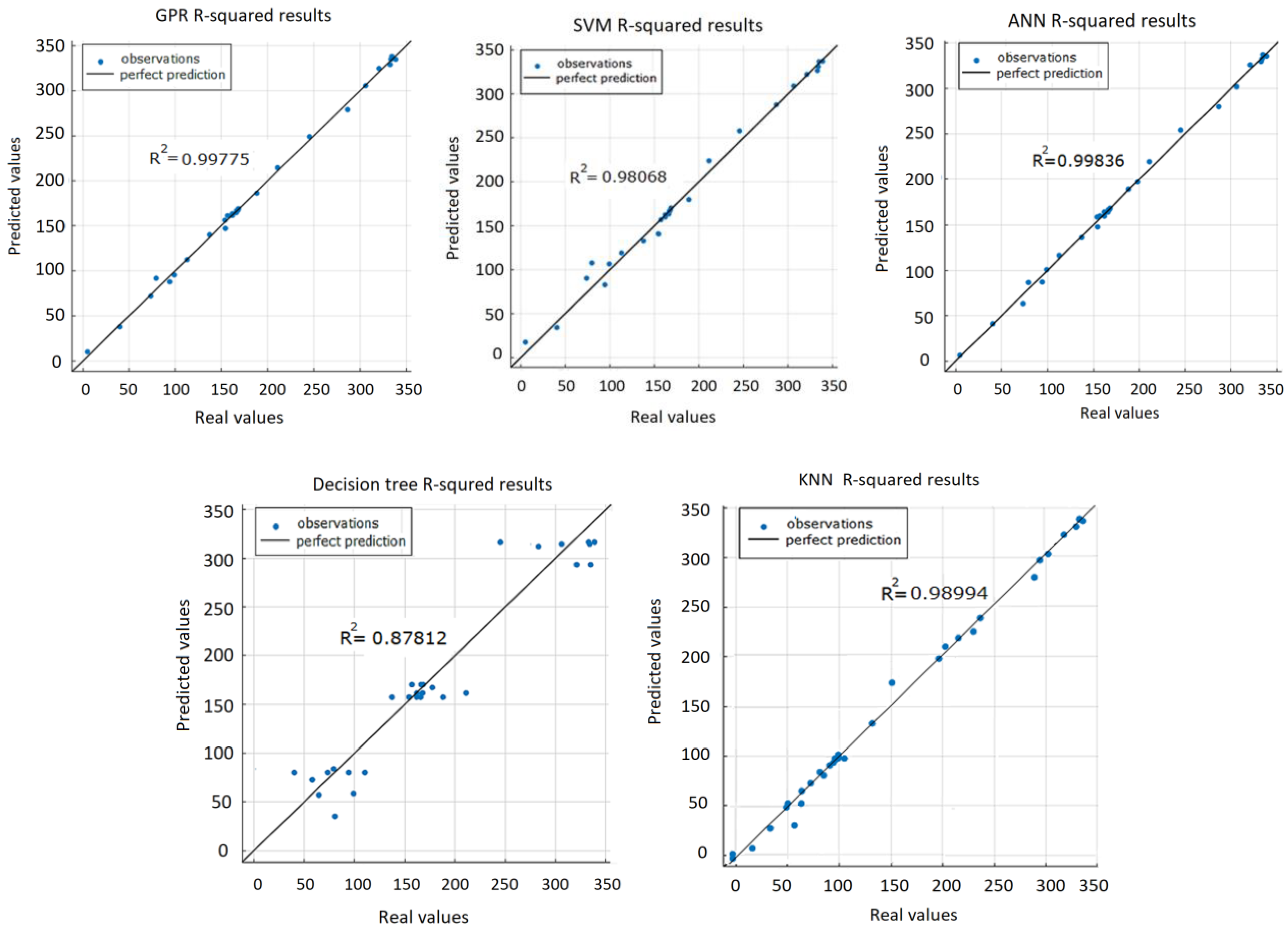
R2 close to each other. From the graphical representation of
R2 values of the five prediction models (
Figure 19), it can be seen that the DT algorithm gave the worst result (
R2 = 0.878) compared to others.
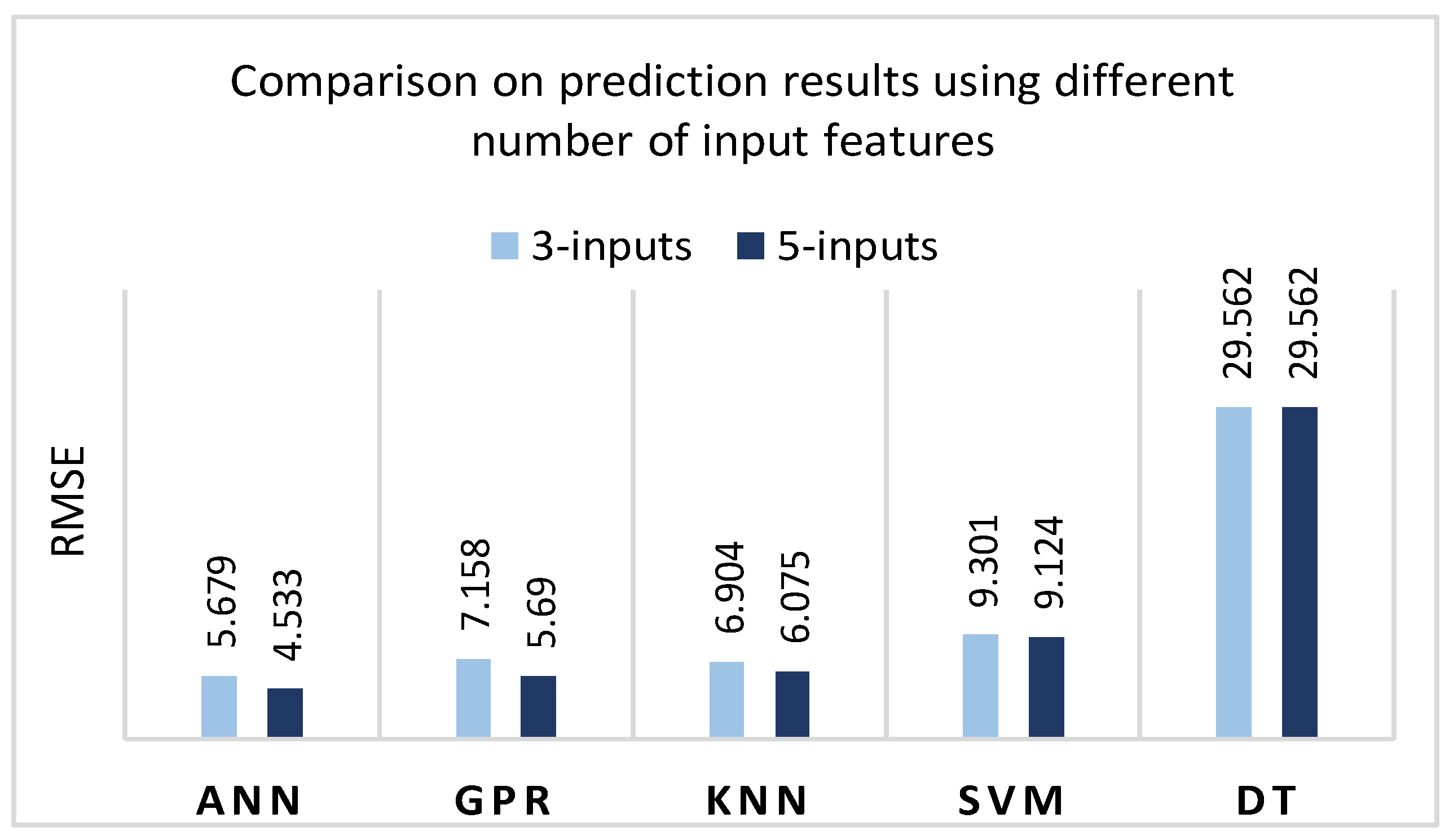
A series of five experimental runs have been carried. Summarizing the experimental results, ANN and GPR were identified as the most efficient methods for developing VFC vibro excitation prediction models, giving the lowest prediction error (RMSE) of 4.5337 and 5.6891, respectively (
Figure 20). It should be noted that the DT algorithm is inappropriate for this task and for the available data set, as the prediction errors in both cases (with and without optimization) are high, reaching around 30%. As for the standard deviation (ST), despite the DT model with a 0 value of ST for all five iterations, the GDR has the lowest standard deviation, ST = 0.201. The ANN model has resulted with ST = 0.616, KNN with ST = 0.78, and the SVM with the highest value, ST = 2.531.
