
Smart SDN Management of Fog Services to Optimize QoS and Energy

 ,
,  ,
,  , and
, and 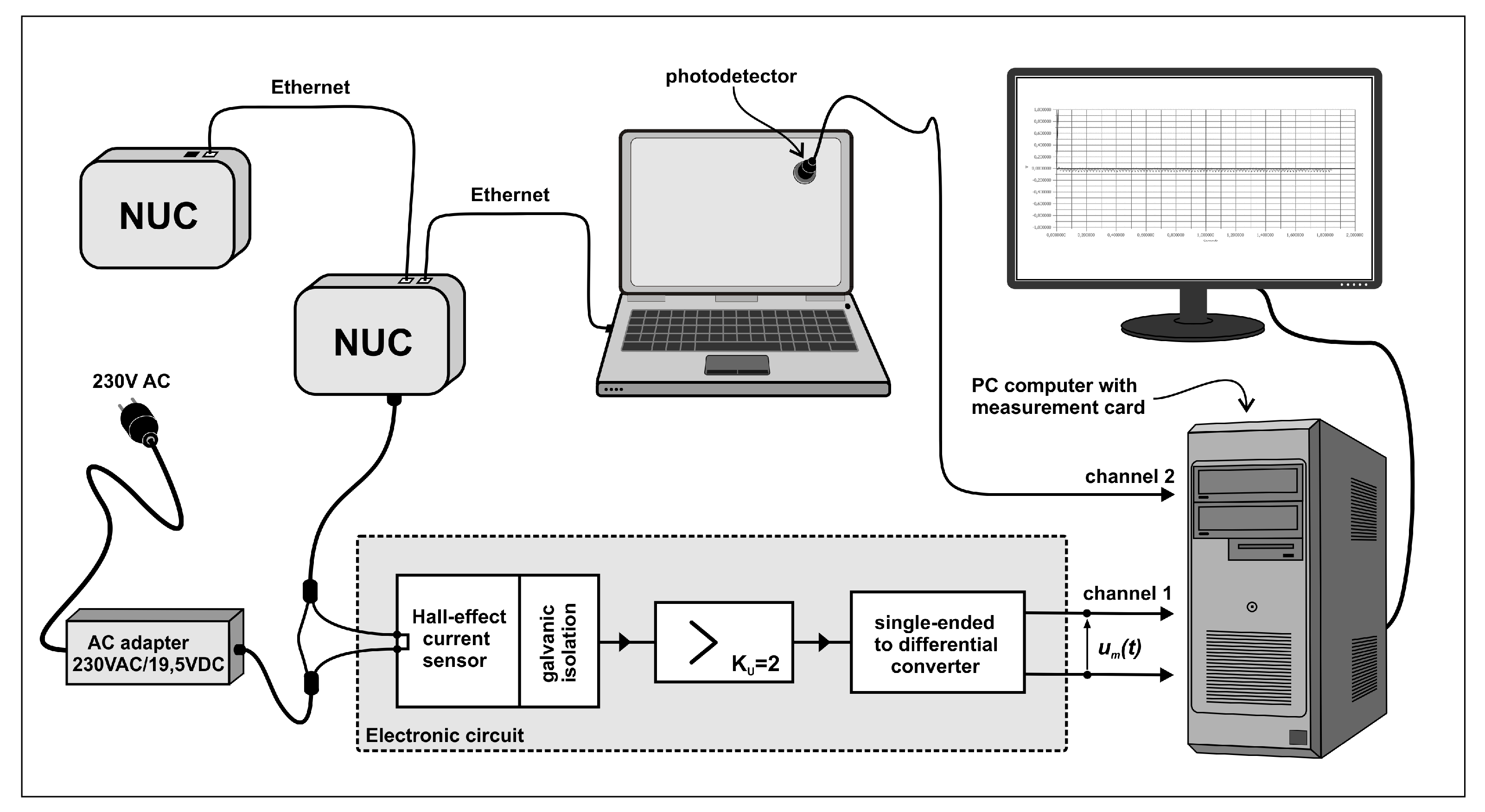
Abstract
1. Introduction
1.1. Optimization Techniques for SDN Networks and the Fog
1.2. Content of This Paper
- We constructed a new objective or “goal function” for client-to-service allocation, which combines the total response time experienced and measured at the client end (including the round-trip network delay and the service time at the server), plus the power consumed in the SDN network by the client request.
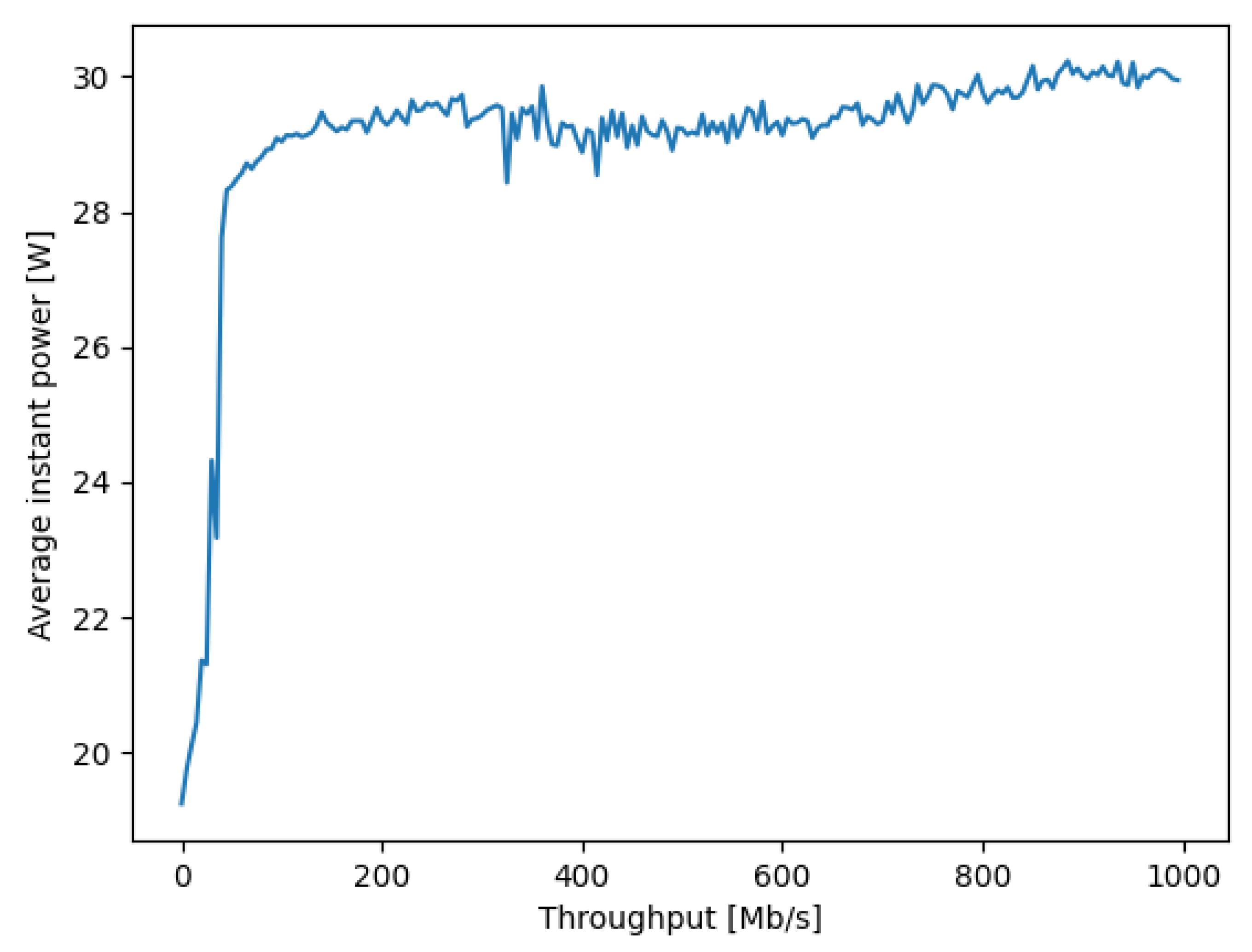
- Since load-dependent power measurements of the actual “NUC” hardware [45] that we use for each SDN switches is not available in the literature, we conducted accurate power versus traffic load measurements with a specific Hall effect apparatus. We note that the idle power consumption that we measured and report in Figure 1 is not negligible. Indeed while the NUC peak power consumption at maximum load is approximately 30 Watts, the idle consumption is approximately 20 Watts.
- We detailed the adaptive control algorithm based on RL [15] and a random neural network [46,47,48] that acts as an adaptic critic, using the real-time measurement of the overall service response time, including the round-trip delay to send the request and receive the result through the SDN network as well as the server response time for processing the service request, and the traffic-driven power consumption in the SDN network. Note that others have used the RNN as a tool for controlling the online performance of packet networks and mobile networks [49,50,51,52,53,54].
- This work extends on previous research that only addressed the network aspects with regard to QoS [41] and QoS and security [55]. We discuss in detail the computational complexity of the algorithm and show that it is where n is the number of different possible connection paths between clients and services.
- The RL algorithm is implemented in the SDN controller, and takes online decisions in real time that minimize the composite goal function.
- We show the effectiveness of our technique by exhibiting measurement results on a multi-hop SDN network, together with client software requests and servers, with multiple users and multiple servers. Our experiments show in particular that our adaptive controller achieves power savings of the order of 15% with a very moderate (but consistent) less than 2% increase in average response time.
2. The Decision System
- For each Fog node and client, we need to estimate the response time which is the overall time (including any waiting time) it takes the server f to service i for client u.
- Similarly, for the specific path , we will need to estimate the round-trip transfer time for transferring the service request and any needed data from u to the service i at f, and for transferring the results back from f to u.
- Finally, we will also require an estimate of the network power consumption for the request of client u for service i, which includes the round-trip transfer associated with the amount of data involved in the request, and the energy consumption characteristics of the SDN switches on the path .
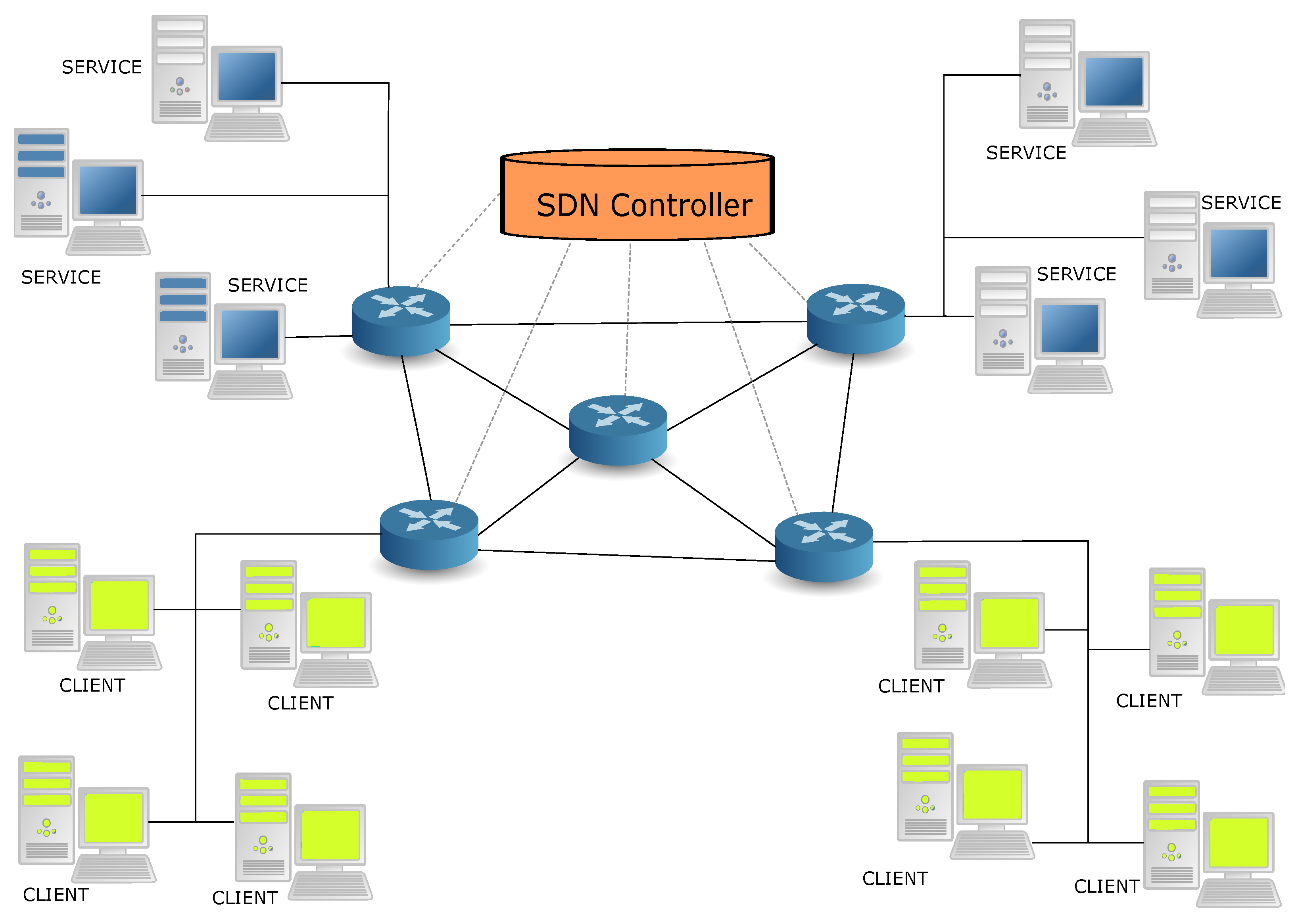
- Selecting the optimum path in the network to connect a user to a specific Fog server for a given service, since the choice of the path determines the choice of the Fog server that is selected.
- Moreover, the practical consequence is that this can be implemented by a SDN controller whose the normal function was to select a path in the network for a given connection.
2.1. Random Neural Network and Reinforcement Learning
The Reinforcement Learning Algorithm
- After server f is chosen to execute service i to satisfy the request of client u, the resulting total client response time, i.e., the first term in Equation , is measured from the simple difference of the time-stamp when the request is sent by the client and the time-stamp when the result is received by the client. The traffic rate on the path being used is also measured during the transfer of the request and the second term of is obtained from a table look-up of power consumption versus traffic rate. As a result, the value of the goal function is computed with two multiplications and one addition, from the measurement data regarding client response time and path consumption.
- The historical value of the “reward”, defined as the inverse of the goal, i.e., , defined as is updated:where is used to give more or less importance to the recent measurements. Note that this requires one division, two multiplications and one addition.
- Subsequently, the RNN weights are updated:
- Then, to prevent the weights from constantly increasing:
- Finally, with these updated values of the weights, we compute all the using the system of Equation (3), which is a fixed point iteration of complexity .
- Then, we obtain the new value of the best choice of path for the request from client u for service i, including the path itself and the Fog server at the end of the path:which uses comparison operations if we use Bubblesort, or if we use a more sophisticated sorting algorithm.
3. Linking Network Power Consumption to SDN Switch Traffic Rate
Measuring the Power Characteristic of the SDN Switches
4. The Test-Bed and the Experimental Results
4.1. Experimental Results Regarding the Response Time Only
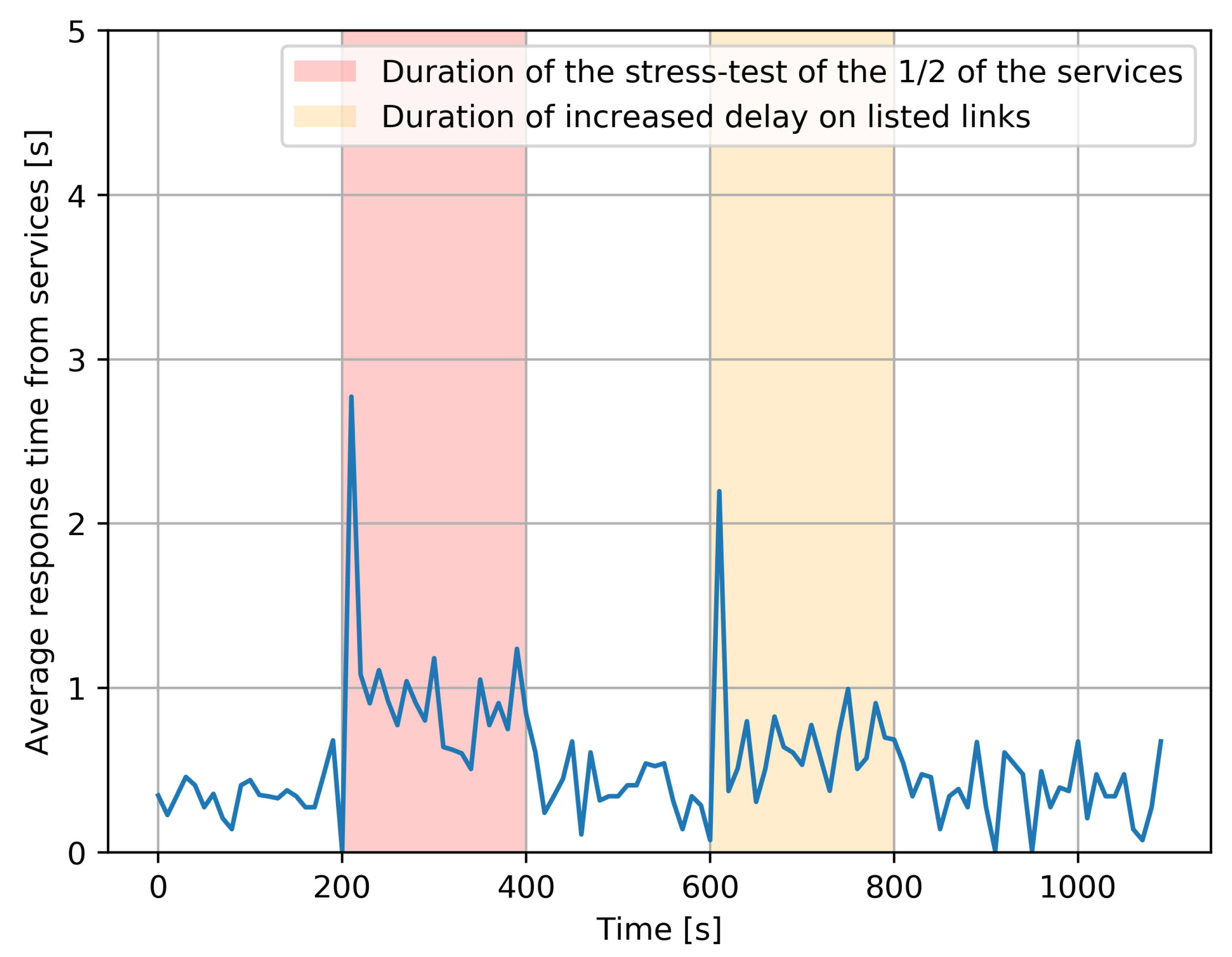
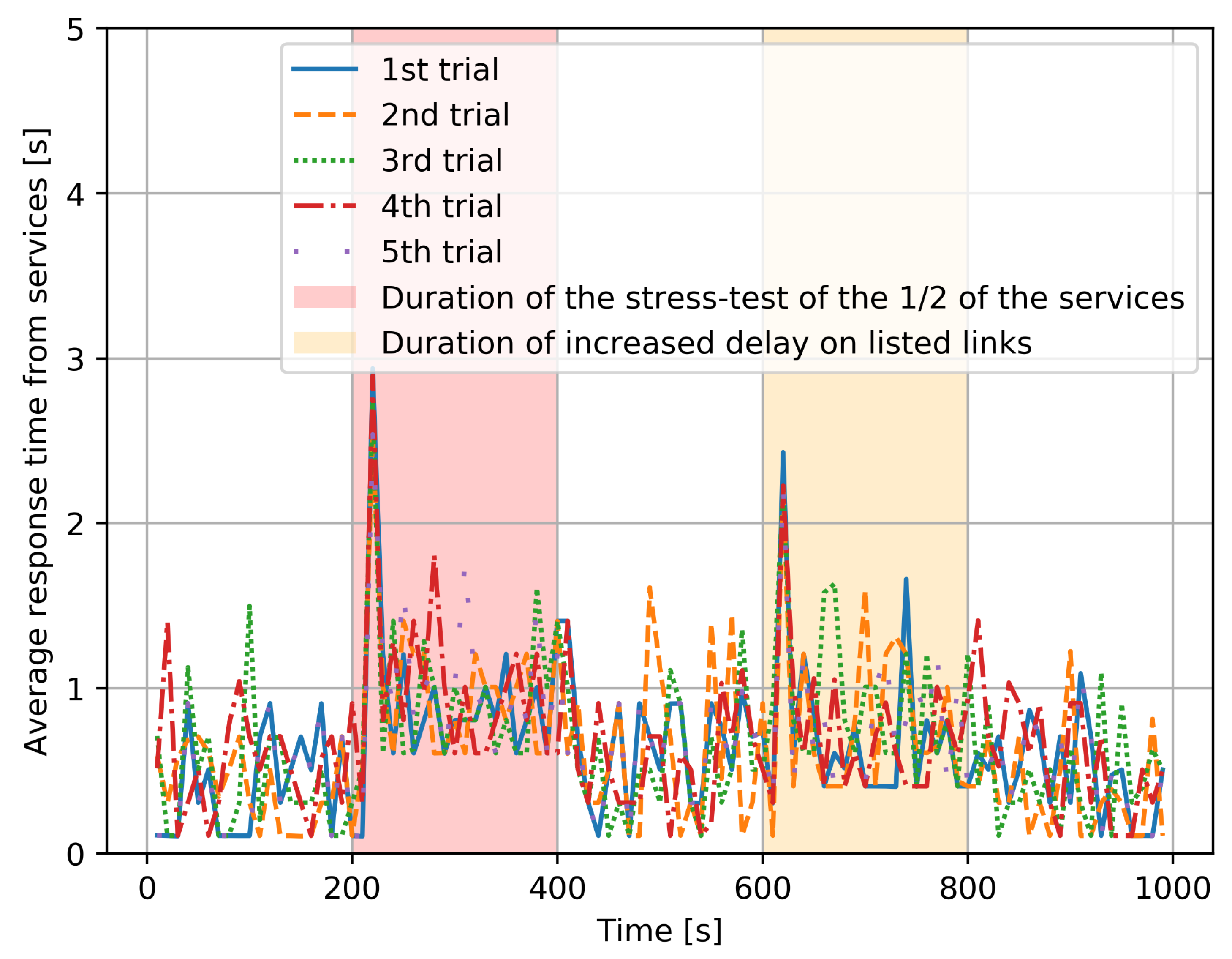
- In the time window , each client sent one request to one service, and all services are available and are responding as fast as they can. The resulting response time for the request which is satisfied for each user is denoted , from the instant when the user makes the request to the instant when the response is received back at the use. The overall average value of the n requests that are satisfied over the duration of the experiment is denoted:This experiment was repeated five times consecutively, and the overall average response time, which is an “average of averages”, taking the average of the 5 values of the individual average values T, is shown in Figure 5, in the part of the figure which does not have a background color.
- Secondly, the same experiment was run with a “stress test”, which is an additional program that executes 50% of the services which have been chosen at random, and simultaneously increases the CPU utilization rate to , resulting in a substantial increase in the time required to process the corresponding service requests. Its effect is shown with a red background in Figure 5. Interestingly, we notice that the effect of the stress test is mostly seen at the beginning of the “red period”, due to the RL-based adaptive control which dynamically shifts the load towards those service instances which do not have an overload. However, since 50% of services are systematically affected, we do have an increase in average response time. After the stress test ends, everything goes back to the prior condition.
- Thirdly, during the time span shown with an orange background in Figure 5, the links between , experience a major increase in delay caused by a DDoS attack. As a result, the clients also experience a major increase in response time due to the additional transfer delay of requests and of the corresponding responses. Again, we observe that the worse effect is at the beginning of the “yellow period”, since the RL-based adaptive control shifts the workload to the longer two-hop paths that are not under attack. Obviously, an increase in response time still occurs because of the longer paths, but it is not as bad as that at the beginning of the attack since the RL-based control has been able to avoid the links which are under attack. After the DDoS attack ends, the average response times fall back to “normal”.
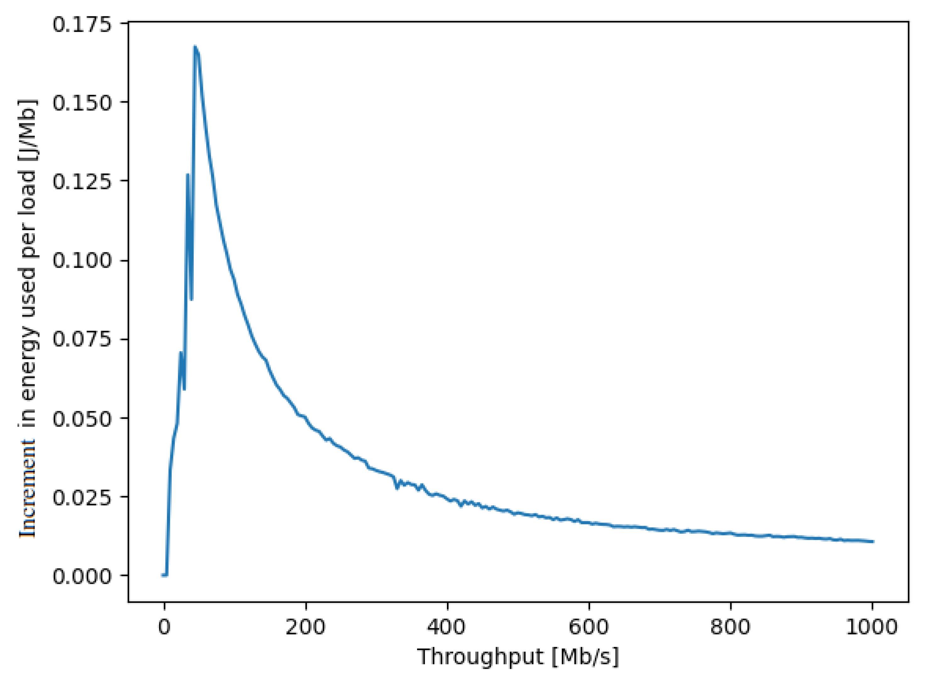
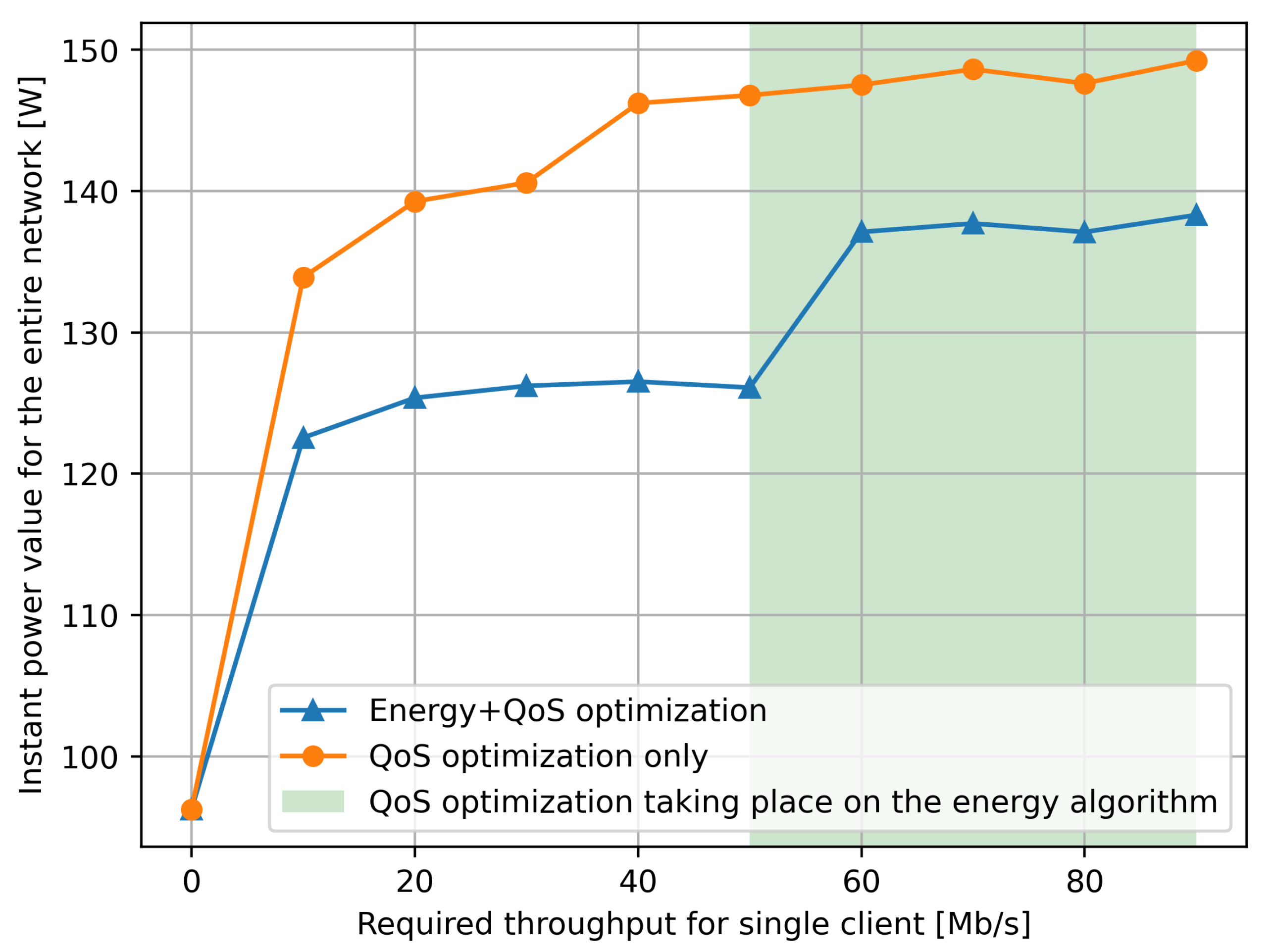
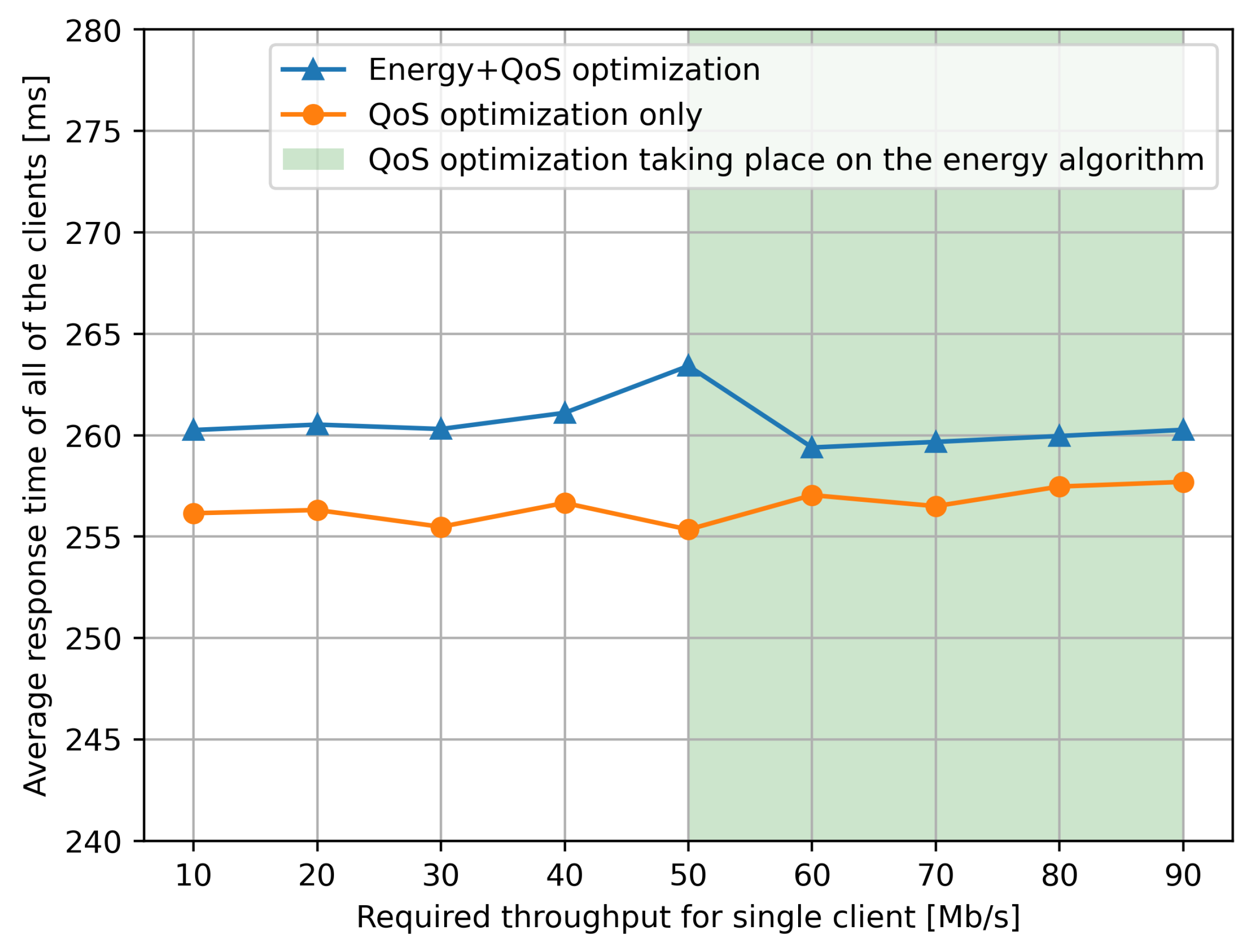
4.2. Experiments Concerning Energy Optimization
- Each client sends one request in the 10 s time window as described in the previous section.
- The actual throughput is measured at the SDN switches (NUCs) and the instantaneous power consumption is computed from Figure 2.
5. Conclusions
Author Contributions
Funding
Institutional Review Board Statement
Informed Consent Statement
Conflicts of Interest
References
- Buyya, R.; Srirama, S.N.; Casale, G.; Calheiros, R.; Simmhan, Y.; Varghese, B.; Gelenbe, E.; Javadi, B.; Vaquero, L.M.; Netto, M.A.S.; et al. A Manifesto for Future Generation Cloud Computing: Research Directions for the Next Decade. ACM Comput. Surv. 2019, 51, 105:1–105:38. [Google Scholar] [CrossRef]
- Levin, A.; Barabash, K.; Ben-Itzhak, S.G.; Schour, L. Networking Architecture for Seamless Cloud Interoperability. In Proceedings of the 2015 IEEE 8th International Conference on Cloud Computing, New York, NY, USA, 27 June–2 July 2015; pp. 1021–1024. [Google Scholar] [CrossRef]
- Bonomi, F.; Milito, R.; Zhu, J.; Addepalli, S. Fog computing and its role in the internet of things. In Proceedings of the First Edition of the MCC Workshop on Mobile Cloud Computing, Helsinki, Finland, 17 August 2012; pp. 13–16. [Google Scholar] [CrossRef]
- Mahmud, R.; Srirama, S.N.; Ramamohanarao, K.; Buyya, R. Profit-aware application placement for integrated Fog-Cloud computing environments. J. Parallel Distrib. Comput. 2020, 135, 177–190. [Google Scholar] [CrossRef]
- Radoslav, C. Cloud Computing Statistics 2019. Available online: https://techjury.net/blog/cloud-computing-statistics/#gref (accessed on 23 March 2021).
- Goasduff, L. Gartner Says 5.8 Billion Enterprise and Automotive IoT Endpoints Will Be in Use in 2020. Available online: https://www.gartner.com/en/newsroom/press-releases/2019-08-29-gartner-says-5-8-billion-enterprise-and-automotive-io (accessed on 23 March 2021).
- Gelenbe, E.; Sevcik, K.C. Analysis of Update Synchronization for Multiple Copy Data Bases. IEEE Trans. Comput. 1979, 28, 737–747. [Google Scholar] [CrossRef]
- Kim, C.; Kameda, H. An algorithm for optimal static load balancing in distributed computer systems. IEEE Trans. Comput. 1992, 41, 381–384. [Google Scholar]
- Topcuoglu, H.; Hariri, S.; Wu, M.Y. Performance-effective and low-complexity task scheduling for the Bera erogeneous computing. IEEE Trans. Parallel Distrib. Syst. 2002, 13, 260–274. [Google Scholar] [CrossRef]
- Zhu, X.; Qin, X.; Qiu, M. Qos-aware fault-tolerant scheduling for real-time tasks on heterogeneous clusters. IEEE Trans. Comput. 2011, 60, 800–812. [Google Scholar]
- Tian, W.; Zhao, Y.; Zhong, Y.; Xu, M.; Jing, C. A dynamic and integrated load-balancing scheduling algorithm for cloud datacenters. In Proceedings of the 2011 IEEE International Conference on Cloud Computing and Intelligence Systems, Beijing, China, 15–17 September 2011; pp. 311–315. [Google Scholar]
- Zhang, Z.; Zhang, X. A load balancing mechanism based on ant colony and complex network theory in open cloud computing federation. In Proceedings of the 2010 The 2nd International Conference on Industrial Mechatronics and Automation, Wuhan, China, 30–31 May 2010; Volume 2, pp. 240–243. [Google Scholar]
- Dobson, S.; Denazis, S.; Fernández, A.; Gaïti, D.; Gelenbe, E.; Massacci, F.; Nixon, P.; Saffre, F.; Schmidt, N.; Zambonelli, F. A survey of autonomic communications. ACM Trans. Auton. Adapt. Syst. 2006, 1, 223–259. [Google Scholar] [CrossRef]
- Wang, L.; Brun, O.; Gelenbe, E. Adaptive workload distribution for local and remote Clouds. In Proceedings of the 2016 IEEE International Conference on Systems, Man, and Cybernetics (SMC), Budapest, Hungary, 9–12 October 2016; pp. 3984–3988. [Google Scholar]
- Sutton, R.S.; Barto, A.G. Reinforcement Learning: An Introduction, 2nd ed.; MIT Press: Cambridge, MA, USA, 2018. [Google Scholar]
- Yin, Y. Deep Learning with the Random Neural Network and its Applications. arXiv 2018, arXiv:1810.08653. [Google Scholar]
- François, F.; Gelenbe, E. Towards a cognitive routing engine for software defined networks. In Proceedings of the 2016 IEEE International Conference on Communications (ICC), Kuala Lumpur, 22–27 May 2016; pp. 1–6. [Google Scholar] [CrossRef]
- Xu, C.; Zhuang, W.; Zhang, H. A Deep-Reinforcement Learning Approach for SDN Routing Optimization. In Proceedings of the 4th International Conference on Computer Science and Application Engineering, CSAE 2020, Sanya, China, 19–21 October 2020. [Google Scholar] [CrossRef]
- Pernici, B.; Aiello, M.; Vom Brocke, J.; Donnellan, B.; Gelenbe, E.; Kretsis, M. What IS can do for environmental sustainability: A report from CAiSE’11 panel on Green and sustainable IS. Commun. Assoc. Inf. Syst. 2012, 30, 18. [Google Scholar] [CrossRef][Green Version]
- Çaglayan, M.U. Some Current Cybersecurity Research in Europe. In Security in Computer and Information Sciences, Proceedings of the First International ISCIS Security Workshop 2018, Euro-CYBERSEC 2018, London, UK, 26–27 February 2018; Revised Selected Papers, Communications in Computer and Information Science; Springer: Berlin/Heidelberg, Germany, 2018; Volume 821, pp. 1–10. [Google Scholar] [CrossRef]
- Aytaç, S.; Ermis, O.; Çaglayan, M.U.; Alagöz, F. Authenticated Quality of Service Aware Routing in Software Defined Networks. In Risks and Security of Internet and Systems, Proceedings of the 13th International Conference, CRiSIS 2018, Arcachon, France, 16–18 October 2018; Revised Selected Papers, Lecture Notes in Computer Science; Springer: Berlin/Heidelberg, Germany, 2018; Volume 11391, pp. 110–127. [Google Scholar] [CrossRef]
- Çaglayan, M.U. Performance, Energy Savings and Security: An Introduction. In Modelling, Analysis, and Simulation of Computer and Telecommunication Systems, Proceedings of the 28th International Symposium, MASCOTS 2020; Revised Selected Papers, Lecture Notes in Computer Science; Springer: Berlin/Heidelberg, Germany, 2021; Volume 12527, pp. 3–28. [Google Scholar] [CrossRef]
- Bera, S.; Misra, S.; Vasilakos, A.V. Software-defined networking for Internet of Things: A survey. IEEE Internet Things J. 2017, 4, 1994–2008. [Google Scholar] [CrossRef]
- Mambretti, J.; Chen, J.; Yeh, F. Next Generation Clouds, the Chameleon Cloud Testbed, and Software Defined Networking (SDN). In Proceedings of the 2015 International Conference on Cloud Computing Research and Innovation (ICCCRI), Singapore, 26–27 October 2015; pp. 73–79. [Google Scholar] [CrossRef]
- OpenFlow Switch Specification. 2015. Available online: https://opennetworking.org/wp-content/uploads/2014/10/openflow-switch-v1.5.1.pdf (accessed on 23 March 2021).
- Mouradian, C.; Naboulsi, D.; Yangui, S.; Glitho, R.H.; Morrow, M.J.; Polakos, P.A. A Comprehensive Survey on Fog Computing: State-of-the-Art and Research Challenges. IEEE Commun. Surv. Tutor. 2018, 20, 416–464. [Google Scholar] [CrossRef]
- Kehagias, D.; Jankovic, M.; Siavvas, M.; Gelenbe, E. Investigating the Interaction between Energy Consumption, Quality of Service, Reliability, Security, and Maintainability of Computer Systems and Networks. SN Comput. Sci. 2021, 2, 1–6. [Google Scholar]
- Rawat, D.B.; Lenkala, S.R. Software Defined Networking Architecture, Security and Energy Efficiency: A Survey. IEEE Commun. Surv. Tutor. 2017, 19, 325–346. [Google Scholar] [CrossRef]
- Huang, X.; Cheng, S.; Cao, K.; Cong, P.; Wei, T.; Hu, S. A Survey of Deployment Solutions and Optimization Strategies for Hybrid SDN Networks. IEEE Commun. Surv. Tutor. 2019, 21, 1483–1507. [Google Scholar] [CrossRef]
- Tajiki, M.M.; Akbari, B.; Shojafar, M.; Mokari, N. Joint QoS and Congestion Control Based on Traffic Prediction in SDN. Appl. Sci. 2017, 7, 1265. [Google Scholar] [CrossRef]
- Tajiki, M.M.; Shojafar, M.; Akbari, B.; Salsano, S.; Conti, M.; Singhal, M. Joint failure recovery, fault prevention, and energy-efficient resource management for real-time SFC in fog-supported SDN. Comput. Netw. 2019, 162, 6. [Google Scholar] [CrossRef]
- Ozdaglar, A.; Menache, I. Network Games: Theory, Models, and Dynamics; Morgan and Claypool: Williston, VT, USA, 2011. [Google Scholar] [CrossRef]
- Gelenbe, E. Analysis of single and networked auctions. ACM Trans. Internet Technol. 2009, 9, 8:1–8:24. [Google Scholar] [CrossRef]
- Du, J.; Gelenbe, E.; Jiang, C.; Zhang, H.; Ren, Y. Contract design for traffic offloading and resource allocation in heterogeneous ultra-dense networks. IEEE J. Sel. Areas Commun. 2017, 35, 2457–2467. [Google Scholar] [CrossRef]
- Gelenbe, E.; Lent, R. Energy-QoS Trade-Offs in Mobile Service Selection. Future Internet 2013, 5, 128–139. [Google Scholar] [CrossRef]
- Gelenbe, E.; Lent, R.; Douratsos, M. Choosing a Local or Remote Cloud. In Proceedings of the Second Symposium on Network Cloud Computing and Applications, NCCA 2012, London, UK, 3–4 December 2012; pp. 25–30. [Google Scholar] [CrossRef]
- Gelenbe, E.; Mitrani, I. Analysis and Synthesis of Computer Systems; World Scientific: Singapore, 2010; Volume 4. [Google Scholar]
- Foley, R.; McDonald, D. Join the shortest queue: Stability and exact asymptotics. Ann. Appl. Probab. 2001, 11, 569–607. [Google Scholar] [CrossRef]
- Fayolle, G. Functional Equations as an Important Analytic Method in Stochastic Modelling and in Combinatorics. Markov Process. Relat. Fields 2018, 24, 811–846. [Google Scholar]
- Paris, S.; Paschos, G.S.; Leguay, J. Dynamic control for failure recovery and flow reconfiguration in SDN. In Proceedings of the 2016 12th International Conference on the Design of Reliable Communication Networks (DRCN), Paris, France, 15–17 March 2016; pp. 152–159. [Google Scholar] [CrossRef]
- Gelenbe, E. Steps toward self-aware networks. Commun. ACM 2009, 52, 66–75. [Google Scholar] [CrossRef]
- Brun, O.; Wang, L.; Gelenbe, E. Big data for autonomic intercontinental overlays. IEEE J. Sel. Areas Commun. 2016, 34, 575–583. [Google Scholar] [CrossRef]
- Majdoub, M.; Kamel, A.E.; Youssef, H. Routing Optimization in SDN using Scalable Load Prediction. In Proceedings of the 2019 Global Information Infrastructure and Networking Symposium (GIIS), Paris, France, 18–20 December 2019; pp. 1–6. [Google Scholar] [CrossRef]
- Fröhlich, P.; Gelenbe, E.; Nowak, M.P. Smart SDN Management of Fog Services. In Proceedings of the 2020 Global Internet of Things Summit (GIoTS), Dublin, Ireland, 3 June 2020; pp. 1–6. [Google Scholar] [CrossRef]
- Intel. NUC—Small Form Factor Mini PC. 2021. Available online: https://en.wikipedia.org/wiki/Next-Unit-of-Computing (accessed on 23 March 2021).
- Gelenbe, E. Random neural networks with negative and positive signals and product form solution. Neural Comput. 1989, 1, 502–510. [Google Scholar] [CrossRef]
- Sakellari, G. The cognitive packet network: A survey. Comput. J. 2010, 53, 268–279. [Google Scholar] [CrossRef]
- Basterrech, S.; Rubino, G. A Tutorial about Random Neural Networks in Supervised Learning. Neural Netw. World 2016, 25, 457–499. [Google Scholar] [CrossRef]
- Mohamed, S.; Rubino, G.; Varela, M. Performance evaluation of real-time speech through a packet network: A random neural networks-based approach. Perform. Eval. 2004, 57, 141–161. [Google Scholar] [CrossRef]
- Cramer, C.E.; Gelenbe, E. Video quality and traffic QoS in learning-based subsampled and receiver-interpolated video sequences. IEEE J. Sel. Areas Commun. 2000, 18, 150–167. [Google Scholar] [CrossRef]
- Sakellari, G. Performance evaluation of the Cognitive Packet Network in the presence of network worms. Perform. Eval. 2011, 68, 927–937. [Google Scholar] [CrossRef]
- Adeel, A.; Larijani, H.; Ahmadinia, A. Resource Management and Inter-Cell-Interference Coordination in LTE Uplink System Using Random Neural Network and Optimization. IEEE Access 2015, 3, 1963–1979. [Google Scholar] [CrossRef]
- Adeel, A.; Larijani, H.; Ahmadinia, A. Random neural network based novel decision making framework for optimized and autonomous power control in LTE uplink system. Phys. Commun. 2016, 19, 106–117. [Google Scholar] [CrossRef]
- Adeel, A.; Larijani, H.; Ahmadinia, A. Random neural network based cognitive engines for adaptive modulation and coding in LTE downlink systems. Comput. Electr. Eng. 2017, 57, 336–350. [Google Scholar] [CrossRef]
- Gelenbe, E.; Domanska, J.; Fröhlich, P.; Nowak, M.P.; Nowak, S. Self-Aware Networks that Optimize Security, QoS, and Energy. Proc. IEEE 2020, 108, 1150–1167. [Google Scholar] [CrossRef]
- Gelenbe, E.; Stafylopatis, A. Global behavior of homogeneous random neural systems. Appl. Math. Model. 1991, 15, 534–541. [Google Scholar] [CrossRef]
- ONOS. Home Page of ONOS Project—Open Source SDN Controller. 2021. Available online: https://onosproject.org (accessed on 23 March 2021).


Publisher’s Note: MDPI stays neutral with regard to jurisdictional claims in published maps and institutional affiliations. |
© 2021 by the authors. Licensee MDPI, Basel, Switzerland. This article is an open access article distributed under the terms and conditions of the Creative Commons Attribution (CC BY) license (https://creativecommons.org/licenses/by/4.0/).
Share and Cite
Fröhlich, P.; Gelenbe, E.; Fiołka, J.; Chęciński, J.; Nowak, M.; Filus, Z. Smart SDN Management of Fog Services to Optimize QoS and Energy. Sensors 2021, 21, 3105. https://doi.org/10.3390/s21093105
Fröhlich P, Gelenbe E, Fiołka J, Chęciński J, Nowak M, Filus Z. Smart SDN Management of Fog Services to Optimize QoS and Energy. Sensors. 2021; 21(9):3105. https://doi.org/10.3390/s21093105
Chicago/Turabian StyleFröhlich, Piotr, Erol Gelenbe, Jerzy Fiołka, Jacek Chęciński, Mateusz Nowak, and Zdzisław Filus. 2021. "Smart SDN Management of Fog Services to Optimize QoS and Energy" Sensors 21, no. 9: 3105. https://doi.org/10.3390/s21093105
APA StyleFröhlich, P., Gelenbe, E., Fiołka, J., Chęciński, J., Nowak, M., & Filus, Z. (2021). Smart SDN Management of Fog Services to Optimize QoS and Energy. Sensors, 21(9), 3105. https://doi.org/10.3390/s21093105