
Multi-Dimension and Multi-Feature Hybrid Learning Network for Classifying the Sub Pathological Type of Lung Nodules through LDCT

Abstract
1. Introduction
2. Materials and Methods
2.1. Dataset
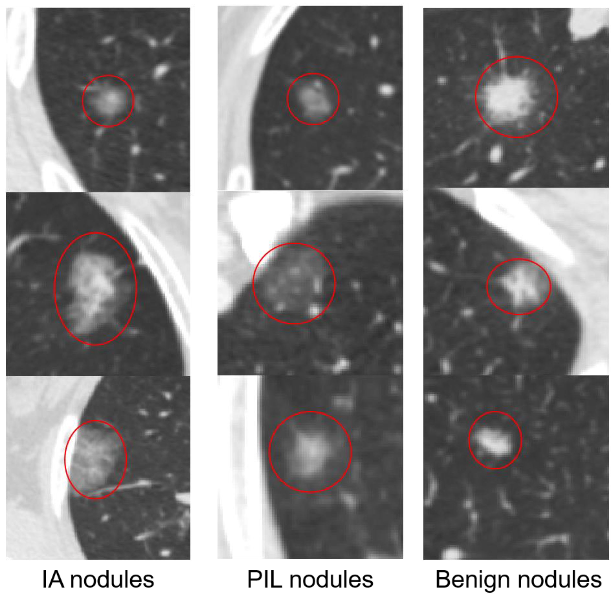
2.1.1. 2D Samples
2.1.2. 3D Samples
2.2. Network Architecture
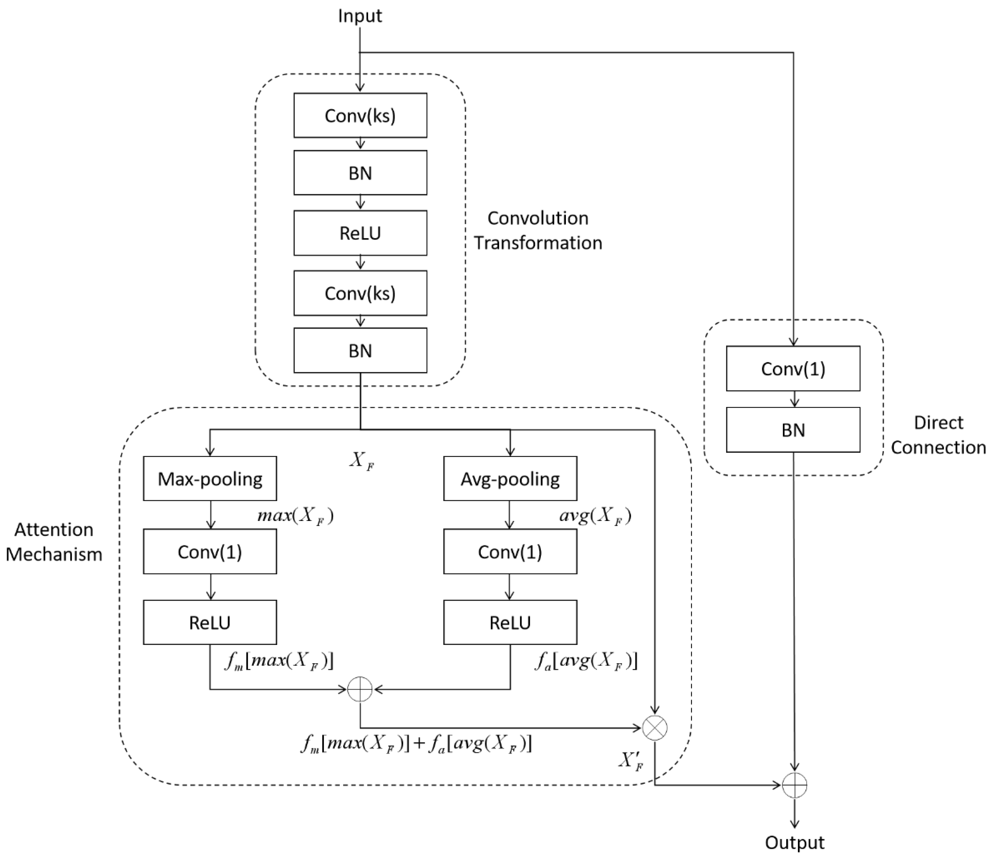
2.2.1. Average-Max Attention Residual Learning Block
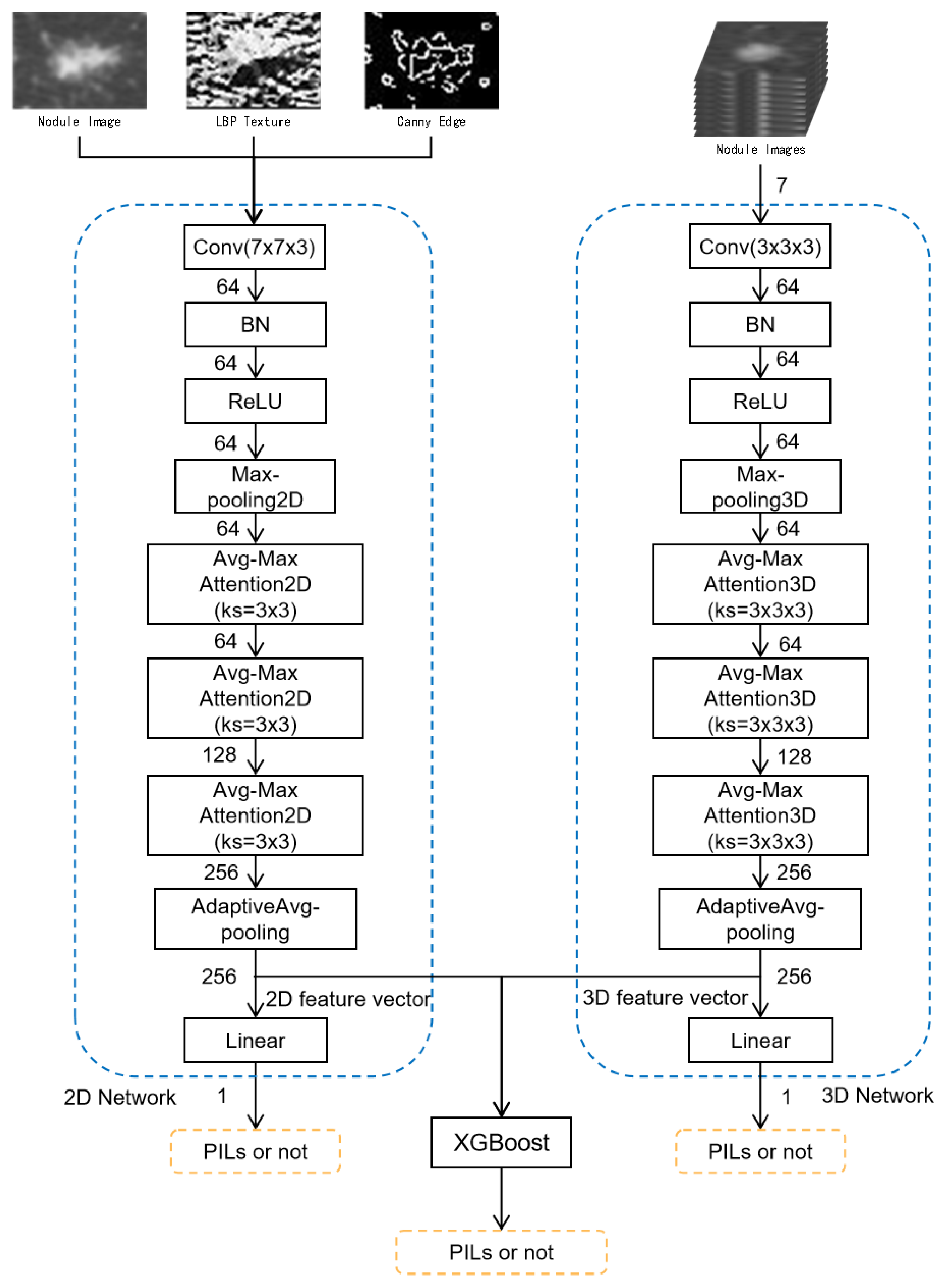
2.2.2. Multi-Level and Multi-Feature Hybrid Learning Network
3. Experiments and Results
3.1. Data Preparation
3.2. Model Evaluation
3.3. Training Preparation
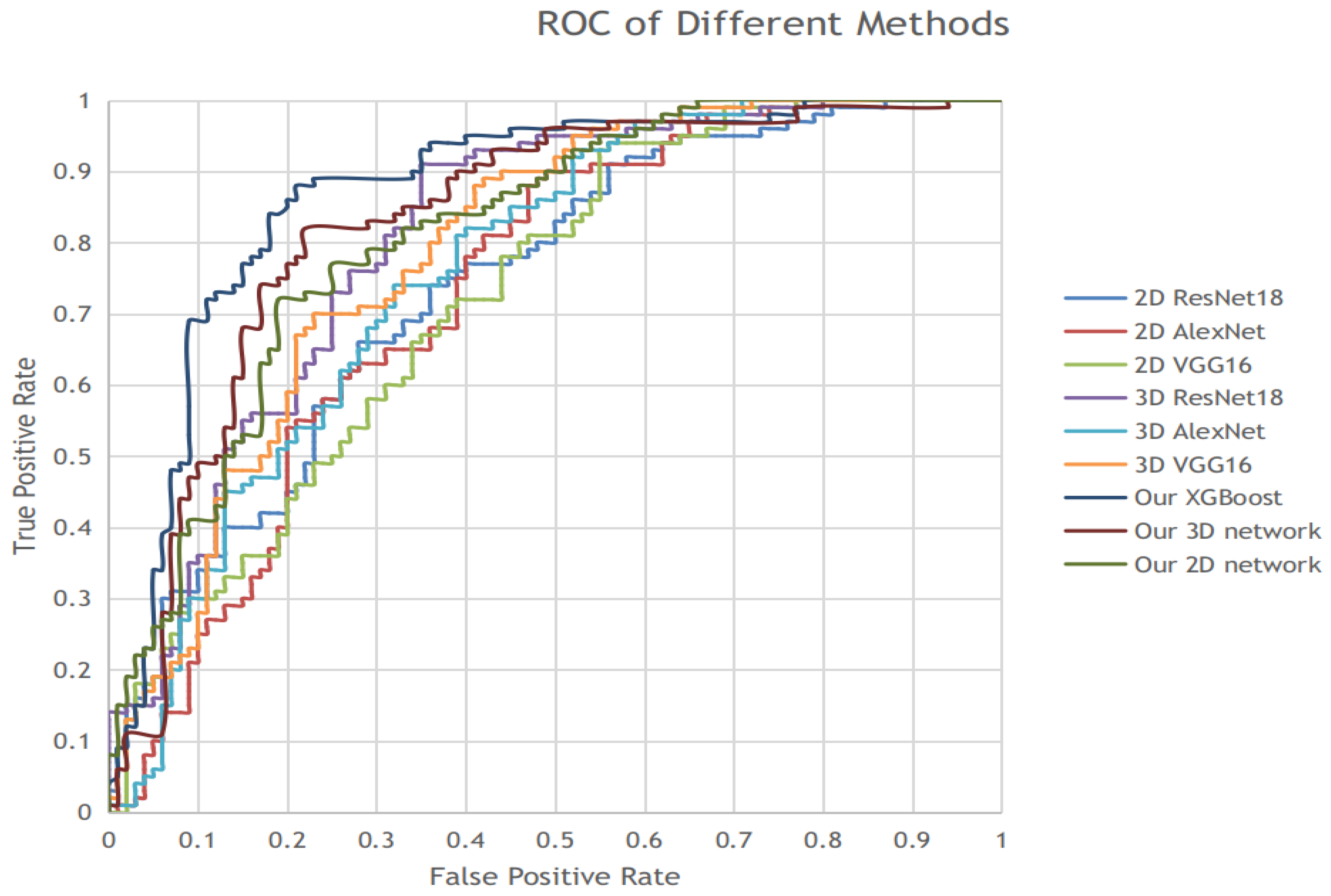
3.4. Results
4. Discussion
5. Conclusions
Author Contributions
Funding
Institutional Review Board Statement
Informed Consent Statement
Conflicts of Interest
References
- Siegel, R.L.; Miller, K.D.; Jemal, A. Cancer statistics, 2019. CA A Cancer J. Clin. 2019, 69, 7–34. [Google Scholar] [CrossRef] [PubMed]
- Travis, W.D.; Brambilla, E.; Noguchi, M.; Nicholson, A.G.; Geisinger, K.R.; Yatabe, Y.; Beer, D.G.; Powell, C.A.; Riely, G.J.; Van Schil, P.E.; et al. International association for the study of lung cancer/american thoracic society/european respiratory society international multidisciplinary classification of lung adenocarcinoma. J. Thorac. Oncol. 2011, 6, 244–285. [Google Scholar] [CrossRef] [PubMed]
- Bach, P.B.; Silvestri, G.A.; Hanger, M.; Jett, J.R. Screening for lung cancer: ACCP evidence-based clinical practice guidelines. Chest 2007, 132, 69S–77S. [Google Scholar] [CrossRef] [PubMed]
- Youlden, D.R.; Cramb, S.M.; Baade, P.D. The International Epidemiology of Lung Cancer: Geographical distribution and secular trends. J. Thorac. Oncol. 2008, 3, 819–831. [Google Scholar] [CrossRef] [PubMed]
- Smith, R.A.; Andrews, K.S.; Brooks, D.; Fedewa, S.A.; Manassaram-Baptiste, D.; Saslow, D.; Wender, R.C. Cancer screening in the United States, 2019: A review of current American Cancer Society guidelines and current issues in cancer screening. CA A Cancer J. Clin. 2019, 69, 184–210. [Google Scholar] [CrossRef] [PubMed]
- Bakator, M.; Radosav, D. Deep learning and medical diagnosis: A review of literature. Multimodal Technol. Interact. 2018, 2, 47. [Google Scholar] [CrossRef]
- Greenspan, H.; Van Ginneken, B.; Summers, R.M. Guest editorial deep learning in medical imaging: Overview and future promise of an exciting new technique. IEEE Trans. Med. Imaging 2016, 35, 1153–1159. [Google Scholar] [CrossRef]
- Sahiner, B.; Petzeshk, A.; Hadjiiski, L.M.; Wang, X.; Drukker, K.; Cha, K.H.; Summers, R.M.; Giger, M.L. Deep learning in medical imaging and radiation therapy. Med. Phys. 2019, 46, e1–e36. [Google Scholar] [CrossRef] [PubMed]
- Shen, W.; Zhou, M.; Yang, F.; Yang, C.; Tian, J. Multi-scale convolutional neural networks for lung nodule classification. In International Conference on Information Processing in Medical Imaging; Springer: Cham, Switzerland, 2015; pp. 588–599. [Google Scholar]
- Shen, W.; Zhou, M.; Yang, F.; Yu, D.; Dong, D.; Yang, C.; Zhang, Y.; Tian, J. Multi-crop convolutional neural networks for lung nodule malignancy suspiciousness classification. Pattern Recognit. 2017, 61, 663–673. [Google Scholar] [CrossRef]
- Al-Shabi, M.; Lan, B.L.; Chan, W.Y.; Ng, K.H.; Tan, M. Lung nodule classification using deep local–global networks. Int. J. Comput. Assist. Radiol. Surg. 2019, 14, 1815–1819. [Google Scholar] [CrossRef]
- Xu, X.; Wang, C.; Guo, J.; Gan, Y.; Wang, J.; Bai, H.; Zhang, L.; Li, W.; Yi, Z. MSCS-DeepLN: Evaluating lung nodule malignancy using multi-scale cost-sensitive neural networks. Med. Image Anal. 2020, 65, 101772. [Google Scholar] [CrossRef] [PubMed]
- Li, S.; Xu, P.; Li, B.; Chen, L.; Zhou, Z.; Hao, H.; Duan, Y.; Folkert, M.; Ma, J.; Huang, S.; et al. Predicting lung nodule malignancies by combining deep convolutional neural network and handcrafted features. Phys. Med. Biol. 2019, 64, 175012. [Google Scholar] [CrossRef] [PubMed]
- Srivastava, V.; Purwar, R.K. Classification of CT scan images of lungs using deep convolutional neural network with external shape-based features. J. Digit. Imaging 2020, 33, 252–261. [Google Scholar] [CrossRef] [PubMed]
- El-Regaily, S.A.; Salem, M.A.M.; Aziz, M.H.A.; Roushdy, M.I. Multi-view Convolutional Neural Network for lung nodule false positive reduction. Expert Syst. Appl. 2020, 162, 113017. [Google Scholar] [CrossRef]
- Ni, Y.; Yang, Y.; Zheng, D.; Xie, Z.; Huang, H.; Wang, W. The Invasiveness Classification of Ground-Glass Nodules Using 3D Attention Network and HRCT. J. Digit. Imaging 2020, 33, 1144–1154. [Google Scholar] [CrossRef] [PubMed]
- Lyu, J.; Bi, X.; Ling, S.H. Multi-level cross residual network for lung nodule classification. Sensors 2020, 20, 2837. [Google Scholar] [CrossRef] [PubMed]
- Sahlol, A.T.; Elaziz, M.A.; Jamal, A.T.; Damaeviius, R.; Hassan, O.F. A novel method for detection of tuberculosis in chest radiographs using artificial ecosystem-based optimisation of deep neural network features. Symmetry 2020, 12, 1146. [Google Scholar] [CrossRef]
- da Nobrega, R.V.M.; Rebouças Filho, P.P.; Rodrigues, M.B.; da Silva, S.P.; Junior, C.M.D.; de Albuquerque, V.H.C. Lung nodule malignancy classification in chest computed tomography images using transfer learning and convolutional neural networks. Neural Comput. Appl. 2020, 32, 11065–11082. [Google Scholar] [CrossRef]
- Capizzi, G.; Sciuto, G.L.; Napoli, C.; Poap, D.; Woniak, M. Small lung nodules detection based on fuzzy-logic and probabilistic neural network with bioinspired reinforcement learning. IEEE Trans. Fuzzy Syst. 2020, 28, 1178–1189. [Google Scholar] [CrossRef]
- Mnih, V.; Heess, N.; Graves, A.; Kavukcuoglu, K. Recurrent models of visual attention. arXiv 2014, arXiv:1406.6247. [Google Scholar]
- He, K.; Zhang, X.; Ren, S.; Sun, J. Deep residual learning for image recognition. In Proceedings of the IEEE conference on computer vision and pattern recognition, Las Vegas, NV, USA, 27–30 June 2016; pp. 770–778. [Google Scholar]
- Chen, T.; He, T.; Benesty, M.; Khotilovich, V.; Tang, Y.; Cho, H. Xgboost: Extreme gradient boosting. R Package Version 2015. [Google Scholar]
- Han, F.; Zhang, G.; Wang, H.; Song, B.; Lu, H.; Zhao, D.; Zhao, H.; Liang, Z. A texture feature analysis for diagnosis of pulmonary nodules using LIDC-IDRI database. In Proceedings of the 2013 IEEE International Conference on Medical Imaging Physics and Engineering, Shenyang, China, 19–20 October 2013; pp. 14–18. [Google Scholar]
- Heikkilä, M.; Pietikäinen, M.; Schmid, C. Description of interest regions with local binary patterns. Pattern Recognit. 2009, 42, 425–436. [Google Scholar] [CrossRef]
- Canny, J. A computational approach to edge detection. IEEE Trans. Pattern Anal. Mach. Intell. 1986, 6, 679–698. [Google Scholar] [CrossRef]
- Ruder, S. An overview of gradient descent optimization algorithms. arXiv 2016, arXiv:1609.04747. [Google Scholar]
- Yun, S.; Han, D.; Oh, S.J.; Chun, S.; Choe, J.; Yoo, Y. Cutmix: Regularization strategy to train strong classifiers with localizable features. In Proceedings of the IEEE/CVF International Conference on Computer Vision, Seoul, Korea, 27 October–2 November 2019; pp. 6023–6032. [Google Scholar]
- He, K.; Zhang, X.; Ren, S.; Sun, J. Delving deep into rectifiers: Surpassing human-level performance on imagenet classification. In Proceedings of the IEEE international conference on computer vision, Santiago, Chile, 7–13 December 2015; pp. 1026–1034. [Google Scholar]


| Models | Accuracy | Sensitivity | Specificity | F1 Score | AUC |
|---|---|---|---|---|---|
| 2D Network | 0.75 | 0.79 | 0.71 | 0.76 | 0.81 |
| 3D Network | 0.785 | 0.82 | 0.75 | 0.79 | 0.83 |
| XGBoost | 0.83 | 0.86 | 0.8 | 0.83 | 0.88 |
| Predicted Class | |||
| Positive | Negative | ||
| Actual Class | Positive | 86 | 14 |
| Negative | 20 | 80 | |
| Models | Accuracy | Sensitivity | Specificity | F1 Score | AUC |
|---|---|---|---|---|---|
| Without CutMix | 0.81 | 0.81 | 0.81 | 0.81 | 0.87 |
| With CutMix | 0.83 | 0.86 | 0.8 | 0.83 | 0.88 |
| Models | Accuracy | Sensitivity | Specificity | F1 Score | AUC |
|---|---|---|---|---|---|
| 2D VGG16 | 0.655 | 0.66 | 0.66 | 0.65 | 0.72 |
| 2D AlexNet | 0.675 | 0.63 | 0.69 | 0.66 | 0.73 |
| 2D ResNet18 | 0.68 | 0.66 | 0.70 | 0.67 | 0.73 |
| Our 2D network | 0.75 | 0.79 | 0.71 | 0.76 | 0.81 |
| 3D VGG16 | 0.72 | 0.82 | 0.62 | 0.74 | 0.79 |
| 3D AlexNet | 0.69 | 0.77 | 0.61 | 0.71 | 0.76 |
| 3D ResNet18 | 0.75 | 0.81 | 0.69 | 0.76 | 0.81 |
| Our 3D Network | 0.785 | 0.82 | 0.75 | 0.79 | 0.83 |
| XGBoost | 0.83 | 0.86 | 0.8 | 0.83 | 0.88 |
Publisher’s Note: MDPI stays neutral with regard to jurisdictional claims in published maps and institutional affiliations. |
© 2021 by the authors. Licensee MDPI, Basel, Switzerland. This article is an open access article distributed under the terms and conditions of the Creative Commons Attribution (CC BY) license (https://creativecommons.org/licenses/by/4.0/).
Share and Cite
Fan, J.; Bao, J.; Xu, J.; Mo, J. Multi-Dimension and Multi-Feature Hybrid Learning Network for Classifying the Sub Pathological Type of Lung Nodules through LDCT. Sensors 2021, 21, 2734. https://doi.org/10.3390/s21082734
Fan J, Bao J, Xu J, Mo J. Multi-Dimension and Multi-Feature Hybrid Learning Network for Classifying the Sub Pathological Type of Lung Nodules through LDCT. Sensors. 2021; 21(8):2734. https://doi.org/10.3390/s21082734
Chicago/Turabian StyleFan, Jiacheng, Jianying Bao, Jianlin Xu, and Jinqiu Mo. 2021. "Multi-Dimension and Multi-Feature Hybrid Learning Network for Classifying the Sub Pathological Type of Lung Nodules through LDCT" Sensors 21, no. 8: 2734. https://doi.org/10.3390/s21082734
APA StyleFan, J., Bao, J., Xu, J., & Mo, J. (2021). Multi-Dimension and Multi-Feature Hybrid Learning Network for Classifying the Sub Pathological Type of Lung Nodules through LDCT. Sensors, 21(8), 2734. https://doi.org/10.3390/s21082734