
Subsentence Extraction from Text Using Coverage-Based Deep Learning Language Models

 ,
,  , and
, and
Abstract
1. Introduction
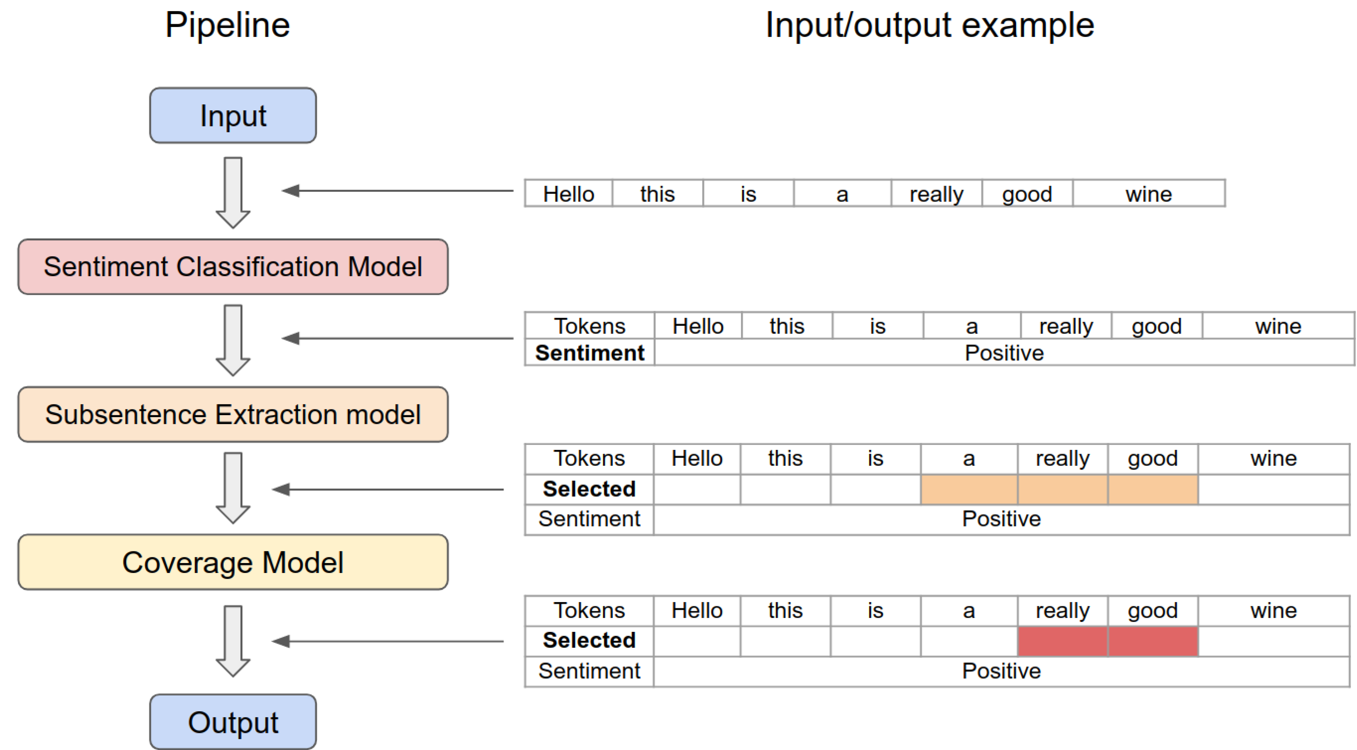
- Proposing a novel coverage-based subsentence extraction system that takes into considerations the length of subsentence and an end-to-end pipeline that can be directly leveraged by Human-Robot Interaction;
- Performing intensive qualitative and quantitative evaluations of sentiment classification and subsentence extraction
- Returning lessons learnt to the community as a form of open dataset and source code (https://github.com/UoA-CARES/BuilT-NLP, accessed on 20 April 2021).
2. Related Work
2.1. Natural Language Processing for Sentiment Analysis
2.2. Emotion Detection in Sentiment Analysis
2.3. Human–Robot Interaction
3. Methodologies
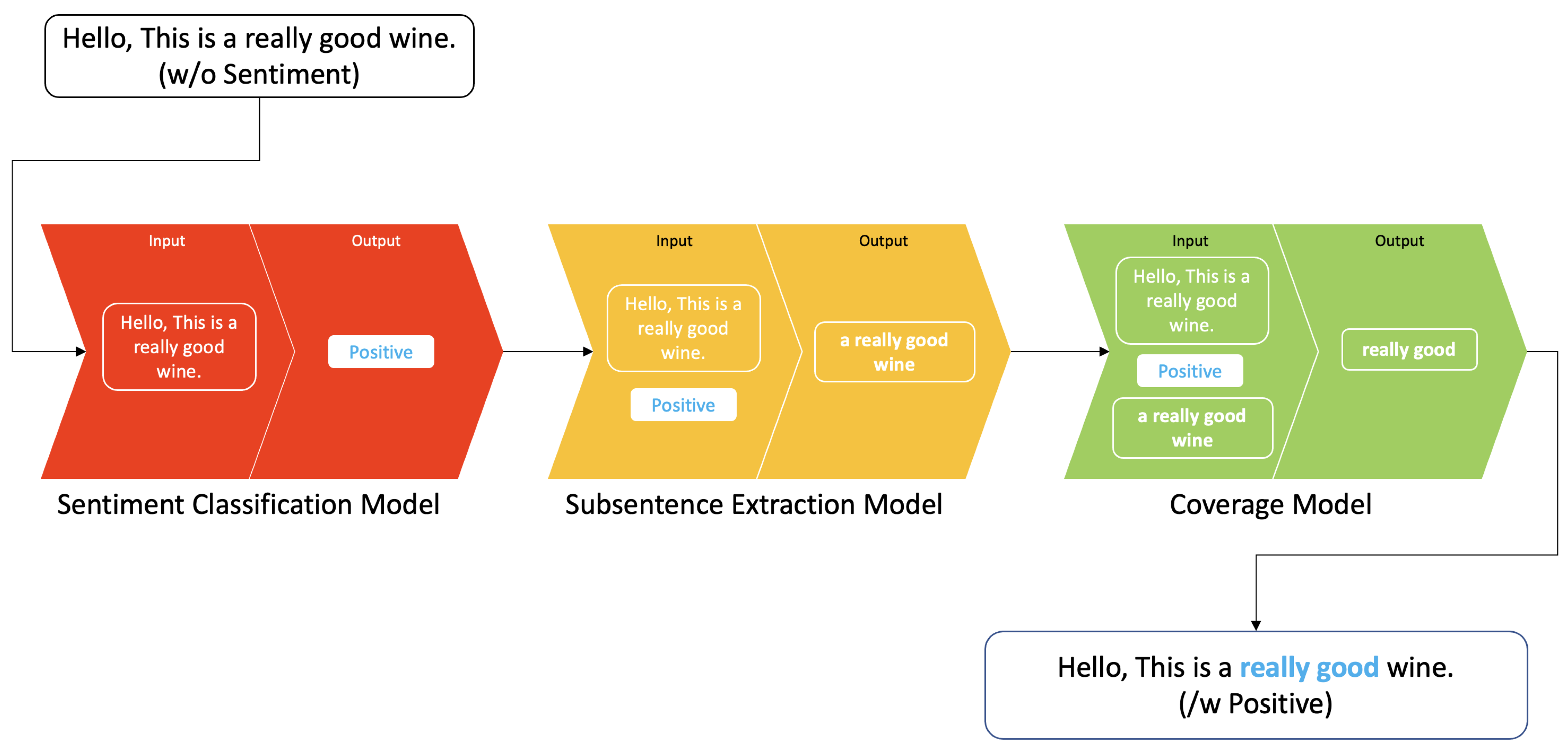
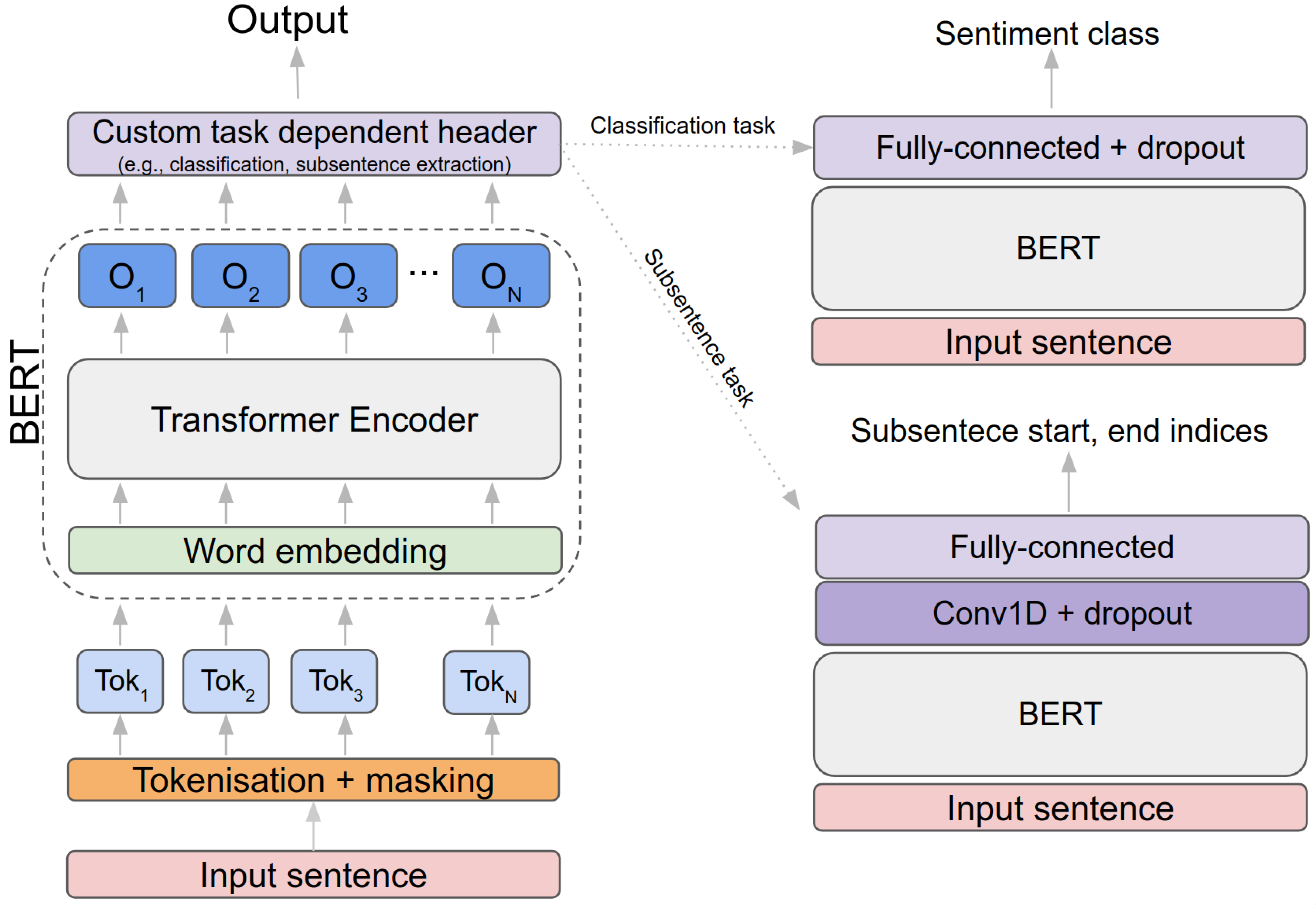
3.1. BERT and RoBERTa Transformer Language Models
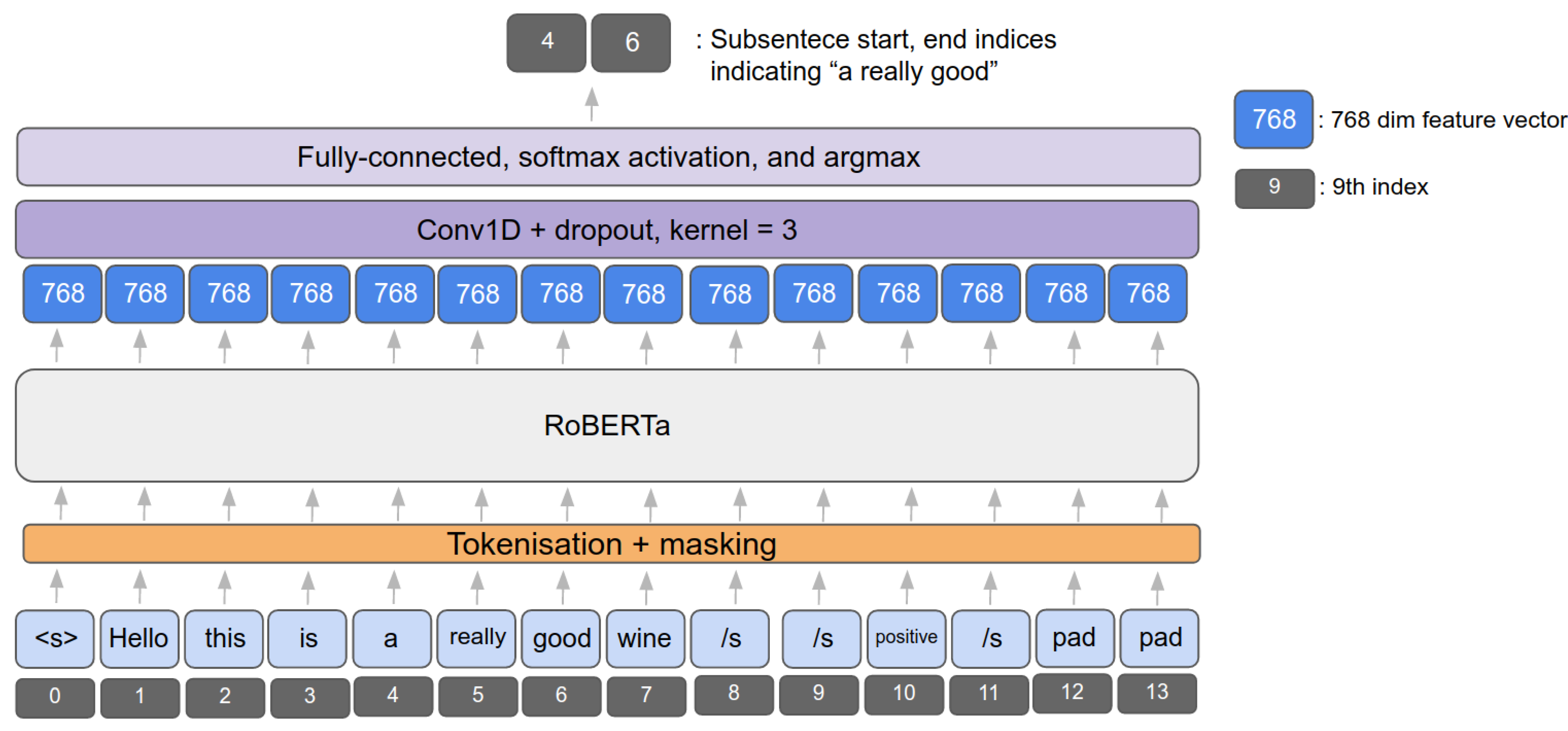
3.2. Sentiment Classification
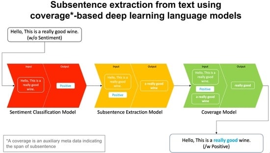
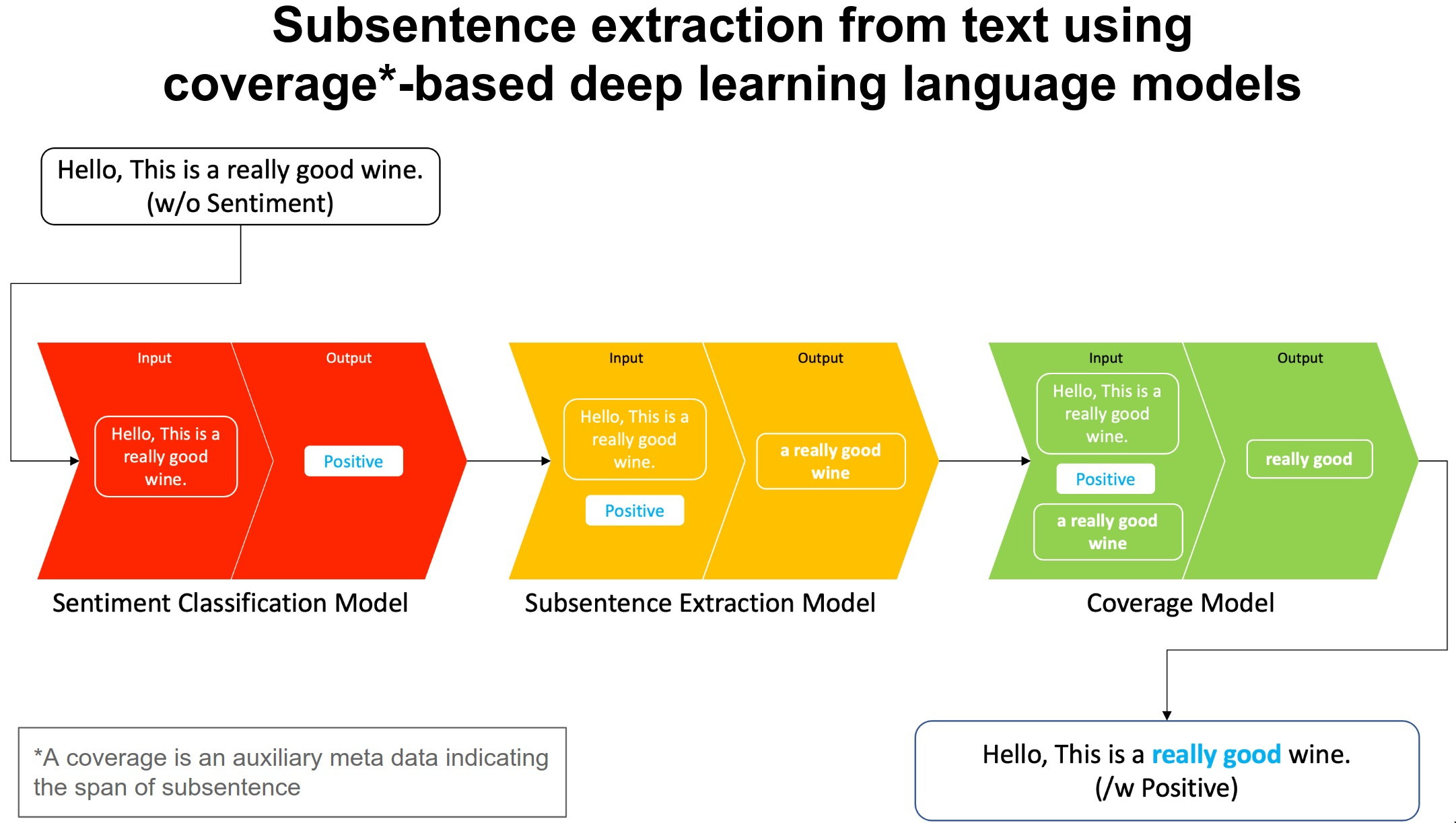
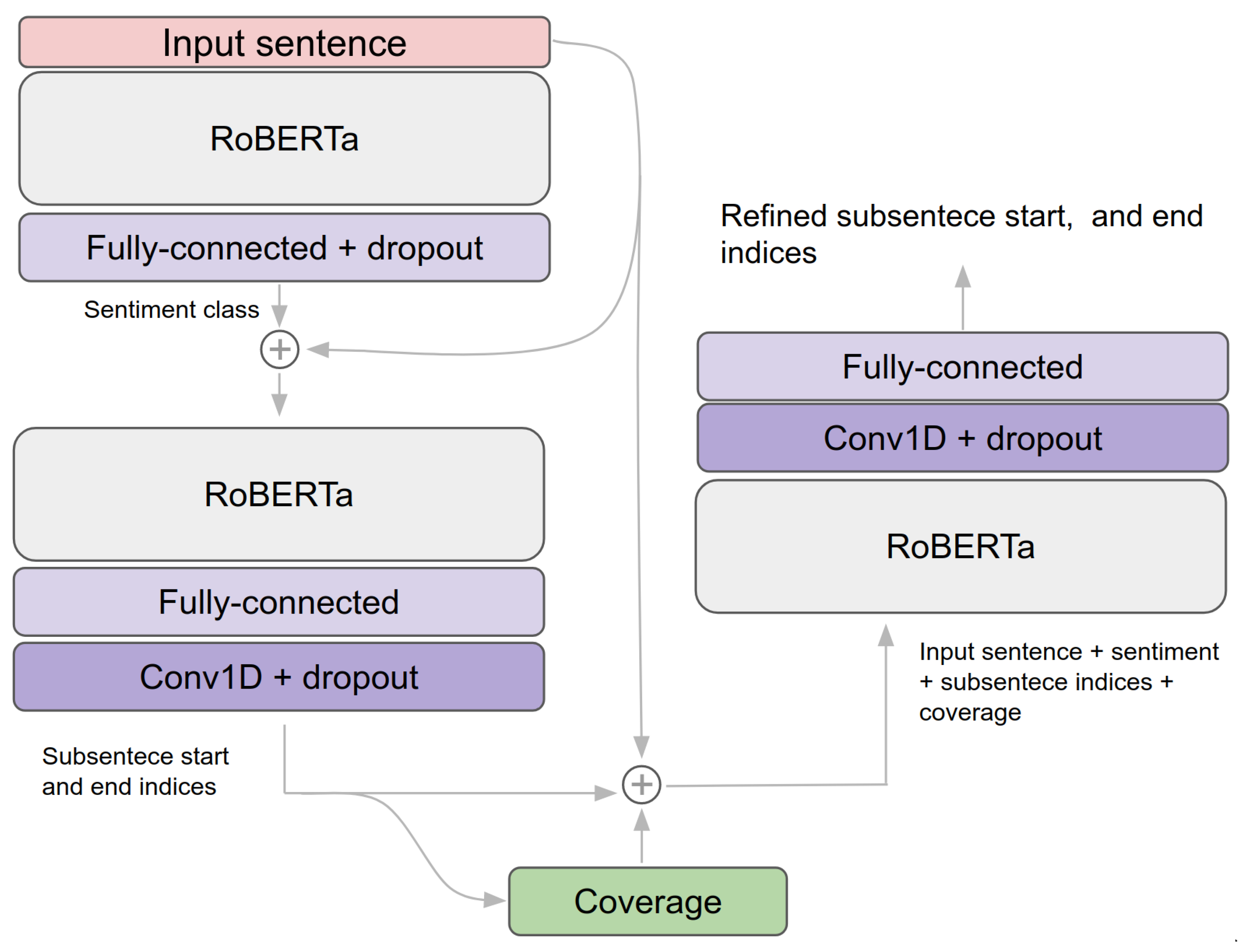
3.3. Coverage Model for Subsentence Extraction
| Algorithm 1: Coverage-based subsentence extraction algorithm. |
 |
3.4. End-To-End Sentiment and Subsentence Extraction Pipeline
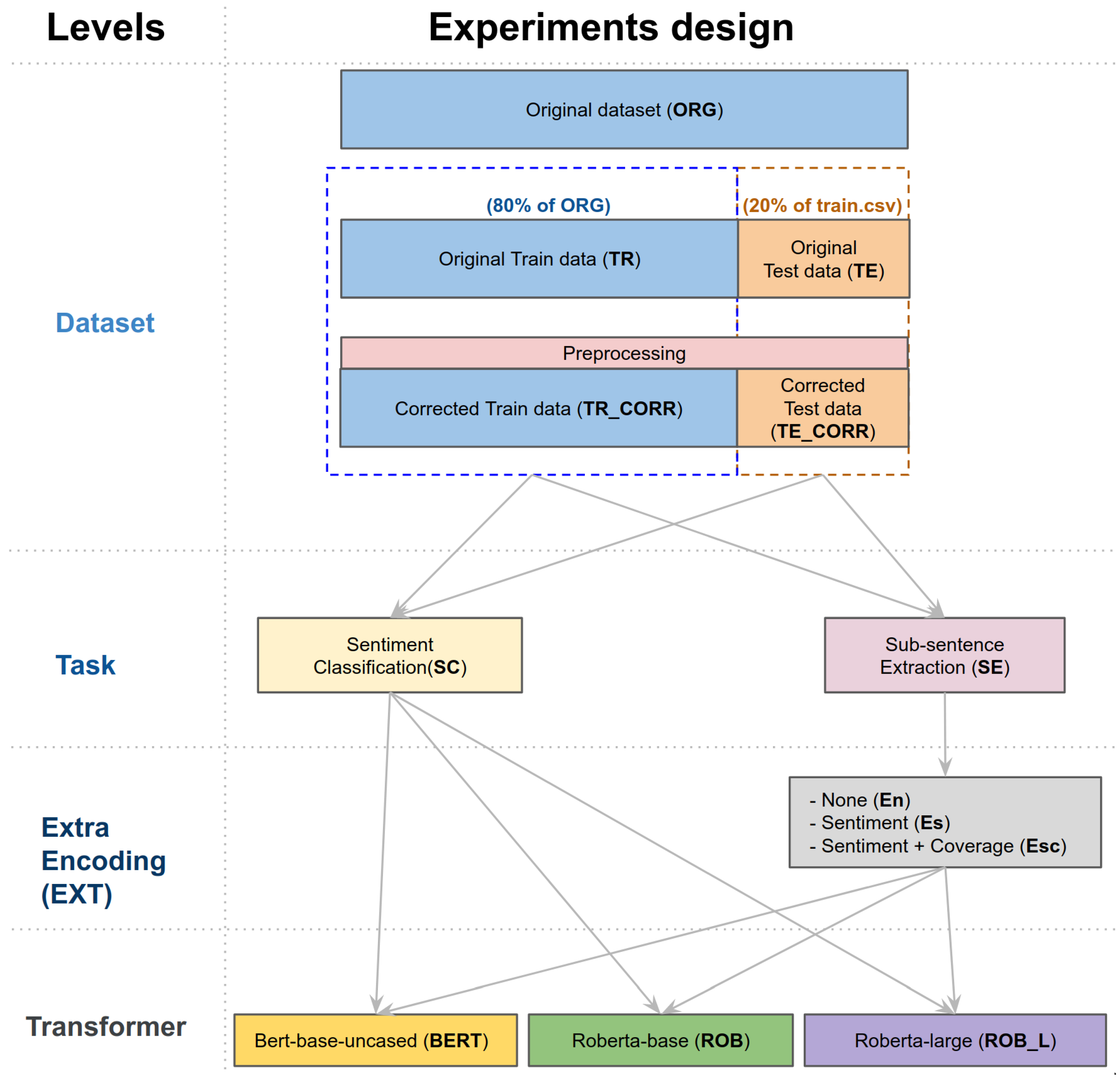
4. Dataset and Experiments Design
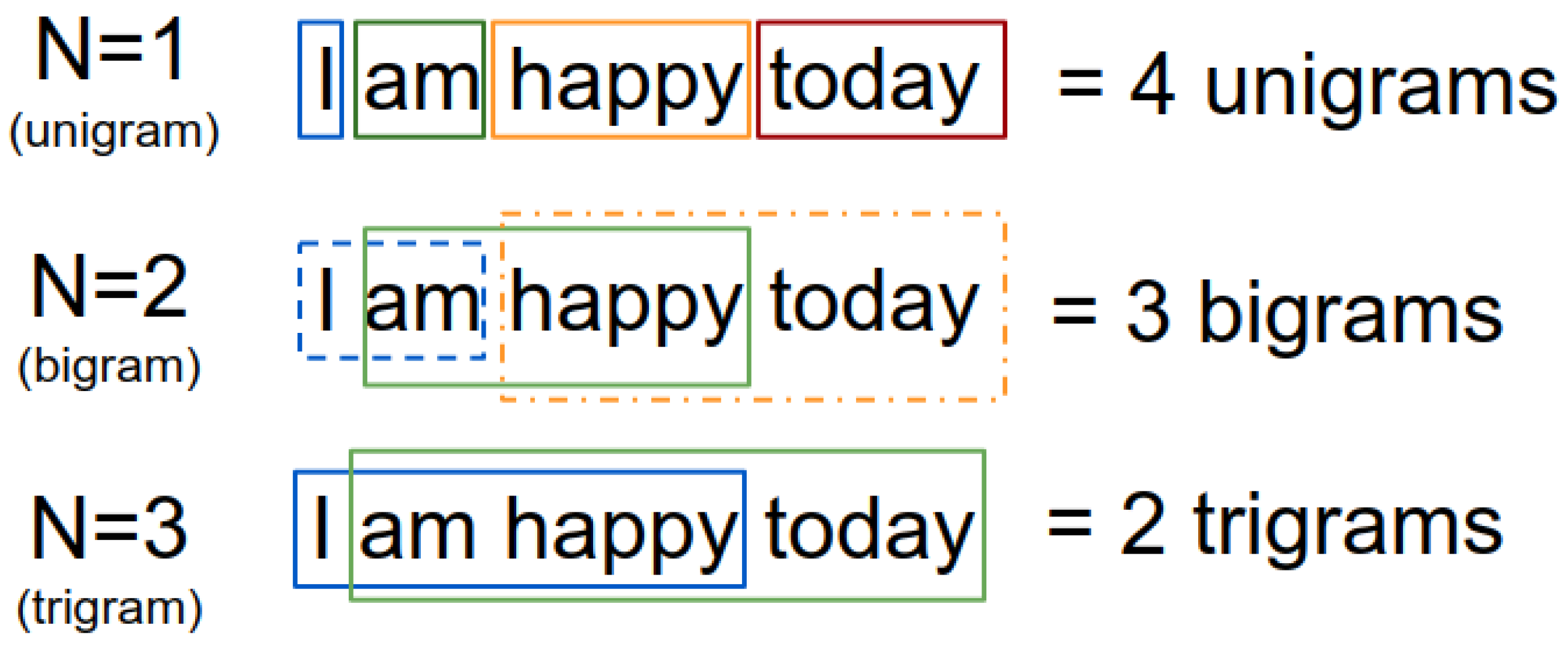
4.1. Tokenisation and Input Data Preprocessing
4.2. Tweet Sentiment Dataset
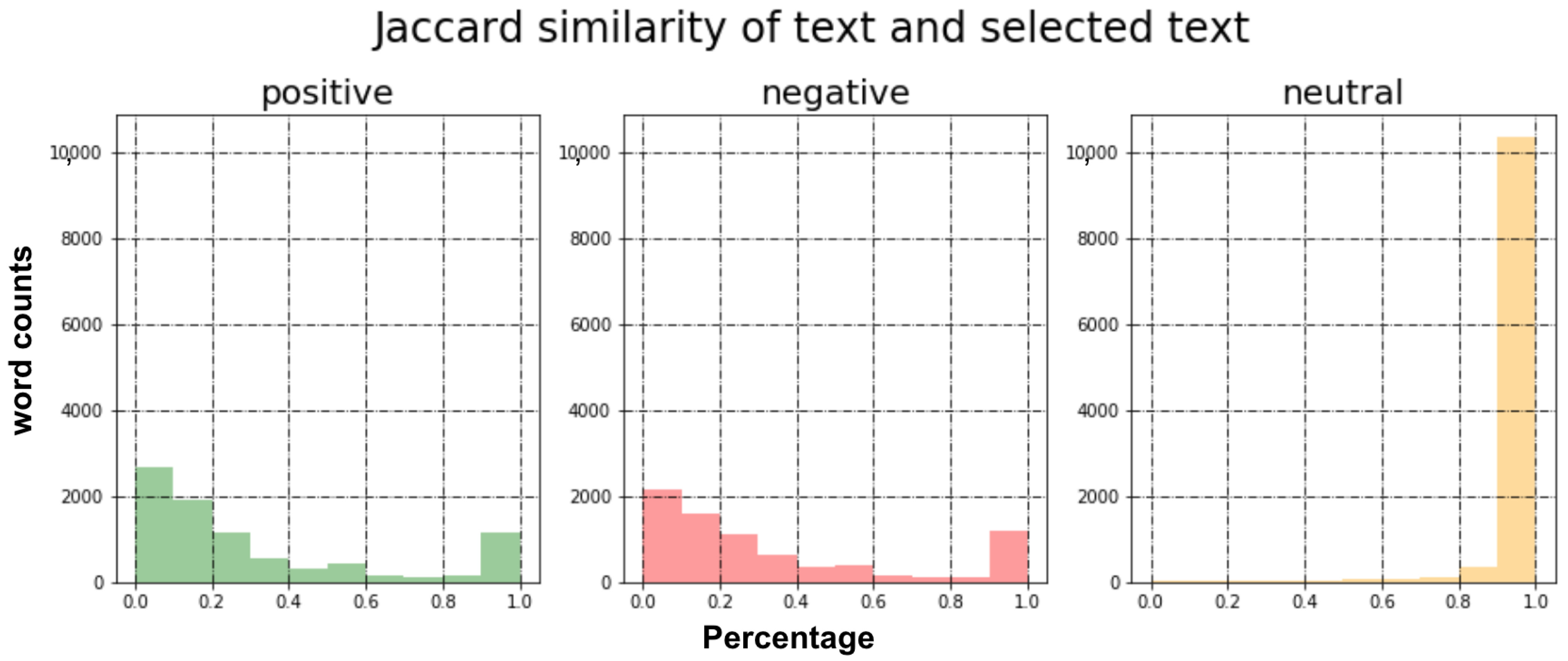
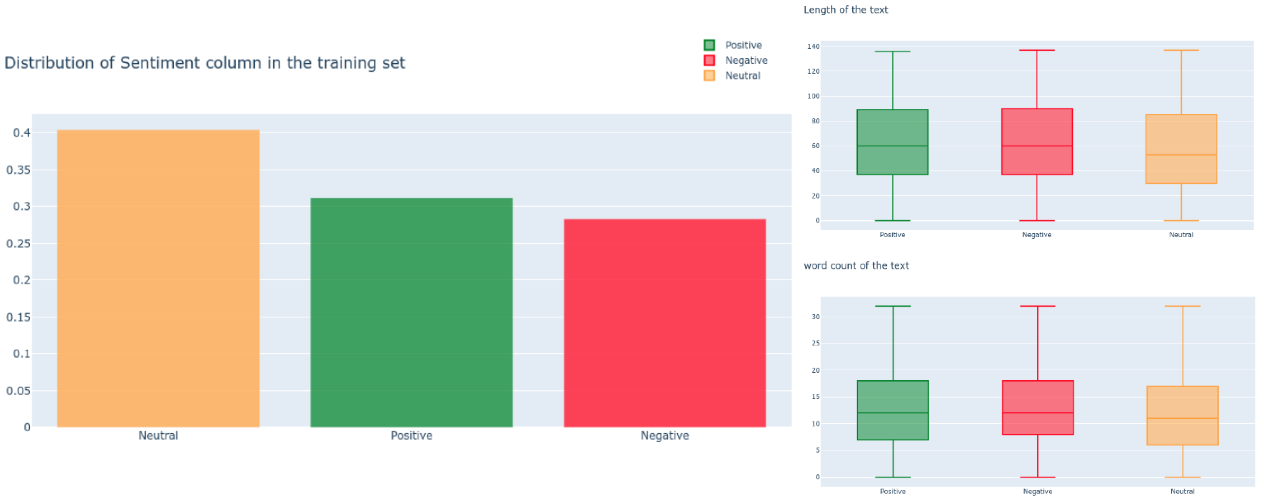
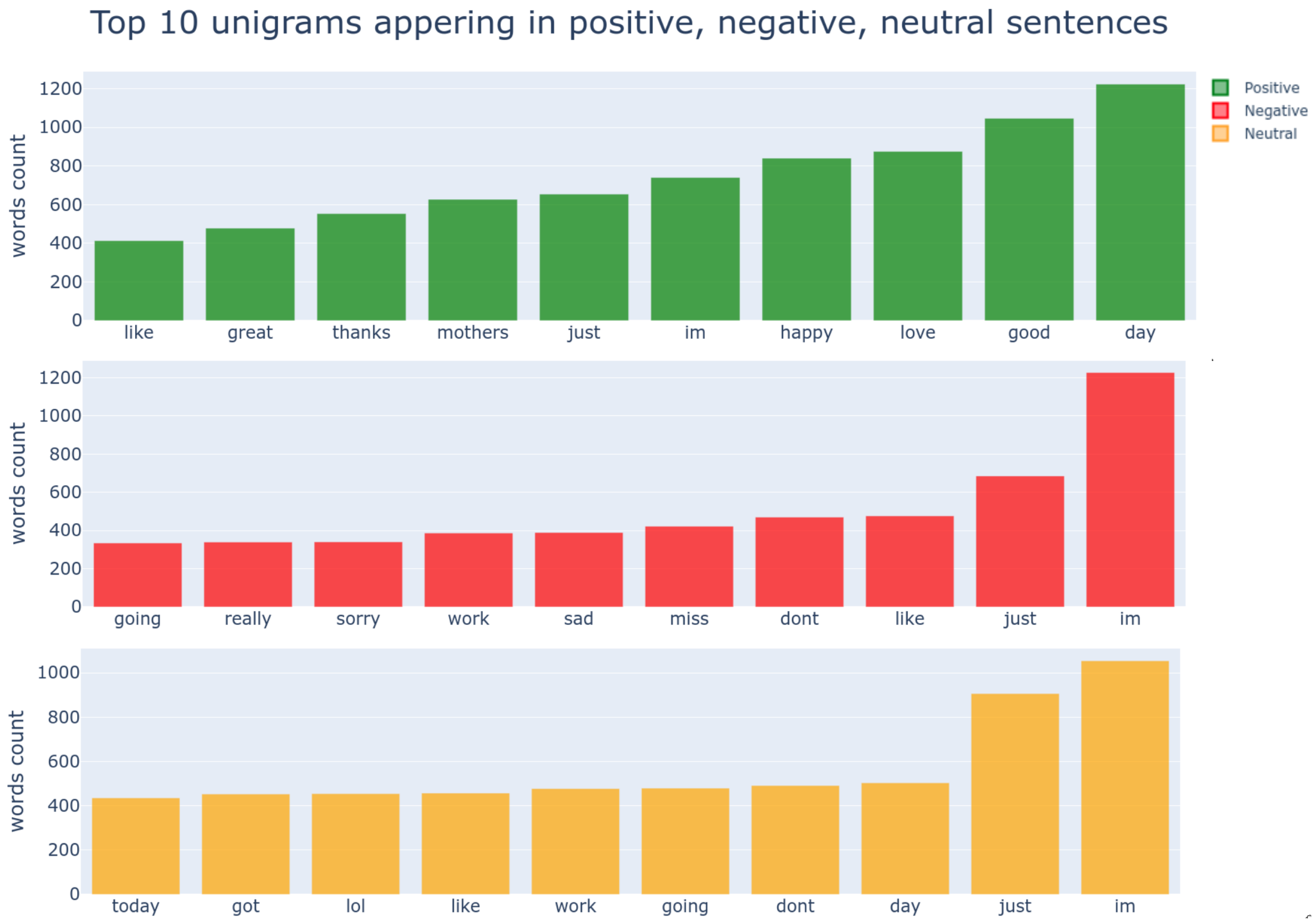
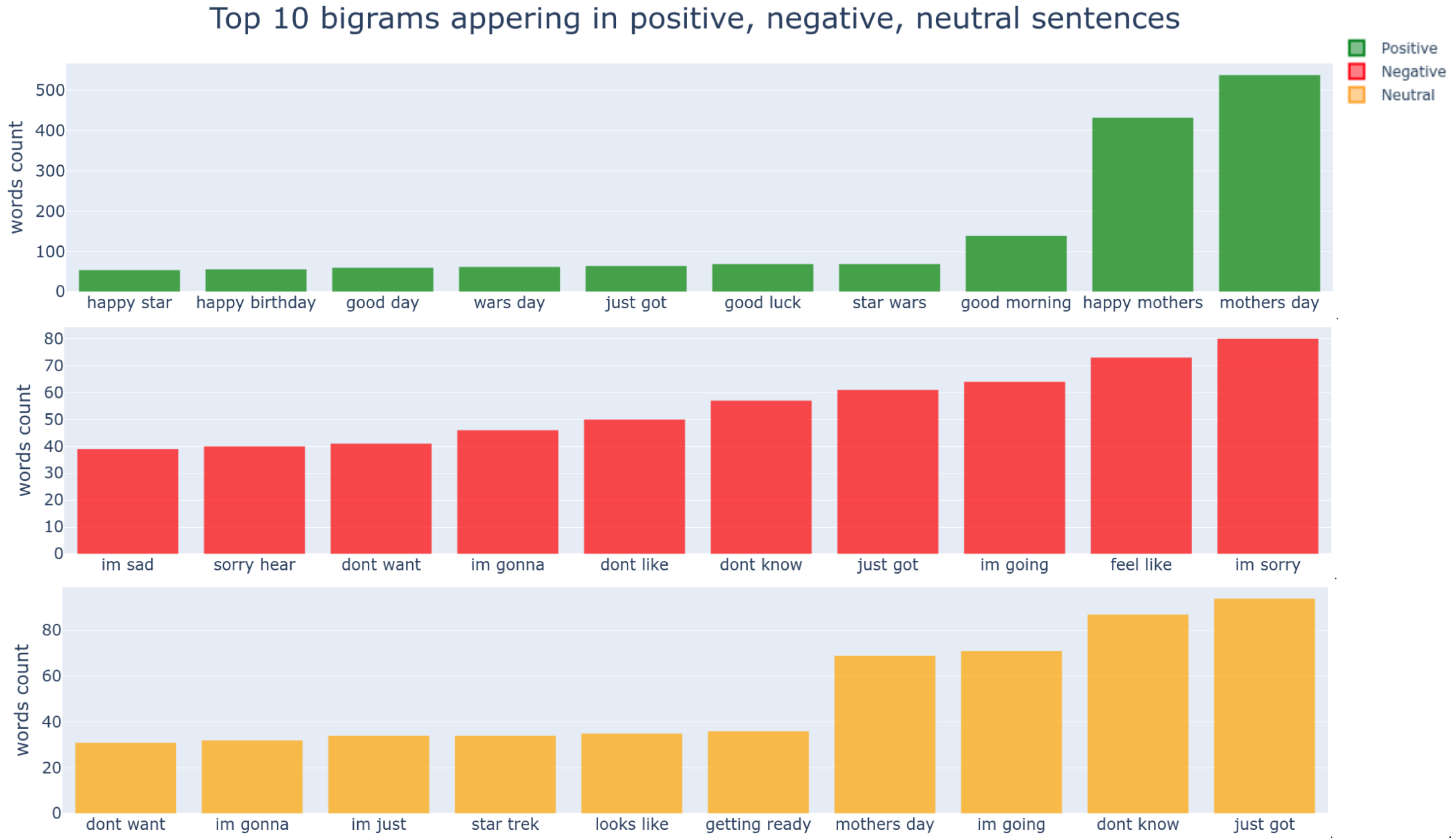
4.3. Exploratory Data Analysis (EDA)
4.4. Dataset Preparation
5. Model Training
5.1. Model Details
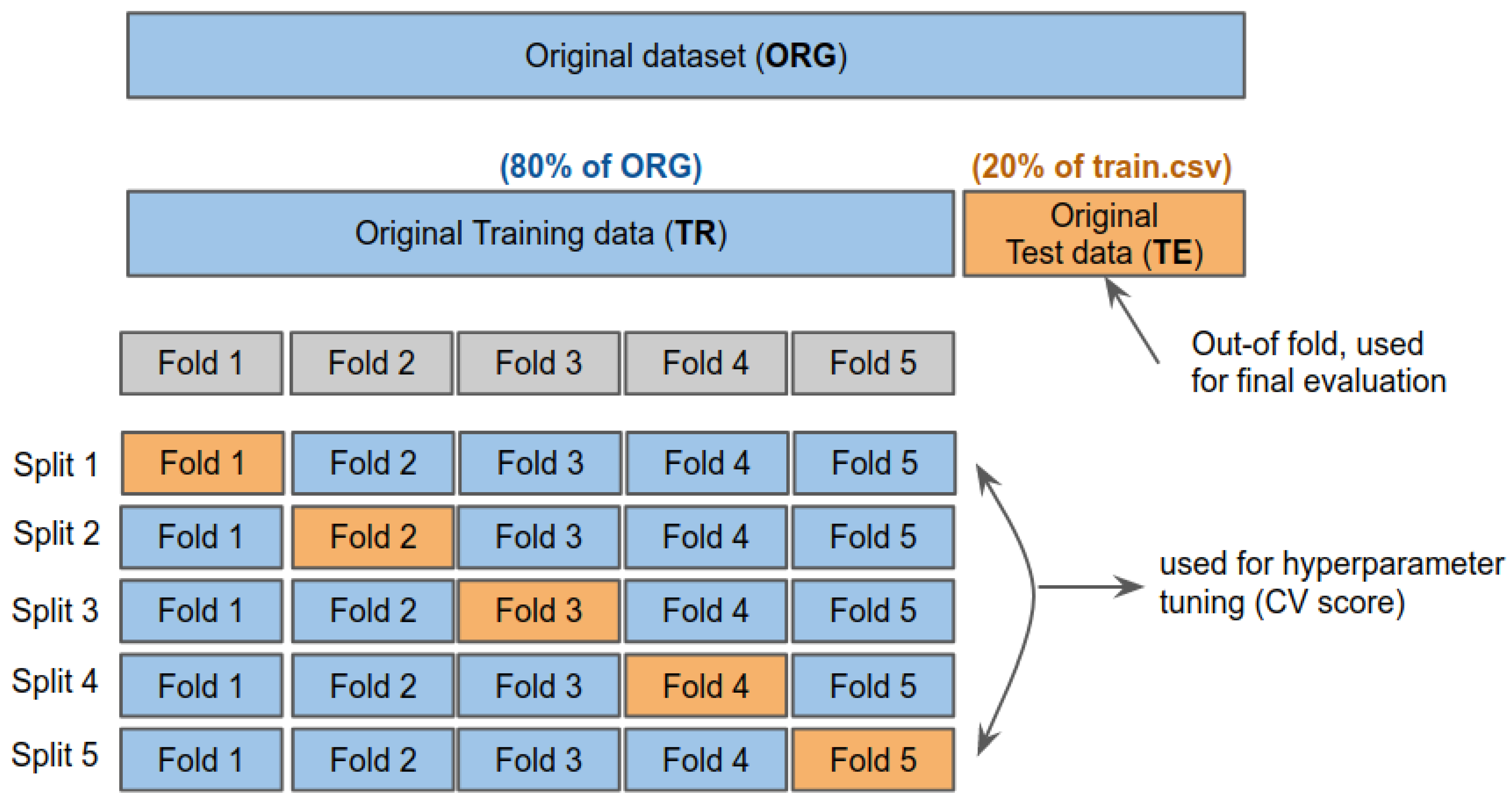
5.2. K-Fold Cross Validation
5.3. Training Configuration
6. Experimental Results
6.1. Evaluation Metrics
6.1.1. Area-Under-the-Curve
6.1.2. Harmonic Score
6.1.3. Jaccard Score for Subsentence Extraction
6.2. Model Ensemble
6.3. Classification Results
6.4. Coverage-Based Subsentence Extraction
6.5. End-to-End Pipeline Evaluation Results
6.6. Class Activation Mapping
7. Discussion and Limitations
8. Conclusions
Author Contributions
Funding
Institutional Review Board Statement
Informed Consent Statement
Data Availability Statement
Acknowledgments
Conflicts of Interest
Abbreviations
| AI | Artificial Intelligence |
| AUC | Area-Under-the Curve |
| BERT | Bidirectional Encoder Representations from Transformers |
| BPE | Byte-Pair Encoding |
| CAM | Class Activation Mapping |
| CEL | Cross-Entropy Loss |
| CV | Cross-Validation |
| EDA | Exploratory Data Analysis52 |
| GLUE | General Language Understanding Evaluation |
| GPT-3 | Generative Pre-trained63Transformer 3 |
| HRI | Human–Robot Interaction |
| NLP | Natural Language Processing |
| NSP | Next Sentence Prediction |
| RoBERTa | A Robustly Optimized BERT Pretraining Approach |
| S2E | Sentence To Emotion |
| SOTA | State-Of-The-Art |
| SSML | Speech Synthesis Markup Language |
| SQuAD | Stanford Question Answering Dataset |
References
- Liu, B.; Zhang, L. A survey of opinion mining and sentiment analysis. In Mining Text Data; Springer: Berlin/Heidelberg, Germany, 2012; pp. 415–463. [Google Scholar]
- Lee, M.; Forlizzi, J.; Kiesler, S.; Rybski, P.; Antanitis, J.; Savetsila, S. Personalization in HRI: A Longitudinal Field Experiment. In Proceedings of the ACM/IEEE International Conference on Human-Robot Interaction, Boston, MA, USA, 5–8 March 2012. [Google Scholar]
- Clabaugh, C.; Mahajan, K.; Jain, S.; Pakkar, R.; Becerra, D.; Shi, Z.; Deng, E.; Lee, R.; Ragusa, G.; Mataric, M. Long-Term Personalization of an In-Home Socially Assistive Robot for Children With Autism Spectrum Disorders. Front. Robot. AI 2019, 6, 110. [Google Scholar] [CrossRef]
- Di Nuovo, A.; Broz, F.; Wang, N.; Belpaeme, T.; Cangelosi, A.; Jones, R.; Esposito, R.; Cavallo, F.; Dario, P. The multi-modal interface of Robot-Era multi-robot services tailored for the elderly. Intell. Serv. Robot. 2018, 11, 109–126. [Google Scholar] [CrossRef]
- Henkemans, O.; Bierman, B.; Janssen, J.; Neerincx, M.; Looije, R.; van der Bosch, H.; van der Giessen, J. Using a robot to personalise health education for children with diabetes type 1: A pilot study. Patient Educ. Couns. 2013, 92, 174–181. [Google Scholar] [CrossRef] [PubMed]
- Fong, T.; Nourbakhsh, I.; Dautenhahn, K. A survey of socially interactive robots. Robot. Auton. Syst. 2003, 42, 143–166. [Google Scholar] [CrossRef]
- Acheampong, F.A.; Wenyu, C.; Nunoo-Mensah, H. Text-based emotion detection: Advances, challenges, and opportunities. Eng. Rep. 2020, 2, 1. [Google Scholar] [CrossRef]
- Ahn, H.S.; Lee, D.W.; Choi, D.; Lee, D.Y.; Hur, M.; Lee, H. Uses of facial expressions of android head system according to gender and age. In Proceedings of the IEEE International Conference on Systems, Man, and Cybernetics (SMC), Seoul, Korea, 14–17 October 2012; pp. 2300–2305. [Google Scholar]
- Brown, T.B.; Mann, B.; Ryder, N.; Subbiah, M.; Kaplan, J.; Dhariwal, P.; Neelakantan, A.; Shyam, P.; Sastry, G.; Askell, A.; et al. Language models are few-shot learners. arXiv 2020, arXiv:2005.14165. [Google Scholar]
- Pennington, J.; Socher, R.; Manning, C.D. Glove: Global vectors for word representation. In Proceedings of the 2014 Conference on Empirical Methods in Natural Language Processing (EMNLP), Doha, Qatar, 25–29 October 2014; pp. 1532–1543. [Google Scholar]
- Johnson, M.; Schuster, M.; Le, Q.V.; Krikun, M.; Wu, Y.; Chen, Z.; Thorat, N.; Viégas, F.; Wattenberg, M.; Corrado, G.; et al. Google’s multilingual neural machine translation system: Enabling zero-shot translation. Trans. Assoc. Comput. Linguist. 2017, 5, 339–351. [Google Scholar] [CrossRef]
- Cui, Y.; Chen, Z.; Wei, S.; Wang, S.; Liu, T.; Hu, G. Attention-over-attention neural networks for reading comprehension. arXiv 2016, arXiv:1607.04423. [Google Scholar]
- Soares, M.A.C.; Parreiras, F.S. A literature review on question answering techniques, paradigms and systems. J. King Saud Univ. Comput. Inf. Sci. 2020, 32, 635–646. [Google Scholar]
- Rajpurkar, P.; Jia, R.; Liang, P. Know what you do not know: Unanswerable questions for SQuAD. arXiv 2018, arXiv:1806.03822. [Google Scholar]
- Rajpurkar, P.; Zhang, J.; Lopyrev, K.; Liang, P. Squad: 100,000+ questions for machine comprehension of text. arXiv 2016, arXiv:1606.05250. [Google Scholar]
- Zhou, W.; Zhang, X.; Jiang, H. Ensemble BERT with Data Augmentation and Linguistic Knowledge on SQuAD 2.0. Tech. Rep. 2019. [Google Scholar]
- Wang, A.; Singh, A.; Michael, J.; Hill, F.; Levy, O.; Bowman, S.R. GLUE: A multi-task benchmark and analysis platform for natural language understanding. arXiv 2018, arXiv:1804.07461. [Google Scholar]
- Lai, G.; Xie, Q.; Liu, H.; Yang, Y.; Hovy, E. Race: Large-scale reading comprehension dataset from examinations. arXiv 2017, arXiv:1704.04683. [Google Scholar]
- Crnic, J. Introduction to Modern Information Retrieval. Libr. Manag. 2011, 32, 373–374. [Google Scholar] [CrossRef]
- Cambria, E.; Das, D.; Bandyopadhyay, S.; Feraco, A. Affective computing and sentiment analysis. In A Practical Guide to Sentiment Analysis; Springer: Berlin/Heidelberg, Germany, 2017; pp. 1–10. [Google Scholar]
- Kanakaraj, M.; Guddeti, R.M.R. Performance analysis of Ensemble methods on Twitter sentiment analysis using NLP techniques. In Proceedings of the 2015 IEEE 9th International Conference on Semantic Computing (IEEE ICSC 2015), Anaheim, CA, USA, 7–9 February 2015; pp. 169–170. [Google Scholar]
- Guo, X.; Li, J. A novel twitter sentiment analysis model with baseline correlation for financial market prediction with improved efficiency. In Proceedings of the Sixth International Conference on Social Networks Analysis, Management and Security (SNAMS), Granada, Spain, 22–25 October 2019; pp. 472–477. [Google Scholar]
- Devlin, J.; Chang, M.W.; Lee, K.; Toutanova, K. Bert: Pre-training of deep bidirectional transformers for language understanding. arXiv 2018, arXiv:1810.04805. [Google Scholar]
- Liu, Y.; Ott, M.; Goyal, N.; Du, J.; Joshi, M.; Chen, D.; Levy, O.; Lewis, M.; Zettlemoyer, L.; Stoyanov, V. Roberta: A robustly optimized bert pretraining approach. arXiv 2019, arXiv:1907.11692. [Google Scholar]
- Szabóová, M.; Sarnovský, M.; Maslej Krešňáková, V.; Machová, K. Emotion Analysis in Human–Robot Interaction. Electronics 2020, 9, 1761. [Google Scholar] [CrossRef]
- De Albornoz, J.C.; Plaza, L.; Gervás, P. SentiSense: An easily scalable concept-based affective lexicon for sentiment analysis. In LREC; European Language Resources Association (ELRA): Luxembourg, 2012; Volume 12, pp. 3562–3567. [Google Scholar]
- Ekman, P. Expression and the nature of emotion. Approaches Emot. 1984, 3, 344. [Google Scholar]
- Amado-Boccara, I.; Donnet, D.; Olié, J. The concept of mood in psychology. L’encephale 1993, 19, 117–122. [Google Scholar]
- Breazeal, C. Emotion and sociable humanoid robots. Int. J. Hum. Comput. Stud. 2003, 59, 119–155. [Google Scholar] [CrossRef]
- Striepe, H.; Lugrin, B. There once was a robot storyteller: Measuring the effects of emotion and non-verbal behaviour. In International Conference on Social Robotics, Proceedings of the 9th International Conference, ICSR 2017, Tsukuba, Japan, 22–24 November 2017; Springer: Berlin/Heidelberg, Germany, 2017; pp. 126–136. [Google Scholar]
- Shen, J.; Rudovic, O.; Cheng, S.; Pantic, M. Sentiment apprehension in human–robot interaction with NAO. In Proceedings of the International Conference on Affective Computing and Intelligent Interaction (ACII), Xi’an, China, 21–24 September 2015; pp. 867–872. [Google Scholar]
- Bae, B.C.; Brunete, A.; Malik, U.; Dimara, E.; Jermsurawong, J.; Mavridis, N. Towards an empathizing and adaptive storyteller system. In Proceedings of the AAAI Conference on Artificial Intelligence and Interactive Digital Entertainment, Stanford, CA, USA, 8–12 October 2012; Volume 8. [Google Scholar]
- Rodriguez, I.; Martínez-Otzeta, J.M.; Lazkano, E.; Ruiz, T. Adaptive emotional chatting behavior to increase the sociability of robots. In International Conference on Social Robotics, Proceedings of the 9th International Conference, ICSR 2017, Tsukuba, Japan, 22–24 November 2017; Springer: Berlin/Heidelberg, Germany, 2017; pp. 666–675. [Google Scholar]
- Paradeda, R.; Ferreira, M.J.; Martinho, C.; Paiva, A. Would You Follow the Suggestions of a Storyteller Robot? In International Conference on Interactive Digital Storytelling, Proceedings of the 11th International Conference on Interactive Digital Storytelling, ICIDS 2018, Dublin, Ireland, 5–8 December 2018; Springer: Berlin/Heidelberg, Germany, 2018; pp. 489–493. [Google Scholar]
- Vaswani, A.; Shazeer, N.; Parmar, N.; Uszkoreit, J.; Jones, L.; Gomez, A.N.; Kaiser, U.; Polosukhin, I. Attention is All you Need. In Advances in Neural Information Processing Systems 30; Guyon, I., Luxburg, U.V., Bengio, S., Wallach, H., Fergus, R., Vishwanathan, S., Garnett, R., Eds.; Curran Associates, Inc.: Red Hook, NY, USA, 2017; pp. 5998–6008. [Google Scholar]
- Dosovitskiy, A.; Beyer, L.; Kolesnikov, A.; Weissenborn, D.; Zhai, X.; Unterthiner, T.; Dehghani, M.; Minderer, M.; Heigold, G.; Gelly, S.; et al. An image is worth 16x16 words: Transformers for image recognition at scale. arXiv 2020, arXiv:2010.11929. [Google Scholar]
- Wallace, E.; Wang, Y.; Li, S.; Singh, S.; Gardner, M. Do nlp models know numbers? probing numeracy in embeddings. arXiv 2019, arXiv:1909.07940. [Google Scholar]
- Sennrich, R.; Haddow, B.; Birch, A. Neural machine translation of rare words with subword units. arXiv 2015, arXiv:1508.07909. [Google Scholar]
- Goodfellow, I.; Bengio, Y.; Courville, A.; Bengio, Y. Deep Learning; MIT Press: Cambridge, UK, 2016; Volume 1. [Google Scholar]
- Van der Maaten, L.; Hinton, G. Visualizing data using t-SNE. J. Mach. Learn. Res. 2008, 9, 85. [Google Scholar]
- Sagi, O.; Rokach, L. Ensemble learning: A survey. Wiley Interdiscip. Rev. Data Min. Knowl. Discov. 2018, 8, e1249. [Google Scholar] [CrossRef]


| Experiment Name | Dataset | Task | Encoding | Transformer |
|---|---|---|---|---|
| 1.[TR]_[SC]_[BERT] | Original train data | Classification | N/A | BERT |
| 2.[TR]_[SC]_[ROB] | Original train data | Classification | N/A | RoBERTa-base |
| 3.[TR]_[SC]_[ROB_L] | Original train data | Classification | N/A | RoBERTa-large |
| 4.[TR_CORR]_[SC]_[BERT] | Corrected train data | Classification | N/A | BERT |
| 5.[TR_CORR]_[SC]_[ROB] | Corrected train data | Classification | N/A | RoBERTa-base |
| 6.[TR_CORR]_[SC]_[ROB_L] | Corrected train data | Classification | N/A | RoBERTa-large |
| 7.[TR]_[SE]_[En]_[BERT] | Original train data | Subsentence Extraction | None | BERT |
| 8.[TR]_[SE]_[Es]_[BERT] | Original train data | Subsentence Extraction | Sentiment | BERT |
| 9.[TR]_[SE]_[Esc]_[BERT] | Original train data | Subsentence Extraction | Sentiment + coverage | BERT |
| 10.[TR]_[SE]_[En]_[ROB] | Original train data | Subsentence Extraction | None | RoBERTa-base |
| 11.[TR]_[SE]_[Es]_[ROB] | Original train data | Subsentence Extraction | Sentiment | RoBERTa-base |
| 12.[TR]_[SE]_[Esc]_[ROB] | Original train data | Subsentence Extraction | Sentiment + coverage | RoBERTa-base |
| 13.[TR]_[SE]_[En]_[ROB_L] | Original train data | Subsentence Extraction | None | RoBERTa-large |
| 14.[TR]_[SE]_[Es]_[ROB_L] | Original train data | Subsentence Extraction | Sentiment | RoBERTa-large |
| 15.[TR]_[SE]_[Esc]_[ROB_L] | Original train data | Subsentence Extraction | Sentiment + coverage | RoBERTa-large |
| 16.[TR_CORR]_[SE]_[En]_[BERT] | Corrected train data | Subsentence Extraction | None | BERT |
| 17.[TR_CORR]_[SE]_[Es]_[BERT] | Corrected train data | Subsentence Extraction | Sentiment | BERT |
| 18.[TR_CORR]_[SE]_[Esc]_[BERT] | Corrected train data | Subsentence Extraction | Sentiment + coverage | BERT |
| 19.[TR_CORR]_[SE]_[En]_[ROB] | Corrected train data | Subsentence Extraction | None | RoBERTa-base |
| 20.[TR_CORR]_[SE]_[Es]_[ROB] | Corrected train data | Subsentence Extraction | Sentiment | RoBERTa-base |
| 21.[TR_CORR]_[SE]_[Esc]_[ROB] | Corrected train data | Subsentence Extraction | Sentiment + coverage | RoBERTa-base |
| 22.[TR_CORR]_[SE]_[En]_[ROB_L] | Corrected train data | Subsentence Extraction | None | RoBERTa-large |
| 23.[TR_CORR]_[SE]_[Es]_[ROB_L] | Corrected train data | Subsentence Extraction | Sentiment | RoBERTa-large |
| 24.[TR_CORR]_[SE]_[Esc]_[ROB_L] | Corrected train data | Subsentence Extraction | Sentiment + coverage | RoBERTa-large |
| Input Sentence = “Hello This Is a Really Good Wine” | Subsentence = “Really Good” | Sentiment = Positive | ||||||||||||
|---|---|---|---|---|---|---|---|---|---|---|---|---|---|---|
| tokens = | <s> | Hello | this | is | a | really | good | wine | </s> | </s> | positive | </s> | <pad> | <pad> |
| input_ids = | 0 | 812 | 991 | 2192 | 12 | 3854 | 202 | 19292 | 2 | 2 | 1029 | 2 | 1 | 1 |
| attention_mask = | 1 | 1 | 1 | 1 | 1 | 1 | 1 | 1 | 1 | 1 | 1 | 1 | 0 | 0 |
| start_token = | 0 | 0 | 0 | 0 | 0 | 1 | 0 | 0 | 0 | 0 | 0 | 0 | 0 | 0 |
| end_token = | 0 | 0 | 0 | 0 | 0 | 0 | 1 | 0 | 0 | 0 | 0 | 0 | 0 | 0 |
| Total | Unique | Positive | Negative | Neutral | |
|---|---|---|---|---|---|
| Tweet | 27,480 | 27,480 | 8582 (31.23%) | 7781 (28.32%) | 11,117 (40.45%) |
| Selected text | 27,480 | 22,463 | N/A | N/A | N/A |
| textId | Text | Selected_TEXT | Sentiment | |
|---|---|---|---|---|
| 0 | cb774db0d1 | I’d have responded, if I were going | I’d have responded, if I were going | neutral |
| 1 | 549e992a42 | Sooo SAD I will miss you here in San Diego!!! | Sooo SAD | negative |
| 2 | 088c60f138 | my boss is bullying me... | bullying me | negative |
| 3 | 9642c003ef | what interview! leave me alone | leave me alone | negative |
| 4 | 358bd9e861 | Sons of ****, why could not they put them on t... | Sons of ****, | negative |
| Text | Selected_TEXT | Sentiment | Corrected_Selected_Text |
|---|---|---|---|
| is back home now gonna miss every one | onna | negative | miss |
| He’s awesome... Have you worked with them before... | s awesome | positive | awesome. |
| hey mia! totally adore your music. when... | y adore | positive | adore |
| Nice to see you tweeting! It’s Sunday 10th... | e nice | positive | nice |
| #lichfield #tweetup sounds like fun Hope to... | p sounds like fun | positive | sounds like fun |
| nite nite bday girl have fun at concert | e fun | positive | fun |
| HaHa I know, I cant handle the fame! and thank you! | d thank you! | positive | thank you! |
| Task | Layer | Input Output | Task | Layer | Input Output |
|---|---|---|---|---|---|
| RoBERTa | Input sentence 768 | RoBERTa | Input + Attention Mask + Sentiment + Coverage 768 | ||
| Dropout | 0.1 | Dropout | 0.3 | ||
| FC a | 768 | Conv1D | 768 | ||
| Classification | 3 | Covereage-based subsentence extraction | 256 | ||
| Conv1D | 256 | ||||
| 128 | |||||
| Conv1D | 128 | ||||
| 64 | |||||
| FC | 64 | ||||
| 32 | |||||
| FC | 32 | ||||
| 2 |
| Classification | ||
| Trained Model from Experiment | Average F1 | Ensemble F1 |
| 13.[TR_CORR]_[SC]_[BERT]↑ a | 0.7890 | 0.7957 |
| 14.[TR_CORR]_[SC]_[ROB]↑ | 0.7921 | 0.8026 |
| 15.[TR_CORR]_[SC]_[ROB_L]↑ | 0.7973 | 0.8084 |
| Subsentence Extraction | ||
| Trained Model from Experiment | Average Jaccard | Ensemble Jaccard |
| 17.[TR_CORR]_[SE]_[En]_[ROB]↑ | 0.6457 | 0.6474 |
| 20.[TR_CORR]_[SE]_[Es]_[ROB]↑ | 0.7249 | 0.7257 |
| 23.[TR_CORR]_[SE]_[Esc]_[ROB]↑ | 0.8944 | 0.8900 |
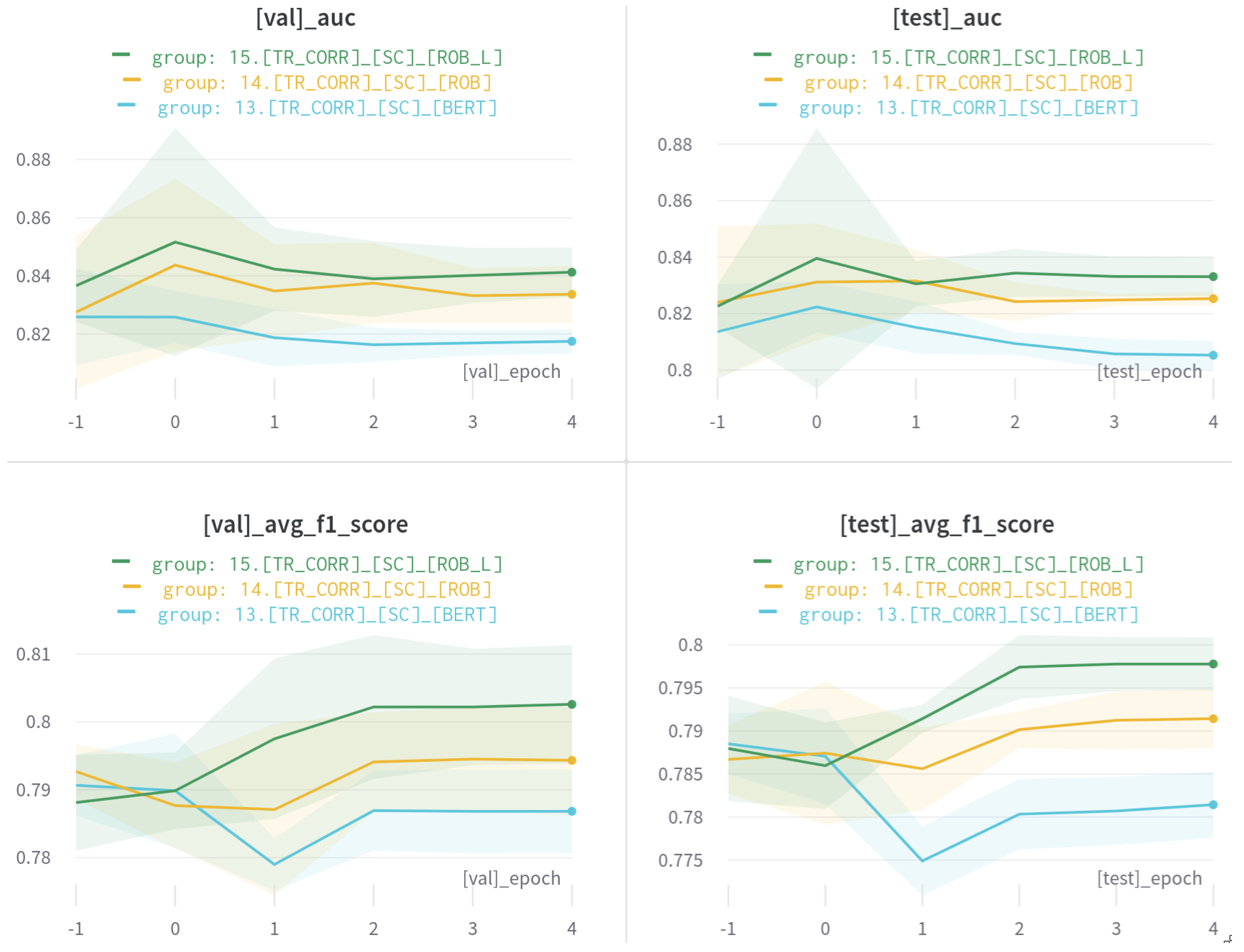
| 13.[TR_CORR]_[SC]_[BERT] | 14.[TR_CORR]_[SC]_[ROB] a | 15.[TR_CORR]_[SC]_[ROB_L] | ||||
|---|---|---|---|---|---|---|
| Val | Test | Val | Test | Val | Test | |
| Average AUC↑ | 0.8175 | 0.8053 | 0.8336 | 0.8253 | 0.8412 | 0.8331 |
| Average ↑ | 0.7868 | 0.7978 | 0.7943 | 0.7914 | 0.8026 | 0.7814 |
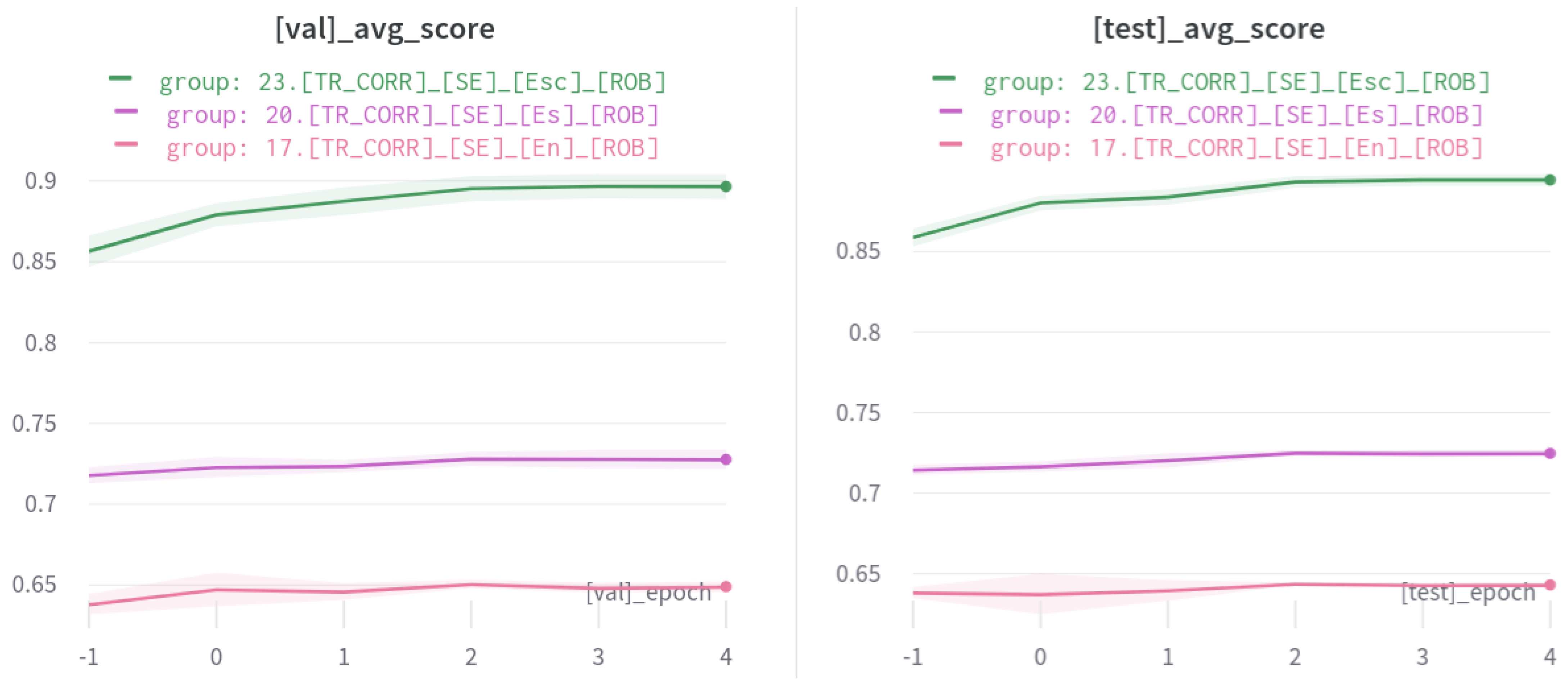
| Model | Val. Jaccard | Test Jaccard |
|---|---|---|
| 17.[TR_CORR]_[SE]_[En]_[ROB] | 0.649 | 0.643 |
| 20.[TR_CORR]_[SE]_[Es]_[ROB] | 0.7277 | 0.7247 |
| 23.[TR_CORR]_[SE]_[Esc]_[ROB] | 0.8965 | 0.8944 |
| Source of Sentiment | With Coverage | W/O Coverage |
|---|---|---|
| Classifier prediction | 0.6401 | 0.6392 |
| Manual label | 0.7265 | 0.7256 |
Publisher’s Note: MDPI stays neutral with regard to jurisdictional claims in published maps and institutional affiliations. |
© 2021 by the authors. Licensee MDPI, Basel, Switzerland. This article is an open access article distributed under the terms and conditions of the Creative Commons Attribution (CC BY) license (https://creativecommons.org/licenses/by/4.0/).
Share and Cite
Lim, J.; Sa, I.; Ahn, H.S.; Gasteiger, N.; Lee, S.J.; MacDonald, B. Subsentence Extraction from Text Using Coverage-Based Deep Learning Language Models. Sensors 2021, 21, 2712. https://doi.org/10.3390/s21082712
Lim J, Sa I, Ahn HS, Gasteiger N, Lee SJ, MacDonald B. Subsentence Extraction from Text Using Coverage-Based Deep Learning Language Models. Sensors. 2021; 21(8):2712. https://doi.org/10.3390/s21082712
Chicago/Turabian StyleLim, JongYoon, Inkyu Sa, Ho Seok Ahn, Norina Gasteiger, Sanghyub John Lee, and Bruce MacDonald. 2021. "Subsentence Extraction from Text Using Coverage-Based Deep Learning Language Models" Sensors 21, no. 8: 2712. https://doi.org/10.3390/s21082712
APA StyleLim, J., Sa, I., Ahn, H. S., Gasteiger, N., Lee, S. J., & MacDonald, B. (2021). Subsentence Extraction from Text Using Coverage-Based Deep Learning Language Models. Sensors, 21(8), 2712. https://doi.org/10.3390/s21082712