A Comparative Analysis of Signal Decomposition Techniques for Structural Health Monitoring on an Experimental Benchmark

Abstract

Signal Processing is, arguably, the fundamental enabling technology for vibration-based Structural Health Monitoring (SHM), which includes damage detection and more advanced tasks. However, the investigation of real-life vibration measurements is quite compelling. For a better understanding of its dynamic behaviour, a multi-degree-of-freedom system should be efficiently decomposed into its independent components. However, the target structure may be affected by (damage-related or not) nonlinearities, which appear as noise-like distortions in its vibrational response. This response can be nonstationary as well and thus requires a time-frequency analysis. Adaptive mode decomposition methods are the most apt strategy under these circumstances. Here, a shortlist of three well-established algorithms has been selected for an in-depth analysis. These signal decomposition approaches—namely, the Empirical Mode Decomposition (EMD), the Hilbert Vibration Decomposition (HVD), and the Variational Mode Decomposition (VMD)—are deemed to be the most representative ones because of their extensive use and favourable reception from the research community. The main aspects and properties of these data-adaptive methods, as well as their advantages, limitations, and drawbacks, are discussed and compared. Then, the potentialities of the three algorithms are assessed firstly on a numerical case study and then on a well-known experimental benchmark, including nonlinear cases and nonstationary signals.

1. Introduction

Real-life signals from vibrating structures are difficult to investigate, mainly due to the presence of measurement noise, their nonstationarity, and the noise-like distortions induced by the presence of structural nonlinearities [1]. Nevertheless, the dynamic response of a target system can disclose its mechanical properties—that is to say, its stiffness and/or mass [2]. This is also known as (linear or nonlinear) System Identification (SI/NLSI). For unchanged operational, environmental, and boundary conditions (i.e., in absence of confounding influences), the variations of these properties can be directly related to the development of damage [2]. Therefore, with a proper comparison between the current situation and the known “normal” baseline model of the system, vibration-based damage detection and Structural Health Monitoring (SHM) can be performed.

In this sense, the purpose of any decomposition technique is to isolate and extrapolate a Defect Signal Mode (DSM) from the wide-band recordings of the structural response. Then these DSMs can be used on their own or (most commonly) further post-processed individually to extract one or more Damage-Sensitive Features (DSFs) from each mode. Then, surrogate models can be defined from the DSMs and/or the DSFs collected during the structure normal conditions (the best practice would be to include data recorded during varying environmental and operational conditions to make a robust model, less subject to false alarms). This is generally performed through pattern recognition and Artificial Intelligence (AI) approaches (techniques based on Bayesian Machine Learning are particularly well-suited [1]). Finally, basic outlier detection statistical tools can be applied to discover damage-related anomalies.

The basic idea behind signal decomposition is to “break down” a complicated signal into simpler, yet similar, components, possibly rapidly and efficiently. These components—or modes—should be as independent from each other as possible, not too differently from the eigenmodes obtainable from the modal analysis of a time-independent, linear system. Eventually, they should preferably have some sparsity properties—e.g., being bandwidth limited in the frequency domain and compact around a centre frequency. A requisite is that the combination of all these components can return the original signal ideally without losses of the carried information (i.e., with minimum least-square error). All these requisites make these modes similar, but not necessarily identical, to the linear normal modes (LNMs), and the concepts should not be confused [3].

Then, these “modes” can be exploited in several manners. For instance, very low- or very high-frequency content, unrelated to the actual mechanical properties of the investigated structure, can be discarded. These tasks are referred to as denoising and baseline drift removal; both procedures are widely popular for SHM, even if one should use particular care since the removal of nonstationary components can lead to missing data information, especially for civil engineering applications when the input excitation is a ground motion [4]. Other uninteresting modes, irresponsive to damage and/or governed by other external factors (such as temperature, seasonal changes, and vibrations induced by operating machinery, pedestrians, or vehicles) can be removed as well. Nonstationary components can also be dismissed, trying to highlight time-independent mechanisms or features [5]. Finally, some modes can be found to be more sensitive to damage than others; thus, it is easier to detect small changes (e.g., due to crack development in its earlier stages) in a single component rather than in the complete signal, as these small variations may be masked by the other damage-insensitive information.

Adaptive Mode Decomposition Methods

Several algorithms have been proposed in recent years for the purposes highlighted above. A quite complete and up-to-date review can be found in Ref. [6] specifically for fault diagnosis and condition monitoring. However, at the current state, no methodical analysis has been performed on these approaches from an SHM point of view. Many review papers only enlist the applications found in the literature, reporting the findings and statements of other researchers. Other review papers perform some limited testing, generally applying the algorithms on one or few (often synthetic) signals, and with minimal commentary. The purpose of this direct comparison is to address the accuracy and efficiency of such methods for the extraction of DSFs and the subsequent Machine Learning training. Among the many proposals found in the scientific literature, the most well-known approaches include the Empirical Mode Decomposition (EMD, [7]), the Local Mean Decomposition (LMD, [8]), the Local Characteristic scale Decomposition (LCD, [9]), the Hilbert Vibration Decomposition (HVD, [10]), the Empirical Wavelet Transform (EWT, [11]), and the Variational Mode Decomposition (VMD, [12]).

All of them are more or less empirically based or retain some theoretical principles that justify the way they operate. Their common goal is to allow data-adaptive time-frequency analysis for nonstationary time histories (THs) of linear or nonlinear systems.

Of the six approaches mentioned above, the LCD follows the same framework as the EMD, with the only relevant difference lying in the instantaneous mean extraction [6]. However, this step as well uses an approach similar to the EMD, based on cubic spline interpolation, with all the same technical issues.

Similarly, the LMD as well suffers the same shortcomings as the EMD (which will be discussed later). Moreover, it has been proved to be significantly affected by the choice of the smoothing and step size parameters [6]. For all these reasons, LCD and LMD have not been considered in this comparative analysis. On the other hand, the EWT algorithm has been tested on the same numerical and experimental datasets presented in this paper. However, the specific findings are deferred to a future similar work, focused specifically on wavelet-based (adaptive or not) techniques. Due to the authors’ intent to analyse and compare the techniques in depth, some other interesting approaches e.g., the Intrinsic Time-scale Decomposition (ITD, [13]), had to be omitted because of space limitations; these will be addressed in future works as well.

Hence, the authors have selected a shortlist of three algorithms, which have reached undisputable popularity in many engineering fields and differ substantially from each other. These are the EMD, the HVD, and the VMD. All of them have been successfully applied for fault and damage detection (see e.g., References [14,15]). These three methods are here quantitatively compared. Firstly, a dataset of numerically simulated vibration is utilised to estimate the robustness to artificially added measurement noise. Then, a well-known, well-documented case study—a three-storey frame model developed at the Los Alamos National Laboratory [16]—is used as a benchmark. This simple yet compelling case study includes nonlinear distortions, stiffness reductions, and added masses. Please note that the algorithms reviewed here are neither limited to time series nor one-dimensional or single-channel data analysis; however, only this case will be addressed here, even when the respective bivariate or multivariate extensions exist (e.g., [17,18]).

The rest of this paper is organised as follows. The theory and mathematical formulation behind the three alternatives investigated here are reported in Section 2. The advantages and limitations of each approach are recalled as well. Section 3 describes the experimental benchmark utilised for this comparative study, as well as the parameters selected for this aim. Section 4 discusses the results. This work ends with the conclusions.

2. Theoretical Background

In this section, the theory behind the three decomposing techniques of interest is addressed. As recalled, all these approaches break down the target signal into various components. This can be performed directly in the time domain (such as for the EMD and derived techniques), in the frequency domain (e.g., the VMD), or in the time-frequency (or time-scale) plane. The rationale behind frequency- and time-frequency-based decomposition techniques is that most real-world signals have compact, band-limited Fourier spectra; methods of this kind implicitly assume that the independent components of the signal have narrow-band properties and (generally) well-distinct spectrum supports [19]. What differentiates the approaches here reviewed from the classic Fourier transform (FT) is that they all allow the investigation of time-varying (nonstationary) signals. The techniques are analytically or empirically defined, i.e., they operate according to an algorithm but lack a proper mathematical definition. That provides them with some degrees of data adaptability.

The three methodologies are described in detail in the following subsections. The discussion starts with the EMD (and subsequent variants), the HVD, and the VMD, in this order. Since the estimation of the instantaneous frequencies (IFs) and amplitudes (IAs) is necessary for the analysis of the resulting modes, the definition of the Hilbert transform (HT) is recalled in the subsection dedicated to the EMD.

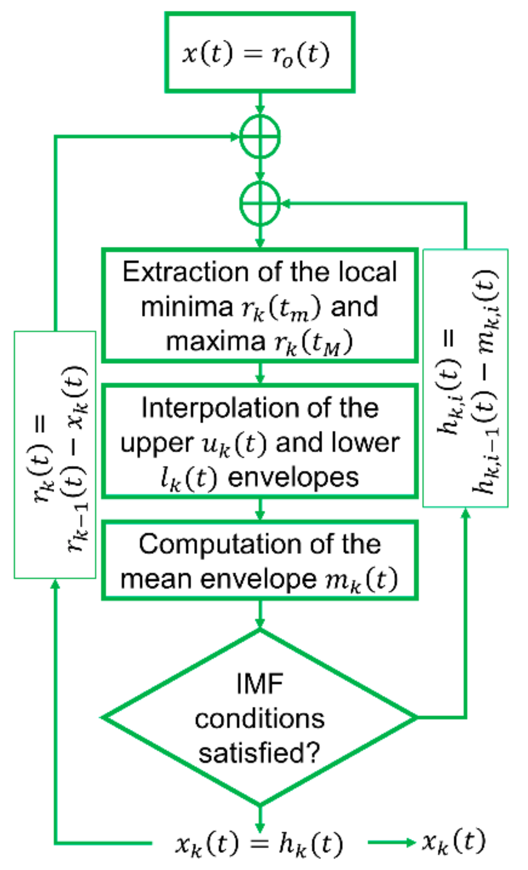
2.1. Empirical Mode Decomposition (EMD) and Derived Algorithms

Since its first introduction in 1998 [7], the Empirical Mode Decomposition (EMD) has been widely studied and applied in many fields. For structural purposes, it has been exploited for System Identification (e.g., [20,21]), also by approximating the eigenmodes of bridges for Operational (i.e., output-only) Modal Analysis [22], even during extreme events [23]. It has been applied for the SHM of steel frame structures [24] as well, among many other similar applications. The technique is particularly appreciated for the condition monitoring of rotating machinery (see Ref. [25] for a dedicated overview). Some other useful reviews for SHM purposes can be found in [26], in the very recent Ref. [14], and in Chapter 14 and 15 of Ref. [27].

The EMD is used to decompose the target signal into a finite (and generally small) number of natural oscillatory modes, which are called IMFs (Intrinsic Mode Functions) [7]. The IMFs are oscillations incorporated in the original signal, and their amplitude and frequency are not constant over time, unlike the harmonics that are obtained with the Fourier transform [28]. That is to say, the IMFs preserve their instantaneous frequency information.

With the Hilbert Spectral Analysis (HSA), the EMD forms the basis of the Hilbert–Huang Transform (HHT) for the estimation of the IFs and of the time-frequency distribution of the signal amplitude (i.e., the Hilbert–Huang Spectrum $H\left(\omega ,t\right)$). If the HSA was performed directly on the whole (non-decomposed) signal, it could return physically impossible results such as negative frequencies [28]. Instead, the use of IMFs enforces physically meaningful results. This is achieved by imposing some rules on how an IMF is defined. Specifically, for a function to be considered an Intrinsic Mode Function, it must satisfy the following two conditions:

• The number of local maxima and minima and the number of points where it assumes a zero value must be equal or at most differ by one unit;
• The local mean, defined as the mean of the upper hand lower envelopes, must be zero.

Thus, the IMFs are essentially zero-mean AM-FM components. Then, the original signal can be reconstructed directly as the sum of all IMFs in the time-domain [7]. Importantly, the IMFs have no analytical formulation [29]. This is related to the EMD being an algorithm, i.e., a set of arbitrary (and empirical, as the name suggests) rules that can be applied to a dataset and lack a well-defined theoretical basis (differently from, e.g., the FT). The EMD decomposition procedure, also known as the “sifting process” [30], is described in details in Ref. [7]. The complete description is omitted here for brevity; a graphical depiction is portrayed in Figure 1, where, at any $k$-th step, the sifted signal (i.e., the residual) is called $r_k\left(t\right)$ (for $k=0$, $r_{k=0}\left(t\right)=x\left(t\right)$). The average between the upper and lower envelopes returns $m_k\left(t\right)$, and the difference $r_k\left(t\right)-m\left(t\right)$ is iterated over the additional counter $i$ until it satisfies the two conditions by which an IMF is defined. At that point, $x_k\left(t\right)$ is the $k$-th IMF and the new residual is calculated. The algorithm stops when the $K$-th residual $r_K\left(t\right)$ is a monotone function or a function with less than two local minimum or maximum points.

A major technical limitation of the basic EMD definition is the issue of the so-called “mode-mixing” when the method is applied to signals affected by measurement noise (or noise-like nonlinear disturbances). This phenomenon involves the over-decomposition of a signal, and it leads the algorithm to extract more IMFs than the number of oscillatory modes that make up the original signal. The mode-mixing is due to EMD being a completely data-driven technique: the addition of noise involves the creation of “fictitious” maximum and minimum points that are identified by the algorithm and interpolated. This causes even a mono-component signal such as a simple sinusoid to be broken down into several sub-signals when affected by noise [31]. This high sensitivity to noise limits the reliability of an EMD-based signal monitoring scheme. However, to alleviate the mode mixing problem, a series of improvements have been introduced, representing the direct evolution of the EMD algorithm:

• The Ensemble Empirical Mode Decomposition (EEMD; [31]);
• The Complete Ensemble Empirical Mode Decomposition with Adaptive Noise (CEEMDAN; [32]).

These two improvements to the basic EMD can be found in the respective references. Here, in this study, the CEEMDAN algorithm was applied to the benchmark dataset of interest. This involves the use of $N_R$ realisations of White Gaussian Noise (WGN) defined by the noise standard deviation $ϵ$. This improved variant is supposed to strongly reduce the detrimental effects of noise, even if at the cost of being more computationally intensive.

The Hilbert Transform

Once all the IMFs have been defined, the Hilbert transform [7] can be applied to them as:

$$y_k\left(t\right)=\frac{1}{\pi }\mathrm{p}.\mathrm{v}.{{\displaystyle \int }}_{-\infty }^{\infty }\frac{x_k\left(\tau \right)}{t-\tau }d\tau$$

(1)

where $\mathrm{p}.\mathrm{v}.$ denotes the Cauchy principal value. Equation (1) can be considered as the convolution of the k-th mode with $1/t$, which is intended to emphasise the instantaneous properties of $x_k\left(t\right)$. To define their time-varying IF and envelope of the signal, it is then sufficient to compute

$${\omega }_k\left(t\right)=\frac{d\phi \left(t\right)}{dt}$$

(2)

where $\phi \left(t\right)=\arctan \frac{y\left(t\right)}{x\left(t\right)}$ is the instantaneous phase, and

$$A_k\left(t\right)=\sqrt[2]{x_k^2\left(t\right)+y_k^2\left(t\right)}.$$

(3)

is the IA. For all the other details concerning the HT, the interested audience is referred to the extensive tutorial review presented in Ref. [33].

Please note that several other techniques are available for the estimation of instantaneous parameters. Indeed, the HT has some well-known flaws—it is limited by the Bedrosian theory, can return negative instantaneous frequencies, and suffers from energy leakage at the signal edges, making the estimation of the IF and IA unreliable close to them [34]. The HT is also very sensitive to noisy data since it requires the derivative of both the real and the imaginary part of the transformation [35]. The same issues affect similar procedures such as the Wigner–Ville Distribution (see Ref. [36] for a more detailed discussion). A much better estimation of the IF can be achieved e.g., by simply considering the time sequence of the signal zero-crossing points [35,37].

The potential alternatives include the Energy Separation (ES, [38]), the Teager Energy Operator (TEO) [39], the Normalised Hilbert Transform (NHT), the Generalised Zero Crossing (GZC), and the Direct Quadrature (DQ) algorithms (the last three are all presented in Ref. [34]), plus other options derived from them, e.g., the Quadrature Derivative based Normalised HT (QDNHT, [40]). These approaches, among many others, have been proposed to address some of the HT shortcomings. However, this point does not fall into the specific aim of this study and it will not be further discussed for brevity; a detailed comparison can be found e.g., in Ref. [6].

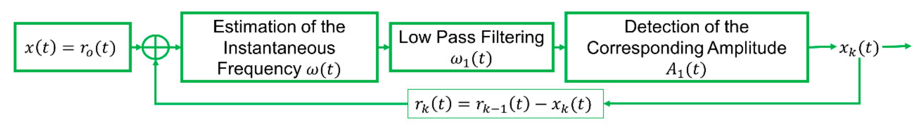
2.2. Hilbert Vibration Decomposition (HVD)

The Hilbert Vibration Decomposition (HVD) was introduced by Feldman in 2006 [10] for the extraction of components (modes) from nonstationary broadband signals. The method is similar to EMD (and derived techniques) in the sense that it is still a recursive decomposition scheme performed iteratively on the residual signal from the previous step [12]. The HVD approach relies on the Hilbert transform (HT), as the name suggests. The interested reader is referred to Feldman’s book [41] for a deeper discussion. At any iteration, the dominant (i.e., most energetic) vibration is extracted; its IF is estimated as the average frequency obtained from the HT. This is intended to enforce that any inherent component has mathematical and physical significance, rather than merely satisfying some user-defined requisites [10].

The HVD method has been proposed for SHM applications [42], even if its main field of application remains the SI of nonlinear mechanical systems [43]. The HVD algorithm has been validated on nonlinear systems with single or multiple degrees of freedom (e.g., in Ref. [44] for a two-DoF system), even if not yet on large real-life structures [45].

The basic assumption is that the original signal is formed by a superposition of harmonic or quasi-harmonic functions. If the signal is multi-component, then it can be decomposed into several, distinct mono components [46]; for continuous time, this operation can be intended as

$$f\left(t\right)={\displaystyle \sum }_{k=1}^K{x}_k\left(t\right)={\displaystyle \sum }_{k=1}^K{A}_k\left(t\right)\cos \left(\int {\omega }_k\left(t\right)dt\right)$$

(4)

where $f\left(t\right)$ is the whole signal and $x_k$ are its single-mode terms defined by their instantaneous amplitudes and frequencies ($A_k\left(t\right)$ and ${\omega }_k\left(t\right)$, respectively). Then, the instantaneous phase of the signal is given by ${\phi }_k\left(t\right)=\int {\omega }_k\left(t\right)dt$. Importantly, the authors of the EMD algorithm did not provide a similar analytical definition for their IMFs. Every $x_k\left(t\right)$ is assumed to be a simple waveform, with slowly varying $A_k\left(t\right)$ and ${\omega }_k\left(t\right)$. This assumption has important repercussions on the properties of the extracted modes; these will be better addressed later. The HVD iterative algorithm can be summarised in three sequential steps. Specifically:

• The instantaneous frequency of the vibration component with the largest energy content (i.e., amplitude) is estimated;
• The envelope of the same is extracted;
• The component is subtracted from the signal.

Then, the residual is passed to the next iteration until the desired number K of modes is extracted. A block diagram description of the algorithm is reported in Figure 2. One can see that a major conceptual difference between EMD and HVD is that the former algorithm independently estimates IF (via zero-crossing) and IA, while the latter only estimates the IF and then extracts the corresponding IA. This choice has both advantages (such as a better frequency resolution) and disadvantages [47].

A more complete and detailed description of the whole algorithm can be found in the original work of Feldman [10]. Figure 3 reports an example of an application of the HVD technique to an experimental dataset. $K=2$ was imposed. The signal, a displacement TH, comes from a cantilevered aluminium box beam, with two saw-cuts intended to mimic surface open cracks and subject to 11-$\mathsf{\mu }\mathrm{s}$-long triangular impulses. The full description of the setup can be found in Ref. [48]. In this example, the first IMF can be linked to the steady-state free oscillation of the beam, while the second one captures the transient effects of the input, similarly to what expected for the forced nonstationary response of the inspected system [10]. However, far from the input, the transient term fades away. By increasing $K$, no other relevant IMF arises, hinting at a single-component linear behaviour (as expected for this specific structure, which behaved linearly even after damage insertion).

2.3. Variational Mode Decomposition (VMD)

Even if not yet as widespread as EMD, the VMD algorithm (proposed in 2014 by Dragomiretskiy and Zosso [12]) has been already extensively applied in Structural Engineering. Ref. [49] applied it for the SI of time-dependent systems, such as a bridge with a passing vehicle (simulated on a laboratory experiment). Ref. [50] validated it for the output-only approximation of the vibrational modes of a pedestrian bridge, proposing the approach for SHM uses as well. Ref. [51] applied the VMD for the fault detection on rotating machinery and for NLSI, showing how VMD returned separate modes corresponding to the frequency of the driving force, the first superharmonic (2×), and the most pronounced subharmonic (1/3×), plus the higher-frequency content.

The VMD assumes the definition of “modes” introduced by the HVD [10] i.e., as seen before, amplitude-modulated–frequency-modulated (AM–FM) sub-parts of the whole signal, which can be reconstructed by simply summing them up in the time domain. By recalling Equation (4), these modes must satisfy the following conditions: (1) the envelope must be non-negative ($A_k\left(t\right)\ge 0 \forall t$); (2) the phase must be non-decreasing—i.e., it must have a non-negative first-time derivative ($\phi {\prime }_k\left(t\right)\ge 0 \forall t$); (3) both the instantaneous amplitude $A_k$ and the instantaneous frequency ${\omega }_k$ must vary much slower than the instantaneous phase ${\phi }_k$. This concept is shared not only by the HVD but also by e.g., the synchrosqueezed wavelet transform and by the EWT, among many other similar approaches. The rationale for this additional requirement is that for an interval $\left[t,t+∆t\right]$ long enough (i.e., with $∆t$ at least circa equal to $2·\left(\frac{2\pi }{{\omega }_k}\right)$), the k-th IMF can be approximated to a pure harmonic function with time-varying (instantaneous) amplitude $A_k\left(t\right)$ and frequency ${\omega }_k=\phi {\prime }_k\left(t\right)$. This is quite different from the classic EMD definition of IMF, where the modes’ supports may span over a large range of frequencies with more peaks. Since all the original IMF requirements are still met, this alternative definition can be seen as a restriction of EMD’s IMFs [12]. The outcome is a limited (in practical terms) bandwidth IMF, which is compact around a centre frequency. Please note that the spectral support of an FM signal is theoretically infinite; yet, the core of the signal’s power content may be bounded according to Carson’s rule [52], which can be here used to define the total IMF bandwidth (with a correction accounting for the frequency of the amplitude modulation) [12]. For this reason, the modes defined as in Equation (4) are also known as Band-Limited Intrinsic Mode Functions (BLIMFs). The signal (and therefore its constituent modes) is also required to be integrable and square-integrable up to second derivatives [12]. Then, the IFs of time-dependent modes can be estimated employing the HT on the extracted BLIMFs, not differently from the EMD and derived approaches.

The basic scheme of the VMD algorithm is recalled here; a more detailed description of the complete algorithm can be found in the original work [12]. In brief:

• For each mode $x_k\left(t\right)$, the associated analytic signal is computed employing the Hilbert transform. The result is a unilateral frequency spectrum (the negative frequencies of the FT spectrum are discarded, as they do not have physical meaning and are superfluous due to the Hermitian symmetry);
• Each mode’s spectrum is re-centred on the estimated centre (angular) frequency ${\omega }_k$ by mixing with a tuned exponential function;
• The bandwidth is eventually estimated through the $H^1$ Gaussian smoothness of the demodulated signal, which is the squared Euclidean norm ($L^2$-norm) of the gradient.

These three steps translate into a constrained variational problem, the complete analytical explanation of which can be found in the original work of Dragomiretskiy and Zosso [12]. Importantly, the number K of modes to be extracted is chosen a priori by the user (as for the HVD).

2.4. Qualitative Comparison of the Techniques

The main characteristics of the three algorithms are summarised in

Table 1. Main features of the described methods.

Feature	EMD	HVD	VMD
Basis	Self-Adaptation	Self-Adaptation	Prior Determination
Frequency	Difference, Local	Difference, Global	Difference, Global
Characterisation domain	Energy-Time	Energy-Time-Frequency	Energy-Time-Frequency
Apt for nonlinear systems?	Yes	Yes	Yes
Apt for nonstationary signals?	Yes	Yes	No
Feature extraction	Yes	Yes	Yes
Theoretical foundations	Empirical	Complete Theory	Complete Theory

. The EMD, being empirical by definition, operates within an “algorithmic ad-hoc nature” [12] and lacks any physical justification and a a proper mathematical definition (both of the algorithm and the extracted IMFs). The other two techniques are more defined from an analytical point of view. VMD and HVD share the same requisites for band-limited IMFs, which are slightly different (and stricter) from the original IMF definition adopted for the EMD. The additional requirement of slowly time-changing properties limits the applicability of the methods; however, they still cover many real-life scenarios. On the other hand, the BLIMF definition better enforces quasi-orthogonal signal decomposition [51].

The EMD/EEMD/CEEMDAN algorithms return a fixed number of IMFs (based on the time-varying properties of the time series). The HVD and VMD require the user to pre-define the number K of modes to be extracted. Both options have pros and cons. Essentially, the more a decomposing technique is data-driven, the more likely it may end up being overfitted over a single signal, making the comparison between different signals more problematic. Conversely, without some specific knowledge, it may be difficult to estimate a priori the number of independent modes.

Ref. [53] compared the VMD and EMD for the analysis of seismic signals, claiming that the former outperforms the latter. For the same application, Ref. [54] suggested using EMD and HVD combined, as the former is more reliable for high-frequency content and the latter is more reliable for high energy, low-frequency ones. Ref. [55] highlighted a larger accuracy of support-vector machines (SVM) classifiers trained on VMD-extracted BLIMFs in comparison to the ones trained with other signal components. Therefore, the VMD is expected to compare well with respect to the other options (this point was confirmed by the findings of this research, as it will be shown later).

For a deeper analysis, the full list of advantages and disadvantages of the three methods, as mentioned in the reviewed papers, is reported in the three tables of Appendix A.

3. The Numerical and Experimental Case Studies

For the sake of this comparative analysis, two datasets, one numerical and one experimental, have been used. The former case study was investigated to properly address the performances of the three techniques on ideal conditions, i.e., with noise-free vibrations. Then, the effects of artificially added WGN and sensor placement have been studied as well. All the other investigations were performed directly on the experimental data.

3.1. The Numerical Dataset

The first dataset is made up of the simulated response of the Finite Element Model (FEM) of the spar for the prototype XB-1 wing [56]. Its geometry and mechanical properties are reported in

Table 2. Geometrical and mechanical properties of the wing spar Finite Element Model (FEM).

Property	Value	Measurement Unit
Free length (clamp to tip) $l_{TIP}$	706.00	mm
Thickness $t$	2.00	mm
Max width at the Clamped section $b_{\mathrm{MAX}}$	180.00	mm
Min width at the tip section $b_{\mathrm{MIN}}$	17.04	mm
Young’s modulus	$59.02\times {10}^3$	MPa
Density	2893.07	$\mathrm{kg}/{\mathrm{m}}^3$
Damping ratio	0.86	%
Poisson’s ratio	0.26	-

. Due to the high flexibility of the structure, minimally invasive and non-contact measurements were needed to investigate the structure; specifically, the video processing procedure of Ref. [57] was applied for the FE Model Updating.

The linear FE analysis was run on ANSYS^® Mechanical APDL™ emulating the experimental setup described in Ref. [58]—i.e., clamped-free, with Inertial Measurement Units (IMUs) attached to the four points marked in Figure 4.

A random noise excitation was applied to the wingtip, perpendicularly to the spar with a peak acceleration of 1.5 g. A total of 1280 data points per output channel and simulation were collected, for a sampling frequency of 256 Hz and a duration of 5 s. The first flapwise bending mode was clearly identifiable from the noise-free signals at 5.49 Hz. To a lesser extent, the second mode at 23.16 Hz can be noticed as well. The response signals were then artificially corrupted with increasing levels of additive WGN, which were defined from 0 to 0.01 standard deviations of the original signal in steps of ${10}^{-4} \sigma$. The MatLab randn() function was utilised for this purpose.

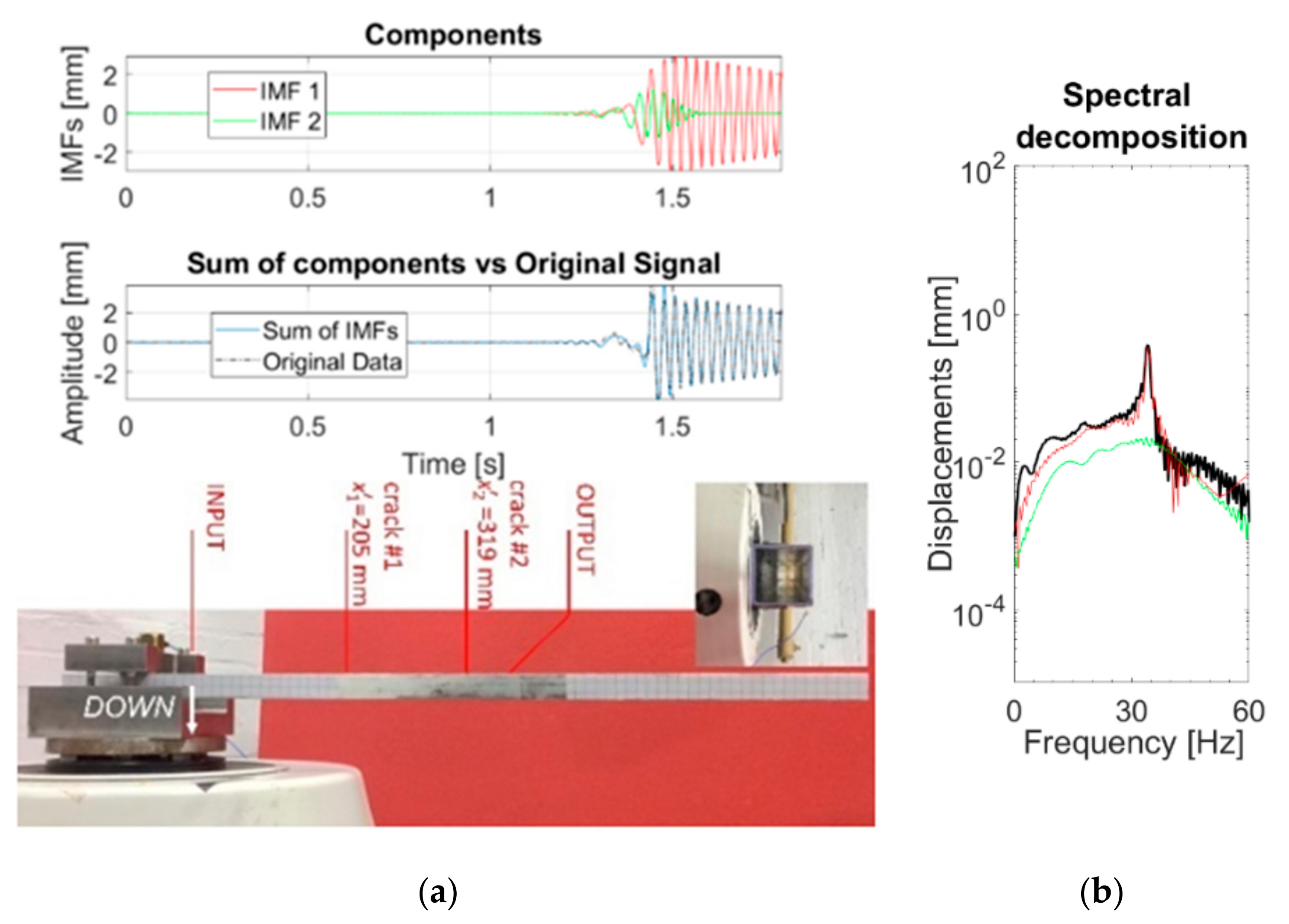
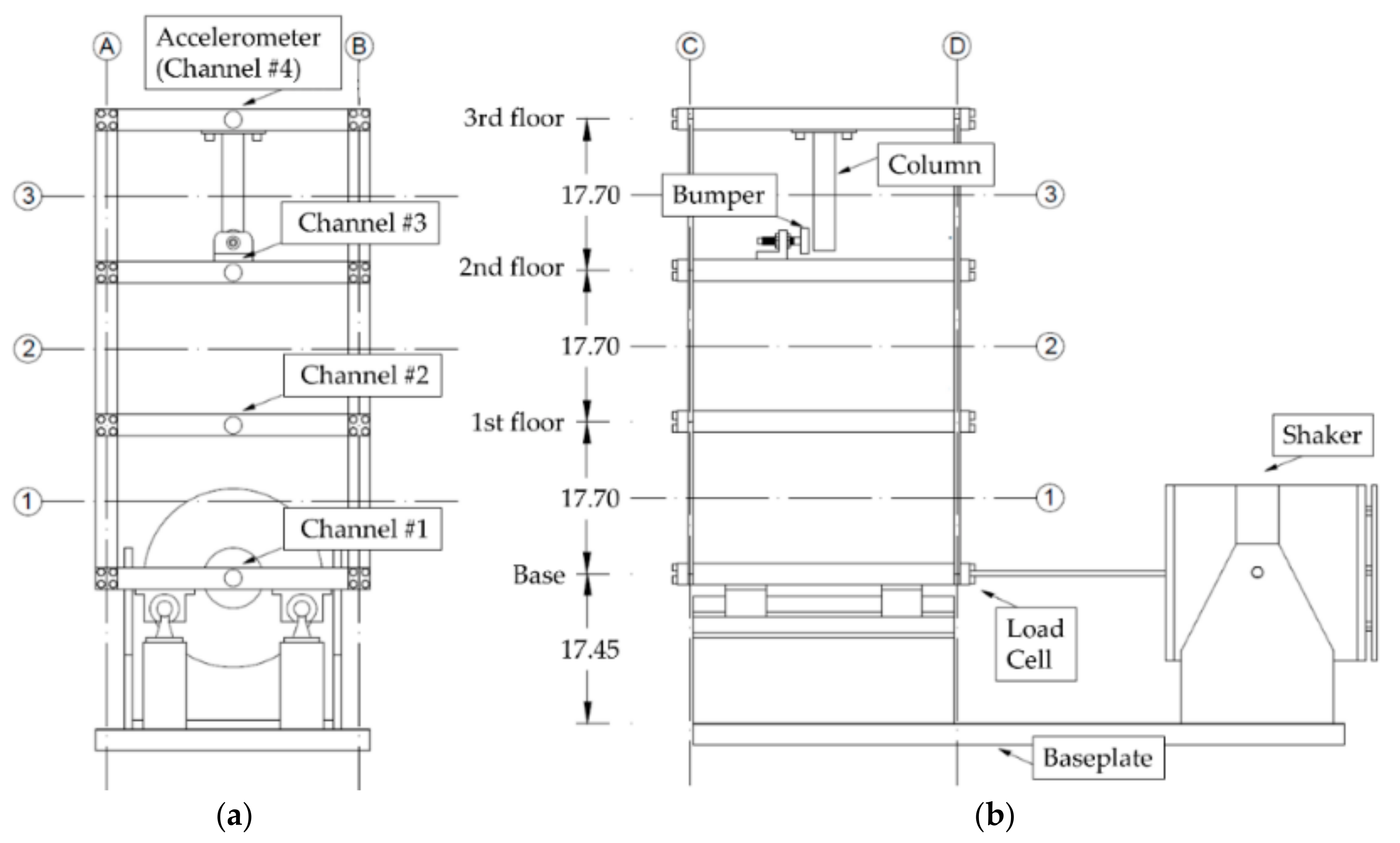
3.2. The LANL Benchmark

The comparison of the signal decomposition techniques has been mainly performed on a well-known experimental benchmark, which was proposed by the Los Alamos National Laboratory (LANL) and fully described in References [16,59]. The main points are here recalled for completeness. The test structure is a three-storey shear-type frame, excited horizontally at the moving base. A scheme of the test frame, adapted by the authors from Ref. [59], is reported in Figure 5 (the shaker and the sensors’ positions are highlighted). Please note that only one output channel per floor was available. However, this is sufficient to fully characterise the model under the assumption of shear-type frame behaviour, which is well justified here. The model presents two typical forms of detectable damage-induced features: (1) a localised reduction of the stiffness, and (2) a pointwise source of nonlinearity. It also introduces added masses to simulate damage-unrelated operational changes [59].

The clapping behaviour, intended to mimic a so-called “breathing crack”, was achieved by introducing a bumper–column bilinear mechanism. The nonlinearity of the system is governed by moving the bumper closer to the column’s tip, such that it comes in touch with the bumper at lower input amplitudes. It is important to state that in a real-life structure with breathing surface cracks, the stiffness will be equal to the one of the pristine structure on the closing direction and reduced on the opening side (see Ref. [60] for a more detailed discussion). In this setup, the stiffness is unchanged in the opening direction and augmented in the opening one. This returns a global increase of the total stiffness for the “damaged” scenarios, rather than a decrease, as one would expect. Nevertheless, this setup (1) introduces damage-induced-like nonlinear effects in the vibrational response and (2) generates frequency shifts that are detectable with outlier detection approaches.

The Experimental Campaign

The total duration of each acquisition is 25.60 s, with a sampling frequency $f_s=320$ Hz. Thus, the response signals result in an 8192-points time series; their frequency spectra consist of 3600 frequency samples, up to a maximum frequency of 140.6 Hz at a resolution of 0.0391 Hz. These sampling parameters were deemed adequate for the intended uses (being the highest natural frequency about half of the available bandwidth upper bound) [59].

The input force (a band-limited random excitation, ranging from 20 to 150 Hz) is reported in newtons, while the four output channels captured the response in terms of acceleration time histories (here reported in g, with $1 \mathrm{g}= 9.81 \mathrm{m}/{\mathrm{s}}^2$). The campaign included a baseline scenario and sixteen alterations (all reported in

Table 3. The experimental dataset.

Case	Description
1	Undamaged baseline
2	Undamaged with confounding influences; added mass of 1.2 kg at the base
3	Undamaged with confounding influences; added mass of 1.2 kg at the 1st floor
4	Linear damage; 87.5% stiffness reduction in one column of the 1st inter-storey
5	Linear damage; 87.5% stiffness reduction in two columns of the 1st inter-storey
6	Linear damage; 87.5% stiffness reduction in one column of the 2nd inter-storey
7	Linear damage; 87.5% stiffness reduction in two columns of the 2nd inter-storey
8	Linear damage; 87.5% stiffness reduction in one column of the 3rd inter-storey
9	Linear damage; 87.5% stiffness reduction in two columns of the 3rd inter-storey
10	Nonlinear damage; distance between bumper and column tip 0.20 mm
11	Nonlinear damage; distance between bumper and column tip 0.15 mm
12	Nonlinear damage; distance between bumper and column tip 0.13 mm
13	Nonlinear damage; distance between bumper and column tip 0.10 mm
14	Nonlinear damage; distance between bumper and column tip 0.05 mm
15	Nonlinear damage with confounding influences; Bumper 0.20 mm from column tip, 1.2 kg added at the base
16	Nonlinear damage with confounding influences; Bumper 0.20 mm from column tip, 1.2 kg added on the 1st floor
17	Nonlinear damage with confounding influences; Damaged bumper 0.10 mm from column tip, 1.2 kg added on the 1st floor

).

Fifty realisations per scenario were performed. For the sake of this study, the experiments are considered as follows: Case 1 is the pristine structure that serves as a baseline model; Cases 2 and 3 present damage-unrelated frequency shifts due to confounding influences (i.e., additional masses, located at different positions); Cases 4 to 9 present damage-related frequency shifts, induced by stiffness reduction with no nonlinear sources; Cases 10 to 14 are affected by damage-like nonlinearities, which mimic a breathing crack model (with all the caveats explained before). Finally, Cases 15 to 17 are affected by nonlinearities and confounding influences.

4. Results

In this section, the extracted IMFs are extracted, visualised, and commented on; their comparability is also addressed. Then, their capabilities for ML-based SHM are tested. The parameters of the CEEMDAN, HVD, and VMD algorithms were set as follows:

• For the CEEMDAN, the improved version of the code described in Ref. [30] has been utilised. This requires the following inputs:
  • The maximum number of sifting iterations allowed;
  • The number $N_R$ of WGN realisations;
  • The standard deviation $\sigma$ of the applied noise.
  Here, a noise SD of $\sigma =0.2$ was applied for $N_R=15$, with a maximum of 3000 sifting iterations. Noteworthy, the original implementation of the code uses a pseudorandom number generator to generate the WGN realisations; this may affect the replicability of the results.
• For the HVD, the original scripts released by Feldman for use with his book (Ref. [41]) have been applied. The user-defined parameters, which should be inserted manually, are:
  • The filter cut-off frequency (suggested to be in the range $0.05>f_p>0.005$);
  • The number K of modes to be extracted.
  In this study, $f_p$ was set to the recommended minimum value of $0.005$. Regarding K, this parameter was set to 3 to represent the a priori knowledge of the user (i.e., that the mechanical system can be well-approximated by a three DoF oscillator).
• For the VMD, the original code has been used (released in 2013 by the authors and downloadable at https://math.montana.edu/dzosso/code/index.html, last visited 20 October 2020). An official MatLab implementation has been made available in the Wavelet Toolbox (https://it.mathworks.com/help/wavelet/ref/vmd.html; last visited 20 October 2020) since early 2020; however, this latter version has not been tested here. The arbitrarily defined parameters, which may influence the final results, are
  • The initial values of $\left\{x_k^1\right\},\left\{{\omega }_k^1\right\},$ and ${\lambda }^1$: $\left\{x_k^1\right\}$ and ${\lambda }^1$, which are generally all assumed as zeros at the first iteration, while the frequencies in $\left\{{\omega }_k^1\right\}$ can be initially zeroed, uniformly distributed, or random;
  • α, the balancing parameter that defines the data-fidelity constraint;
  • τ, the time-step of the dual ascent that determines the updating of the Lagrangian multipliers (generally defined to have an exact reconstruction or to achieve denoising);
  • $ϵ$, the tolerance of the stopping criterion (generally around ${10}^{-6}$);
  • The number K of modes to be extracted.

The algorithm can be also used to remove the DC offset of the input signal if needed. In this study, the following conditions were considered: $\mathsf{\alpha }=2000$ (moderate bandwidth constrain), $\mathsf{\tau }=0$ (no strict fidelity enforcement), no DC offset correction, a uniform initial distribution of the $\left\{{\omega }_k^1\right\}$, and $ϵ={10}^{-7}$. The number K was set to 3 as explained before for the HVD for comparability.

Only for descriptive purposes, the cases portrayed here in the figures of this section refer to the response to the 25th realisation unless otherwise stated. All the 50 driving forces had similar amplitude and Power Spectral Density and led to comparable results. For conciseness, only the IMFs extracted from output channel #4 (i.e., at the highest floor) and for the first case (undamaged, linear baseline) are described in detail.

In the respective subsections, these are compared to the results from the fourteenth scenario (i.e., the most nonlinear case, with no added mass or reduced stiffness) to visualise how the algorithms compare with and without nonlinear distortions and to the other (linear and nonlinear) cases to address the effects of the structural changes. To take into account the input frequency range (20–150 Hz), all the algorithms were tested on the unfiltered, low-pass filtered, high-pass filtered, and band-pass filtered signals. All figures refer to the original (unfiltered) signals if not otherwise indicated. For interpretation of the references to colour in the figure legends, the reader is referred to the online version of this article.

4.1. Preliminary Results for Noise Sensitivity and Sensor Placement

Before being compared on the experimental dataset, the selected techniques have been tested on a numerical dataset for their robustness to artificially added measurement noise and their sensitivity to sensor placement.

For simplicity, the HVD and VMD algorithms were set to return only the first IMF; in both cases, this mode was basically corresponding to the first natural frequency. For comparability, the mode most similar mode (frequency-wise) was selected from the ones returned by the CEEMDAN algorithm. In almost all simulations, this was the 4th CEEMDAN IMF. The frequency corresponding to the peak amplitude of the identified IMF (hereinafter, the peak frequency $f_p$) was used as the feature of interest. This feature was expected to remain unvaried for unchanging structural conditions. Therefore, an arbitrary threshold was set to $\pm 10\%f_p$ and considered as the maximum error allowed.

Figure 6 compares the selected IMF for CEEMDAN, HVD, and VMD for the four output channels depicted in Figure 4 and the noise-free scenario. One can observe that for this specific case, the identification of the selected mode was consistently centred around the fundamental frequency of the HAR wing spar, with negligible differences due to the specific sensor location.

As the noise level increases, the signal becomes more and more similar to a pure WGN (see Figure 7). This makes the identification procedure much more compelling. Figure 8 reports the peak frequency for increasing noise level (added according to what is specified in Section 3.1). In this case, the differences between the three techniques and the four channels are evident. As expected for the first flexural mode of a cantilevered beam-like structure, the recordings closer to the free tip (IMU #3) returned the identifications most robust to the additive noise in all cases.

For the CEEMDAN algorithm, the identifications from IMU #3 always fell in the range considered as acceptable, while the other sensors started to exceed the maximum threshold between $0.002 \sigma$ and $0.006 \sigma$, depending on their distance from the clamped end.

For the HVD method, the values of the other IMUs started to increase from $0.001\sigma$ and rapidly escalated.

The VMD method returned the most robust identifications. Not only IMU #4 but also IMU #3 were stable or almost stable for all noise levels. The remaining two channels only started to diverge significantly after $0.065\sigma$, and the absolute error was never larger than 1 Hz.

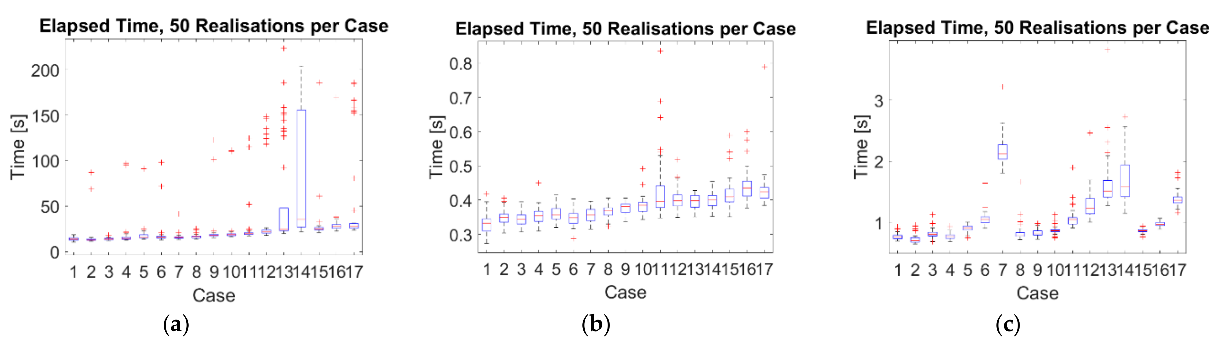
4.2. Computational Time Required

The computational times elapsed for running the non-optimised scripts on MatLab R2018b are discussed here, considering the experimental dataset.

All the runs were performed on an Intel^® Core™ i7-7700HQ CPU with a 2.80 GHz base frequency. The data pre- and post-processing phases have been excluded, focusing exclusively on the decomposition algorithms. The results, which refer to channel #4 and are averaged over 50 realisations per case, are compared in Figure 9.

The candidate algorithms compared quite differently. The HVD, being by far the simplest algorithm, run almost 2.3 times faster than VMD and circa 40 times faster than CEEMDAN for the linear baseline. The CEEMDAN algorithm showed the largest variability due to its step involving the addition of random WGN. As expected, for all three options, the cases with the added nonlinearity were the ones most computationally demanding. The VMD encountered major difficulties in dealing with case #7 as well.

Even if this study focusses on offline data interpretation, these results are also important in consideration of potential applications for real-time damage detection and online modal identification, which require minimal computational expenses [61].

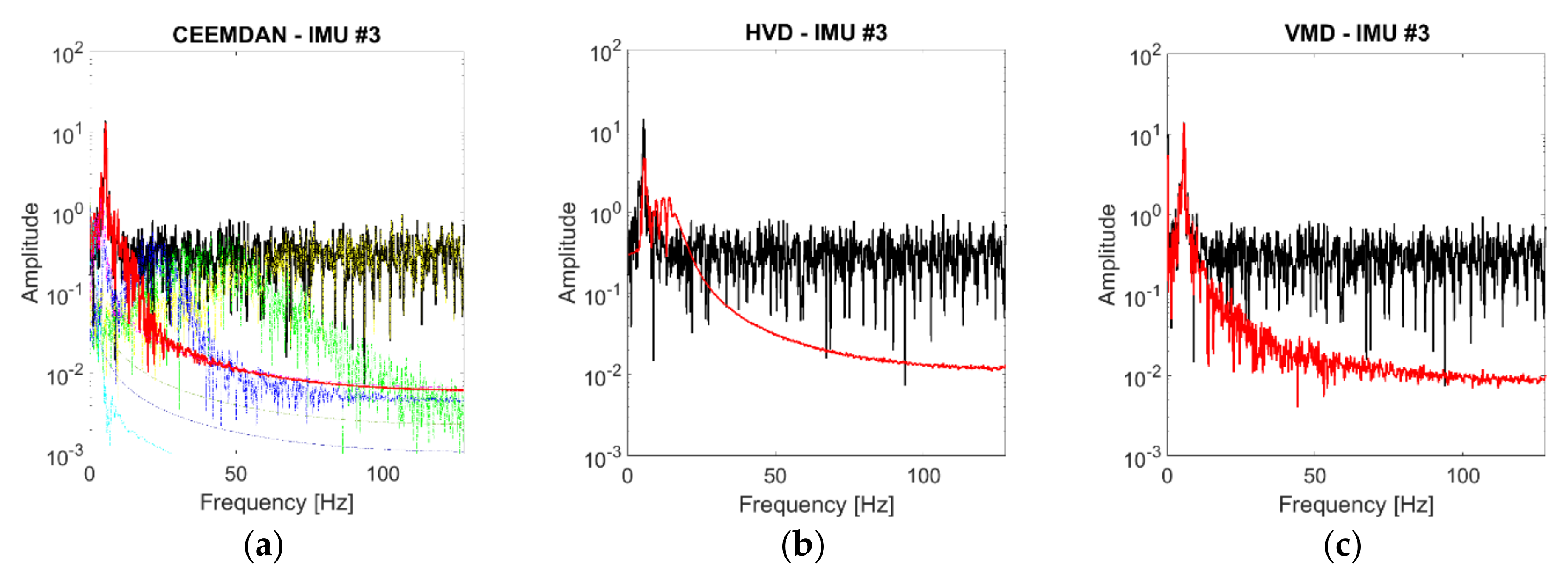
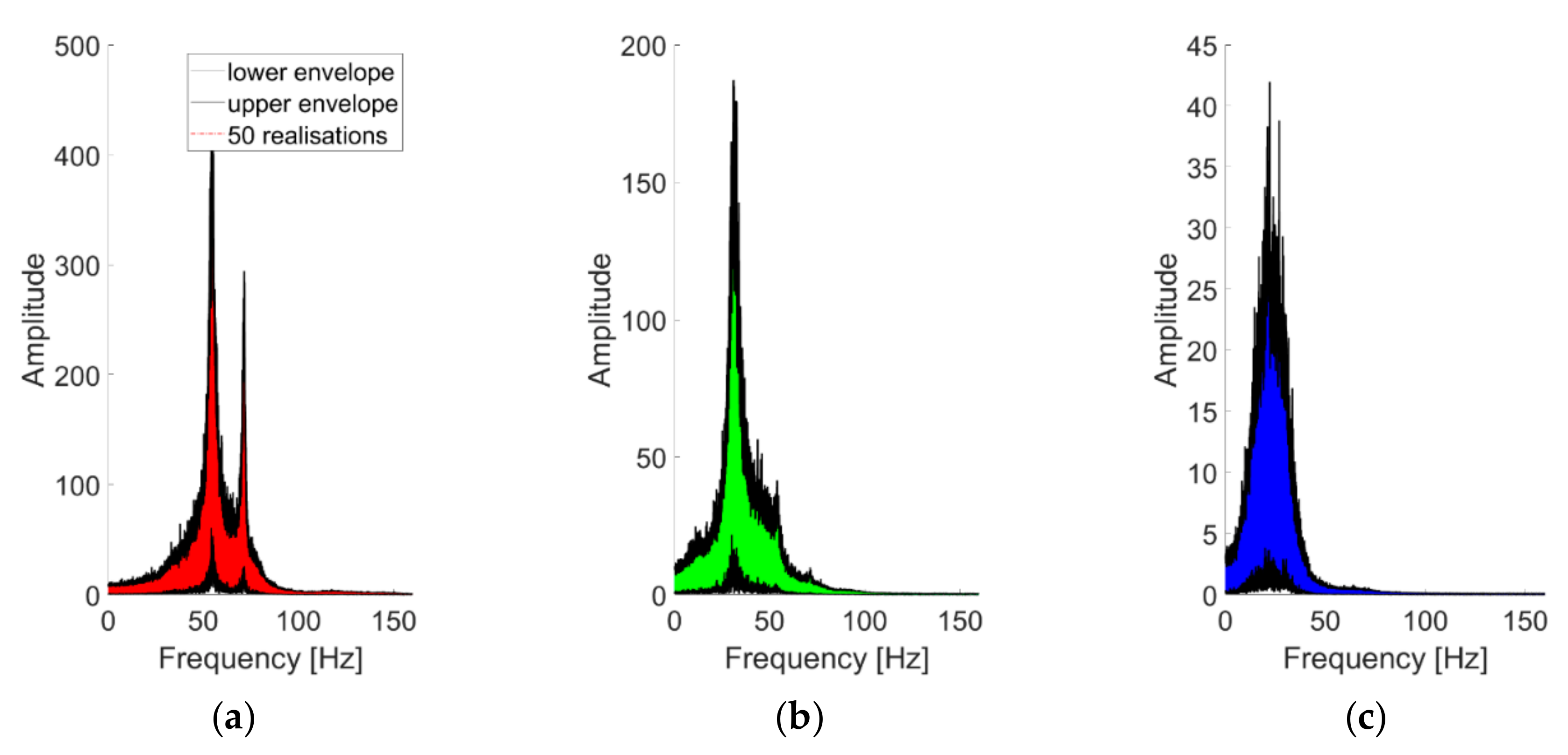
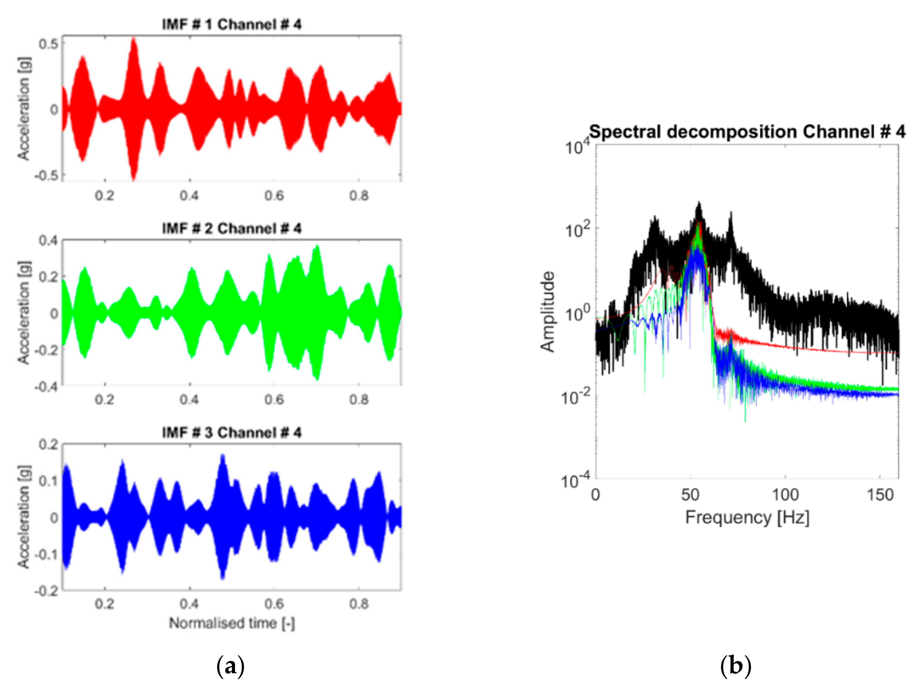
4.3. CEEMDAN IMFs

The CEEMDAN is the only procedure that automatically set the number of its IMFs. The exact number was found to vary depending on the structural conditions. Considering all realisations, channels, and cases, the range spans from a minimum of 11 IMFs (extracted <1% of the times) to a maximum of 15 (3.41%). The decomposition returned 12 or 13 IMFs with an overall occurrence respectively of 41.12% and 48.74%. Results with >15 IMFs (2.35% of the total) can be safely considered as outliers; these happened very often in cases #14 (and to a lesser extent in #13, #15, #16, and #17), due to the noise-like nonlinear distortions being modelled as signal components, reaching 50 IMFs or more. This demonstrates that even with all the improvements with respect to the standard EMD, the CEEMDAN algorithm still suffers an over-decomposition issue. These non-physical IMFs severely hampers the capabilities of the CEEMDAN algorithm.

In all cases, only a few of the first IMFs are of practical interest, as can be seen from Figure 10, which reports the resulting modes in the time and frequency domains for the linear baseline. The first IMF englobes the 2nd and the 3rd eigenmodes of the structure, while the second IMF mostly captures the 1st mode. Thus, the algorithm failed to separate the LNMs of the system.

Any IMF after the third one has a much lower amplitude, and its energy content is bounded to the lower frequencies. These components can even be removed for denoising purposes. Therefore, only $K=1,2,$ and 3 will be discussed in more detail hereinafter.

Regarding the instantaneous frequency, the IFs of the first two IMFs were found to be almost stable as expected, while the other extracted modes are subject to fluctuations that do not have physical meaning.

Regarding the effects of filtering, removing the frequencies out of the input range ($f<20$ Hz and $>150$ Hz) was not particularly beneficial nor detrimental for the CEEMDAN algorithm. The number of the extracted IMFs was not sensibly reduced. The first modes were limitedly affected, while residual IMFs changed noticeably in both the frequency and the time domain; however, these latter components are of almost null utility for SHM purposes whatsoever.

To investigate the statistical stability of the procedure, the first three IMFs as extracted from 50 realisations of the baseline scenario are superimposed in Figure 11. The three components show a good consistency for the several repetitions; the same considerations can be extended to all the linear (damaged or undamaged cases). The nonlinear case showed a much higher variability, especially for IMF #1.

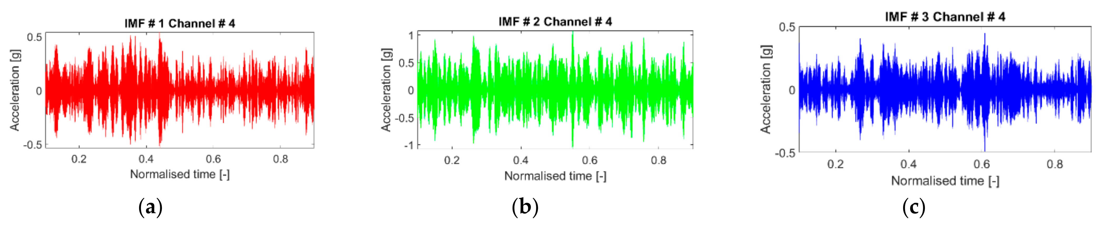
4.4. HVD IMFs

For $K=3$, Figure 12b represents the spectral decomposition of the response at the channels considered for case #1 (linear baseline). These modes are portrayed one by one in the time domain in Figure 12a (notice the different scales on the y-axis). The HVD-extracted IMFs are not similar to the structure’s eigenmodes, as foreseeable, since this decomposition is energy-related rather than frequency-related. All the extracted IMFs have basically the same frequency support, surrounding the main frequency peak (i.e., the 2nd natural frequency of the system). This is most probably because even after the subtraction of the main component, the frequency corresponding to this vibrational mode remains the most prominent energy-wise. This point reverberates in the effects of varying K, as represented in Figure 13. The first IMF to be extracted coincides with the 2nd natural frequency of the structure. Further increasing the value of K does not add useful information about the other two vibrational modes. The reason is the one highlighted above and represented in Figure 13d. After seven iterations, the energy distribution of the residual signal is still qualitatively similar to the original one frequency-wise; hence, any new IMF is extracted around the same ${\omega }_k$ at $\approx$54 Hz.

The impact of the nonlinear distortions in HVD-extracted IMFs is less evident at first sight than for CEEMDAN-extracted IMFs. Generally, the IMFs’ energy distribution in the frequency domain is comparable with the ones of the linear cases. This can be explained since a major part of the IMFs’ energy is bandlimited in a portion of the spectrum less directly affected by the nonlinearity (this point will be further addressed in the next subsections). Therefore, this finding is specific to the dataset considered here and cannot be generalised.

The IF time histories are quite unstable, with fluctuations of more than $\pm 10$ Hz. Moreover, due to the known limitations of the HT, the identifications near the signal ends are unreliable.

For what concerns the filtering, at least for the case study here investigated, this did not generate any noticeable improvement or counterproductive effect, with the resulting IMFs having inconsequential differences in the frequency domain (even if slightly more pronounced and potentially non-negligible in the time domain).

To conclude, the intra-scenario variability is addressed in Figure 14. The IMFs are consistent for the 50 slightly different inputs when applied to the same structural configuration, with the variability slightly larger at the lower frequencies. The same findings apply to the damaged and nonlinear cases as well.

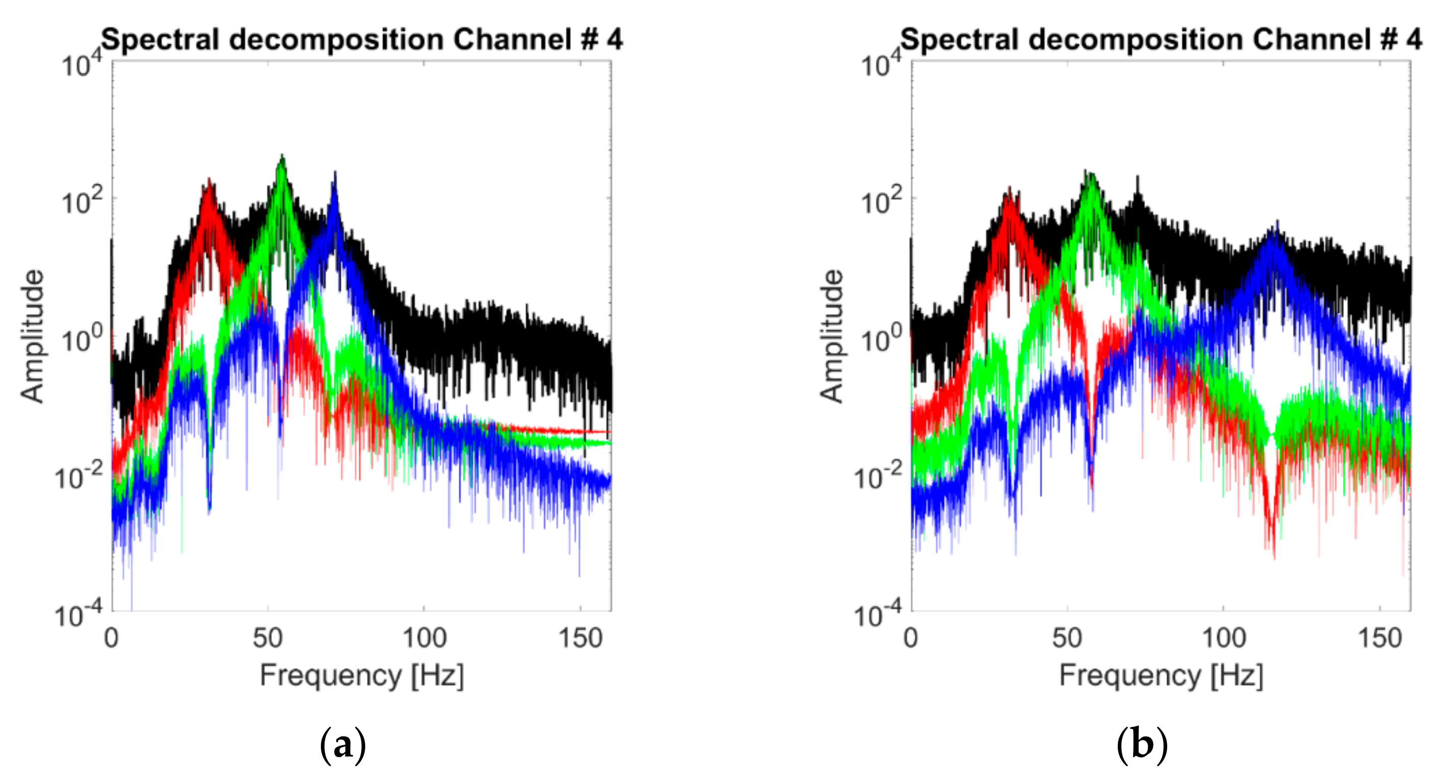
4.5. VMD IMFs

The discussion about the VMD band-limited IMFs follows the same steps seen in the subsections before. The IMFs extracted at the fourth channel for the baseline scenario are individually portrayed in Figure 15. Figure 16a shows the spectral decomposition of the corresponding PSD. In comparison with the HVD and CEEMDAN, the extracted IMFs are very similar to the LNMs of the structure. However, there are some exceptions: for instance, in the nonlinear case #14, for channel output #4, the algorithm fails to properly isolate the third vibrational mode (Figure 16b), capturing instead a superharmonic peak at circa 115 Hz. The third eigenmode was eventually isolated by increasing $K$ to 4.

The investigation on varying the parameter K is shown in Figure 17. The VMD algorithm reacts well in the sense that it captures a good approximation of the first eigenmode for $K=1$ and a good estimation of the other two eigenmodes for $K=2$ and $K=3$. On the other hand, increasing $K\ge 3$ produces no physically meaningful modes in the linear case of Figure 17c, while it was found to successfully isolate super- and sub-harmonics in other nonlinear scenarios, as explained before.

The IF time histories of the IMFs were found to be generally very stable and not noticeably affected by the presence of large nonlinear distortions—even the superharmonics, when isolated by increasing $K\ge 4$ in cases #10 to #17, are properly tracked instant by instant. The corresponding centre frequencies also showed good stability for the several recordings.

Unexpectedly, it was observed that filtering out the frequencies below 20 Hz caused the algorithm to not correctly isolate the first natural frequency on some (not frequent) occasions, as reported in Figure 18 for the 3rd channel (baseline case). In this specific case, the issue was solved by reducing the high-pass cut-off frequency to 12 Hz or less. This point suggests that frequency peaks too close to the cut-off frequencies may be more difficult to isolate, which is most probably due to the presence of attenuated content in the nearby frequencies. The same occurrence, while not frequently encountered, was noticed for some nonlinear and damaged scenarios as well. Therefore, the VMD returned overall better results when applied to the signal without filtering it.

Concluding this first discussion about the extracted IMFs, the statistical stability of the VMD results is portrayed in Figure 19 by superposing the 50 realisations for each IMF in the frequency domain. In the linear cases, the identification procedure returns stable and consistent modes, with limited variability amplitude-wise and very limited variability frequency-wise. For the nonlinear scenarios, the mislabeling between the 3rd natural mode and the 1st superharmonic caused a superposition of two distinguished IMFs (Figure 19f). The issue was easily solved by increasing $K$ to 4. This almost completely solved any ambiguity (Figure 19g).

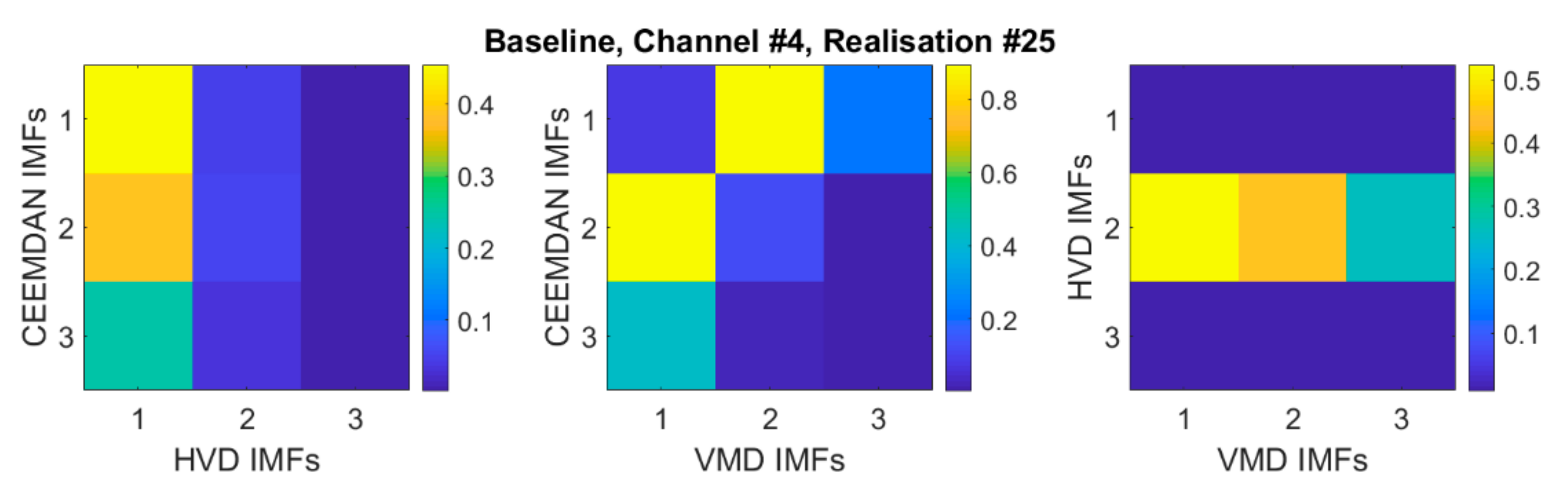
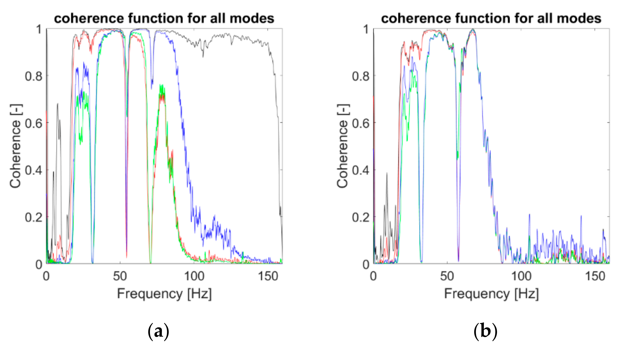
4.6. Comparability of the Extracted Modes

In Figure 20, the IMFs extracted by means of the CEEMDAN, HVD, and VMD algorithms are compared to establish if and how much similar they are. This was done by considering the correlation coefficient of each signal pair. The reported results refer to the 25th realisation of the undamaged baseline. From the first matrix, it is visible that for the CEEMDAN and HVD methods, the first IMF is the most similar, even if it is still quite different in absolute terms. The second matrix shows instead how the 1st CEEEMDAN IMF compares very well with the 2nd VMD IMF and vice versa. This is coherent with what has been observed before, as the 1st CEEMDAN IMF englobed both the 2nd and the 3rd eigenmodes, while the 2nd CEEMDAN IMF corresponded roughly to the 1st normal mode. Finally, from the last matrix (on the right), one can notice the second LNM, which is recurrent in all HVD modes and captured by the 2nd IMF of the VMD approach. Similar outcomes were encountered for the other scenarios as well.

4.7. Sensitivity of the Extracted IMFs to Damage

Having established the similarities and differences among the IMFs extracted with the three different techniques, it is now necessary to address their reliability as DSFs for Machine Learning. All the proposed techniques allow for precise time-frequency analysis, which is useful for both real-time continuous monitoring and the a posteriori analyses of short-timed extreme conditions such as earthquakes, explosions, typhoons etc. on the structure.

Damage can be detected in several modes. The frequency-based approaches rely on changes in the PSD distribution. Figure 21 highlights how this is easily doable with CEEMDAN, HVD, and VMD-extracted IMFs. Figure 21a shows the CEEMDAN IMFs, where the major frequency shifts (linked to the 2nd and 3rd natural frequencies) are absorbed into the first IMF for all the damaged scenarios. In Figure 21b, all the HVD BLIMFs are very sensitive to the changes of case #5 and insensitive to the ones of case #7, as they are all centred around the 2nd eigenfrequency. This proves that different IMFs extracted with different techniques react more or less markedly to specific typologies and locations of the damage. For instance, for case #5 (linear response, strongly damaged at the 1st inter-storey), the frequency shift of the 2nd VMD BLIMF is clear (Figure 21c), while this is less evident for the 3rd and the 1st BLIMFs. In case #7 (Figure 21d), the damage-induced effects are prominent for the 3rd BLIMF and almost unnoticeable in the other two. This also reflects the different positions of the stiffness reduction. For these reasons, the extracted IMFs can be even used for more specific damage assessment tasks, such as damage localisation, exploiting their differences and peculiarities as generally done for modal parameters and especially mode shapes [48]. In this sense, mode shape-based approaches rely on the vibrational modes of the structure, which can be in turn obtained from the modal components of the signal. Considering the VMD-extracted BLIMFs as a sufficiently good approximation of the investigated system’s eigencomponents, the structural deflection shapes can be qualitatively estimated from them. Figure 22 shows an example of damage localisation, exploiting the deflection shapes corresponding to the first identified VMD BLIMF and the known location of the four output channels. However, proper damage localisation using these extracted features will need further investigation before being established beyond any reasonable doubts.

Finally, assuming the damage as a pointwise source of nonlinearity in an otherwise linear system, any nonlinear test can be run over the single IMFs as normally done for the whole signal. The magnitude-squared coherence function [62], defined between the input force and the output channel #4, is reported in Figure 23 for the three VMD-extracted BLIMFs compared to the whole signal. It is evident how, for case #14 (i.e. the one with the strongest nonlinearity), the 3rd BLIMF is much more affected than the 2nd IMF, while the first component is almost unaltered. This reflects what was seen previously, since a large portion of the frequency support of the 3rd BLIMF falls in the distorted region (roughly from 70 Hz upward). This aspect will be further recalled in the following subsection as well.

Therefore, depending on the intended use, several IMFs, especially the ones obtained through VMD, can be exploited to discern (or even locate) operational changes, the presence of nonlinearities, or stiffness reductions.

4.8. Uses for ML-Based SHM

This last part aims to illustrate how the DSFs extracted from the signal components can be used to train an ML algorithm to perform automatically continuous monitoring. Indeed, algorithms such as the EMD are appreciated for pattern recognition problems [63], which are the basis for ML-based SHM.

To replicate the settings of Ref. [59], the recorded accelerations from Cases #1, #3, #7, #14, and #17 have been concatenated. This is intended to simulate time-varying structural changes such as operational conditions (with mass overloads) and damage inception (both linear and nonlinear). The resulting modes are portrayed in Figure 24. As before, only the response at the fourth (top storey) channel for the 25th WGN input is reported for brevity. It can be noticed that the amplitude of the HVD IMFs is much lower than the one of their VMD and CEEMDAN counterparts.

The IF time histories of the IMFs extracted from the undamaged baseline have been used to define a “normality” condition for the target structure. To ensure the replicability of the results, a simple yet effective approach, the Gaussian Process Regression (GPR; [64]), has been utilised. This approach is well-known in the SHM community for surrogate modelling and has been proved valid by decades of extensive use [65,66,67]. All 50 realisations have been used to define the normality model and the corresponding $3 \sigma$ thresholds. Only for the HVD method, to avoid the HT edge effects, 5% of the data at both ends have been removed from the training dataset (this step was unnecessary for both CEEMDAN and VMD).

Figure 25 shows the results of this analysis. As explained before, the intent of this paper is not to address any specific ML technique for anomaly detection; the aim is to compare the results obtained from the use of mode-related features. In this simple case presented here, the CEEMDAN-extracted IMFs (Figure 25a) are the only ones with noticeable (even if very small) fluctuations of the IF in their baseline model. The first IMF seems to be relatively sensitive to damage and structural changes, as it slightly deviates from the predicted value (dash-dotted grey line) for case #7 and more markedly for the nonlinear case #14. However, it falls mostly at any instant in the 99.7% confidence interval (grey area). The 2nd and 3rd IMFs seem to be unchanged by the added mass or the inserted pointwise source of nonlinearity. This can be both an advantage (e.g., for masonry structures, where many material and geometrical nonlinearities cause noise-like, damage-unrelated distortions) or a limitation (e.g., being insensitive to breathing cracks’ effects). For the 2nd IMF, it is noticeable, as decreasing the stiffness causes the DSF to trespass the threshold value for a few instants in case #7. Nevertheless, such deviation from the normality model is arguably too small and time limited to signify damage with good confidence.

The HVD-extracted modes (Figure 25b) did not show good potential for damage detection, remaining unaltered for varying structural conditions and quite unstable overall. VMD-extracted modes (Figure 25c) showed more encouraging results. The IF of the first IMF differs appreciably from the expected value for case #7 (linear damage), even if it is still in the $3\sigma$ range almost everywhere. On the other hand, it is quite unaffected by the presence of the nonlinear distortions and by the added masses. Conversely, mode #2 is more affected by the added mass (case #3) than by the reduced stiffness (case #7), even if the deviation from the predicted values is well under the alarm threshold. On the other hand, it is quite sensitive to the most nonlinear scenario of case #14. Finally, the third IMF is the most sensitive one to both linear and nonlinear damage, trespassing the confidence interval for case #7 and even more markedly for case #14, while remaining under the threshold for the cases with the additional masses. This finding confirms what was reported in Ref. [59], where the bumper’s impacts were found to affect the most the third eigenmode of the structure.

5. Discussion and Conclusions

In this work, data-adaptive mode decomposition techniques have been investigated for SHM purposes. Departing from the broad set of proposals available in the scientific literature, the selection was narrowed down to the three methods—the EMD, HVD, and VMD algorithms. These candidates have been considered to be representative of the whole current state of the art, due to their popularity and the several similarities shared with other strictly related approaches.

The three algorithms have been methodically investigated and compared. Their theoretical and practical strong and weak points have been thoroughly discussed. All the parameters and settings have been reported for the reproducibility of the results.

The examined IF time histories were found to be suitable for ML-based damage detection, even in the presence of noise-like distortions induced by structural nonlinearities and when concatenated to mimic sudden structural changes and signal nonstationarity. The key findings of this comparative study can be enlisted as follows:

• Regarding the choice between the data-driven or manual selection of the number $K$ of modes to be extracted, for structural engineering purposes, the second option should be preferred. The number of relevant vibrational modes of a target structure can be easily estimated or guessed; on the other hand, having a fixed number of modes greatly simplifies the comparison between different measurements. This also makes the detection of (most likely damage-related) anomalies easier and more reliable.
• When comparing the IMFs extracted from different recordings, it is necessary to check their comparability to avoid blunders.
• Filtering the acceleration THs of the structure under random excitations did not improve significantly any of the tested algorithms, or at least not for the specific case investigated here.
• The CEEMDAN algorithm can be used to isolate the most important characteristics of the target signal, yet it is greatly affected by measurement noise and nonlinear distortions.
• The HVD is better suited for time-domain applications rather than frequency-domain ones. It has a remarkable role for nonlinear SDoF systems where it can efficiently isolate distinct (linear or nonlinear) terms for forced or free vibrations. It is also well suited for the analysis of nonstationary responses to external impulses and the extraction of energy-related damage sensitive features. However, it is less apt for systems with multiple degrees of freedom and/or to track damage-related frequency shifts.
• The VMD approach performed overall better than the CEEMDAN and HVD techniques for tracking frequency shifts.

To conclude, all the reviewed approaches have their strong points that can serve specific tasks. For vibration-based SHM purposes, the authors of this comparative analysis will finally suggest VMD as a viable option with several noteworthy advantages and few practical and theoretical limitations. Hopefully, this comparative analysis on a well-documented experimental case study will provide some suggestions for the practitioners in search of the most fitting approach for their applications, as well as some hints for researchers committed to developing new alternatives.

The authors are committed to performing similar comparative analyses for other promising (even if slightly less known) algorithms and also for wavelet-based approaches. Real-time applications will be of great interest as well.

References

- Farrar, C.R.; Worden, K. Structural Health Monitoring: A Machine Learning Perspective; John Wiley & Sons: Toronto, ON, Canada, 2013. [Google Scholar]
- Salawu, O. Detection of structural damage through changes in frequency: A review. Eng. Struct. 1997, 19, 718–723. [Google Scholar] [CrossRef]
- Bhowmik, B.; Tripura, T.; Hazra, B.; Pakrashi, V. First-Order Eigen-Perturbation Techniques for Real-Time Damage Detection of Vibrating Systems: Theory and Applications. Appl. Mech. Rev. 2019, 71. [Google Scholar] [CrossRef]
- Bhowmik, B.; Krishnan, M.; Hazra, B.; Pakrashi, V. Real-time unified single- and multi-channel structural damage detection using recursive singular spectrum analysis. Struct. Health Monit. 2018, 18, 563–589. [Google Scholar] [CrossRef]
- Iakovidis, I.; Cross, E.J.; Worden, K. A principled multiresolution approach for signal decomposition. J. Phys. Conf. Ser. 2018, 1106, 012001. [Google Scholar] [CrossRef] [Green Version]
- Feng, Z.; Zhang, N.; Zuo, M.J. Adaptive Mode Decomposition Methods and Their Applications in Signal Analysis for Machinery Fault Diagnosis: A Review with Examples. IEEE Access 2017, 5, 24301–24331. [Google Scholar] [CrossRef]
- Huang, N.E.; Shen, Z.; Long, S.R.; Wu, M.C.; Shih, H.H.; Zheng, Q.; Yen, N.C.; Tung, C.C.; Liu, H.H. The empirical mode decomposition and the Hilbert spectrum for nonlinear and non-stationary time series analysis. Proc. R. Soc. A Math. Phys. Eng. Sci. 1998, 454, 903–995. [Google Scholar] [CrossRef]
- Smith, J.S. The local mean decomposition and its application to EEG perception data. J. R. Soc. Interface 2005, 2, 443–454. [Google Scholar] [CrossRef] [PubMed]
- Zheng, J.; Cheng, J.; Yang, Y. A rolling bearing fault diagnosis approach based on LCD and fuzzy entropy. Mech. Mach. Theory 2013, 70, 441–453. [Google Scholar] [CrossRef]
- Feldman, M. Time-varying vibration decomposition and analysis based on the Hilbert transform. J. Sound Vib. 2006, 295, 518–530. [Google Scholar] [CrossRef]
- Gilles, J. Empirical Wavelet Transform. IEEE Trans. Signal Process. 2013, 61, 3999–4010. [Google Scholar] [CrossRef]
- Dragomiretskiy, K.; Zosso, D. Variational Mode Decomposition. IEEE Trans. Signal Process. 2014, 62, 531–544. [Google Scholar] [CrossRef]
- Frei, M.G.; Osorio, I. Intrinsic time-scale decomposition: Time–frequency–energy analysis and real-time filtering of non-stationary signals. Proc. R. Soc. A Math. Phys. Eng. Sci. 2006, 463, 321–342. [Google Scholar] [CrossRef]
- Barbosh, M.; Singh, P.; Sadhu, A. Empirical mode decomposition and its variants: A review with applications in structural health monitoring. Smart Mater. Struct. 2020, 29, 3001. [Google Scholar] [CrossRef]
- Isham, M.F.; Leong, M.S.; Lim, M.H.; Zakaria, M.K. A Review on Variational Mode Decomposition for Rotating Machinery Diagnosis; EDP Sciences: Les Ulis, France, 2019; Volume 255. [Google Scholar] [CrossRef]
- Figueiredo, E.; Park, G.; Farrar, C.R.; Worden, K.; Figueiras, J. Machine learning algorithms for damage detection under operational and environmental variability. Struct. Health Monit. 2010, 10, 559–572. [Google Scholar] [CrossRef]
- Rilling, G.; Flandrin, P.; Goncalves, P.; Lilly, J.M. Bivariate Empirical Mode Decomposition. IEEE Signal Process. Lett. 2007, 14, 936–939. [Google Scholar] [CrossRef] [Green Version]
- Rehman, N.; Mandic, D.P. Multivariate empirical mode decomposition. Proc. R. Soc. A Math. Phys. Eng. Sci. 2009, 466, 1291–1302. [Google Scholar] [CrossRef]
- McNeill, S. Decomposing a signal into short-time narrow-banded modes. J. Sound Vib. 2016, 373, 325–339. [Google Scholar] [CrossRef]
- Yang, J.N.; Lei, Y.; Pan, S.; Huang, N. System identification of linear structures based on Hilbert-Huang spectral analysis. Part 1: Normal modes. Earthq. Eng. Struct. Dyn. 2003, 32, 1443–1467. [Google Scholar] [CrossRef]
- Shi, Z.Y.; Law, S.S. Identification of Linear Time-Varying Dynamical Systems Using Hilbert Transform and Empirical Mode Decomposition Method. J. Appl. Mech. 2006, 74, 223–230. [Google Scholar] [CrossRef]
- Yu, D.J.; Ren, W.X. EMD-based stochastic subspace identification of structures from operational vibration measurements. Eng. Struct. 2005, 27, 1741–1751. [Google Scholar] [CrossRef]
- Chen, J.; Xu, Y.; Zhang, R. Modal parameter identification of Tsing Ma suspension bridge under Typhoon Victor: EMD-HT method. J. Wind. Eng. Ind. Aerodyn. 2004, 92, 805–827. [Google Scholar] [CrossRef]
- Chen, J. Application of Empirical Mode Decomposition in Structural Health Monitoring: Some Experience. Adv. Adapt. Data Anal. 2009, 1, 601–621. [Google Scholar] [CrossRef]
- Lei, Y.; Lin, J.; He, Z.; Zuo, M.J. A review on empirical mode decomposition in fault diagnosis of rotating machinery. Mech. Syst. Signal Process. 2013, 35, 108–126. [Google Scholar] [CrossRef]
- Liu, J.; Wang, X.; Yuan, S.; Li, G. On Hilbert-Huang Transform Approach for Structural Health Monitoring. J. Intell. Mater. Syst. Struct. 2006, 17, 721–728. [Google Scholar] [CrossRef]
- Huang, E.N.; Shen, S.S.P. Hilbert-Huang Transform and Its Applications; World Scientific Pub Co Pte Lt: Chennai, India, 2005; Volume 16. [Google Scholar]
- Kizhner, S.; Flatley, T.; Huang, N.E.; Blank, K.; Conwell, E. On the Hilbert-Huang transform data processing system development. In Proceedings of the 2004 IEEE Aerospace Conference Proceedings (IEEE Cat. No.04TH8720), Big Sky, MT, USA, 6–13 March 2004; pp. 1961–1978. [Google Scholar] [CrossRef] [Green Version]
- Wu, Z.; Huang, N.E.; Shen, S.S.P. Statistical Significance Test of Intrinsic Mode Functions. Hilbert–Huang Transform Appl. 2014, 149–169. [Google Scholar] [CrossRef] [Green Version]
- Colominas, M.A.; Schlotthauer, G.; Torres, M.E. Improved complete ensemble EMD: A suitable tool for biomedical signal processing. Biomed. Signal Process. Control 2014, 14, 19–29. [Google Scholar] [CrossRef]
- Wu, Z.; Huang, N.E. Ensemble Empirical Mode Decomposition: A Noise-Assisted Data Analysis Method. Adv. Adapt. Data Anal. 2009, 1, 1–41. [Google Scholar] [CrossRef]
- Torres, M.E.; Colominas, M.A.; Schlotthauer, G.; Flandrin, P. A complete ensemble empirical mode decomposition with adaptive noise. In Proceedings of the 2011 IEEE International Conference on Acoustics, Speech and Signal Processing (ICASSP), Prague, Czech Republic, 22–27 May 2011; pp. 4144–4147. [Google Scholar] [CrossRef]
- Feldman, M. Hilbert transform in vibration analysis. Mech. Syst. Signal Process. 2011, 25, 735–802. [Google Scholar] [CrossRef]
- Huang, N.E.; Wu, Z.; Long, S.R.; Arnold, K.C.; Chen, X.; Blank, K. On Instantaneous Frequency. Adv. Adapt. Data Anal. 2009, 1, 177–229. [Google Scholar] [CrossRef]
- Londoño, J.M.; Neild, S.A.; Cooper, J.E. Identification of backbone curves of nonlinear systems from resonance decay responses. J. Sound Vib. 2015, 348, 224–238. [Google Scholar] [CrossRef] [Green Version]
- Neild, S.; McFadden, P.; Williams, M. A review of time-frequency methods for structural vibration analysis. Eng. Struct. 2003, 25, 713–728. [Google Scholar] [CrossRef]
- Civera, M.; Fragonara, L.Z.; Surace, C. Using Video Processing for the Full-Field Identification of Backbone Curves in Case of Large Vibrations. Sensors 2019, 19, 2345. [Google Scholar] [CrossRef] [PubMed] [Green Version]
- Maragos, P.; Kaiser, J.; Quatieri, T. On amplitude and frequency demodulation using energy operators. IEEE Trans. Signal Process. 1993, 41, 1532–1550. [Google Scholar] [CrossRef]
- Junsheng, C.; Dejie, Y.; Yü, Y. The application of energy operator demodulation approach based on EMD in machinery fault diagnosis. Mech. Syst. Signal Process. 2007, 21, 668–677. [Google Scholar] [CrossRef]
- Zheng, J.; Pan, H.; Yang, S.; Cheng, J. Adaptive parameterless empirical wavelet transform based time-frequency analysis method and its application to rotor rubbing fault diagnosis. Signal Process. 2017, 130, 305–314. [Google Scholar] [CrossRef]
- Feldman, M. Hilbert Transform Applications in Mechanical Vibration; John Wiley & Sons: Toronto, ON, Canada, 2011. [Google Scholar]
- Feldman, M. Hilbert Transform, Envelope, Instantaneous Phase, and Frequency. Encycl. Struct. Health Monit. 2008. [Google Scholar] [CrossRef]
- Feldman, M. Considering high harmonics for identification of non-linear systems by Hilbert transform. Mech. Syst. Signal Process. 2007, 21, 943–958. [Google Scholar] [CrossRef]
- Feldman, M. Identification of weakly nonlinearities in multiple coupled oscillators. J. Sound Vib. 2007, 303, 357–370. [Google Scholar] [CrossRef]
- Noël, J.; Kerschen, G. Nonlinear system identification in structural dynamics: 10 more years of progress. Mech. Syst. Signal Process. 2017, 83, 2–35. [Google Scholar] [CrossRef]
- Boashash, B. Estimating and interpreting the instantaneous frequency of a signal. I. Fundamentals. Proc. IEEE 1992, 80, 520–538. [Google Scholar] [CrossRef]
- Braun, S.; Feldman, M. Decomposition of non-stationary signals into varying time scales: Some aspects of the EMD and HVD methods. Mech. Syst. Signal Process. 2011, 25, 2608–2630. [Google Scholar] [CrossRef]
- Civera, M.; Fragonara, L.Z.; Surace, C. An experimental study of the feasibility of phase-based video magnification for damage detection and localisation in operational deflection shapes. Strain 2020, 56, 2336. [Google Scholar] [CrossRef]
- Ni, P.; Li, J.; Hao, H.; Xia, Y.; Wang, X.; Lee, J.M.; Jung, K.H. Time-varying system identification using variational mode decomposition. Struct. Control Health Monit. 2018, 25, 2175. [Google Scholar] [CrossRef]
- Bagheri, A.; Ozbulut, O.E.; Harris, D.K. Structural system identification based on variational mode decomposition. J. Sound Vib. 2018, 417, 182–197. [Google Scholar] [CrossRef]
- Wang, Y.; Markert, R.; Xiang, J.; Zheng, W. Research on variational mode decomposition and its application in detecting rub-impact fault of the rotor system. Mech. Syst. Signal Process. 2015, 60, 243–251. [Google Scholar] [CrossRef]
- Carson, J. Notes on the Theory of Modulation. Proc. IRE 1922, 10, 57–64. [Google Scholar] [CrossRef] [Green Version]
- Liu, W.; Cao, S.; Chen, Y. Applications of variational mode decomposition in seismic time-frequency analysis. Geophysics 2016, 81, V365–V378. [Google Scholar] [CrossRef]
- Huang, Y.; Yan, C.J.; Xu, Q. On the difference between empirical mode decomposition and Hilbert vibration decomposition for earthquake motion records. In Proceedings of the 15th World Conference on Earthquake Engineering, Lisbon, Portugal, 24–28 September 2012. [Google Scholar]
- Aneesh, C.; Kumar, S.; Hisham, P.; Soman, K. Performance Comparison of Variational Mode Decomposition over Empirical Wavelet Transform for the Classification of Power Quality Disturbances Using Support Vector Machine. Procedia Comput. Sci. 2015, 46, 372–380. [Google Scholar] [CrossRef] [Green Version]
- Pontillo, A.; Hayes, D.; Dussart, G.X.; Matos, G.E.L.; Carrizales, M.A.; Yusuf, S.Y.; Lone, M.M. Flexible High Aspect Ratio Wing: Low Cost Experimental Model and Computational Framework. In Proceedings of the 2018 AIAA Atmospheric Flight Mechanics Conference, American Institute of Aeronautics and Astronautics, Atlanta, GA, USA, 25–29 June 2018. [Google Scholar]
- Civera, M.; Fragonara, L.Z.; Surace, C. A Computer Vision-Based Approach for Non-Contact Modal Analysis and Finite Element Model Updating; Springer International Publishing: New York, NY, USA, 2021; pp. 481–493. [Google Scholar]
- Civera, M.; Ferraris, M.; Ceravolo, R.; Surace, C.; Betti, R. The Teager-Kaiser Energy Cepstral Coefficients as an Effective Structural Health Monitoring Tool. Appl. Sci. 2019, 9, 5064. [Google Scholar] [CrossRef] [Green Version]
- Figueiredo, E.; Park, G.; Figueiras, J.; Farrar, C.; Worden, K. Structural Health Monitoring Algorithm Comparisons Using Standard Data Sets; Office of Scientific and Technical Information (OSTI): Oak Ridge, TN, USA, 2009.
- Pugno, N.; Surace, C.; Ruotolo, R. Evaluation of the Non-Linear Dynamic Response to Harmonic Excitation of a Beam with Several Breathing Cracks. J. Sound Vib. 2000, 235, 749–762. [Google Scholar] [CrossRef] [Green Version]
- Panda, S.; Tripura, T.; Hazra, B. First-Order Error-Adapted Eigen Perturbation for Real-Time Modal Identification of Vibrating Structures. J. Vib. Acoust. 2021, 143, 1–25. [Google Scholar] [CrossRef]
- Kay, S.M. Modern Spectral Estimation: Theory and Application; Pearson Education: London, UK, 1988. [Google Scholar]
- Klionskiy, D.M.; Kaplun, D.I.; Geppener, V.V. Empirical Mode Decomposition for Signal Preprocessing and Classification of Intrinsic Mode Functions. Pattern Recognit. Image Anal. 2018, 28, 122–132. [Google Scholar] [CrossRef]
- Rasmussen, C.E. Gaussian Processes in Machine Learning. In Summer School on Machine Learning; Springer: Cham, Switzerland, 2004; pp. 63–71. [Google Scholar] [CrossRef] [Green Version]
- Civera, M.; Surace, C.; Worden, K. Detection of Cracks in Beams Using Treed Gaussian Processes. In Proceedings of the Conference of Society for Experimental Mechanics Series; Springer International Publishing, Garden Grove, CA, USA, 30 January–2 February 2017; Volume 19, pp. 85–97. [Google Scholar]
- Martucci, D.; Civera, M.; Surace, C.; Worden, K. Novelty Detection in a Cantilever Beam using Extreme Function Theory. J. Phys. Conf. Ser. 2018, 1106, 2027. [Google Scholar] [CrossRef] [Green Version]
- Civera, M.; Boscato, G.; Fragonara, L.Z. Treed gaussian process for manufacturing imperfection identification of pultruded GFRP thin-walled profile. Compos. Struct. 2020, 254, 2882. [Google Scholar] [CrossRef]
- Rato, R.; Ortigueira, M.; Batista, A. On the HHT, its problems, and some solutions. Mech. Syst. Signal Process. 2008, 22, 1374–1394. [Google Scholar] [CrossRef] [Green Version]
- Klionskiy, D.; Kupriyanov, M.; Kaplun, D. Mikhail Signal denoising based on empirical mode decomposition. J. Vibroeng. 2017, 19, 5560–5570. [Google Scholar] [CrossRef]
- Ricci, R.; Pennacchi, P. Diagnostics of gear faults based on EMD and automatic selection of intrinsic mode functions. Mech. Syst. Signal Process. 2011, 25, 821–838. [Google Scholar] [CrossRef] [Green Version]
- Huang, N.E.; Shen, Z.; Long, S.R. A New View of Nonlinear Water Waves: The Hilbert Spectrum. Annu. Rev. Fluid Mech. 1999, 31, 417–457. [Google Scholar] [CrossRef] [Green Version]
- Rilling, G.; Flandrin, P.; Gonçalves, P. On Empirical Mode Decomposition and Its Algorithms. 2003. Available online: https://hal.inria.fr/inria-00570628 (accessed on 14 September 2020).
- Junsheng, C.; Dejie, Y.; Yu, Y. Research on the intrinsic mode function (IMF) criterion in EMD method. Mech. Syst. Signal Process. 2006, 20, 817–824. [Google Scholar] [CrossRef]
- Flandrin, P.; Rilling, G.; Goncalves, P. Empirical Mode Decomposition as a Filter Bank. IEEE Signal Process. Lett. 2004, 11, 112–114. [Google Scholar] [CrossRef] [Green Version]
- Dätig, M.; Schlurmann, T. Performance and limitations of the Hilbert–Huang transformation (HHT) with an application to irregular water waves. Ocean Eng. 2004, 31, 1783–1834. [Google Scholar] [CrossRef]
- Rilling, G.; Flandrin, P. One or Two Frequencies? The Empirical Mode Decomposition Answers. IEEE Trans. Signal Process. 2008, 56, 85–95. [Google Scholar] [CrossRef] [Green Version]
- Wang, Y.H.; Yeh, C.H.; Young, H.W.V.; Hu, K.; Lo, M.T. On the computational complexity of the empirical mode decomposition algorithm. Phys. A Stat. Mech. Appl. 2014, 400, 159–167. [Google Scholar] [CrossRef]
- Voznesenskiy, A.; Kaplun, D. Adaptive Signal Processing Algorithms Based on EMD and ITD. IEEE Access 2019, 7, 171313–171321. [Google Scholar] [CrossRef]
- Fontugne, R.; Borgnat, P.; Flandrin, P. Online Empirical Mode Decomposition. In Proceedings of the 2017 IEEE International Conference on Acoustics, Speech and Signal Processing (ICASSP), New Orleans, LA, USA, 5–9 March 2017; pp. 4306–4310. [Google Scholar]
- Qiang, Z.G.; Wei, M.Z.; Quan, X.G.; Jie, W.D. On the difference between empirical mode decomposition and wavelet decomposition in the nonlinear time series. Acta Phys. Sin. 2005, 54, 3947–3957. [Google Scholar] [CrossRef]
- Chen, S.; Dong, X.; Peng, Z.; Zhang, W.; Meng, G. Nonlinear Chirp Mode Decomposition: A Variational Method. IEEE Trans. Signal Process. 2017, 65, 6024–6037. [Google Scholar] [CrossRef]
- Peng, Z.; Tse, P.W.; Chu, F. A comparison study of improved Hilbert–Huang transform and wavelet transform: Application to fault diagnosis for rolling bearing. Mech. Syst. Signal Process. 2005, 19, 974–988. [Google Scholar] [CrossRef]
- Yang, W.; Peng, Z.; Wei, K.; Shi, P.; Tian, W. Superiorities of variational mode decomposition over empirical mode decomposition particularly in time–frequency feature extraction and wind turbine condition monitoring. IET Renew. Power Gener. 2017, 11, 443–452. [Google Scholar] [CrossRef] [Green Version]
- Sharma, H.; Sharma, K. Baseline wander removal of ECG signals using Hilbert vibration decomposition. Electron. Lett. 2015, 51, 447–449. [Google Scholar] [CrossRef]
- Mutlu, A.Y. Detection of epileptic dysfunctions in EEG signals using Hilbert vibration decomposition. Biomed. Signal Process. Control 2018, 40, 33–40. [Google Scholar] [CrossRef]
- Feldman, M. Theoretical analysis and comparison of the Hilbert transform decomposition methods. Mech. Syst. Signal Process. 2008, 22, 509–519. [Google Scholar] [CrossRef]
- Liu, Y.; Yang, G.; Li, M.; Yin, H. Variational mode decomposition denoising combined the detrended fluctuation analysis. Signal Process. 2016, 125, 349–364. [Google Scholar] [CrossRef]
- Sahani, M.; Dash, P.; Samal, D. A real-time power quality events recognition using variational mode decomposition and online-sequential extreme learning machine. Measurement 2020, 157, 107597. [Google Scholar] [CrossRef]