Abstract
Hyperspectral image (HSI) classification is the subject of intense research in remote sensing. The tremendous success of deep learning in computer vision has recently sparked the interest in applying deep learning in hyperspectral image classification. However, most deep learning methods for hyperspectral image classification are based on convolutional neural networks (CNN). Those methods require heavy GPU memory resources and run time. Recently, another deep learning model, the transformer, has been applied for image recognition, and the study result demonstrates the great potential of the transformer network for computer vision tasks. In this paper, we propose a model for hyperspectral image classification based on the transformer, which is widely used in natural language processing. Besides, we believe we are the first to combine the metric learning and the transformer model in hyperspectral image classification. Moreover, to improve the model classification performance when the available training samples are limited, we use the 1-D convolution and Mish activation function. The experimental results on three widely used hyperspectral image data sets demonstrate the proposed model’s advantages in accuracy, GPU memory cost, and running time.
1. Introduction
Hyperspectral image (HSI) classification is a focus point in remote sensing because of its many uses across fields, such as change area detection [1], land-use classification [2,3], and environmental protection [4]. However, because of redundant spectral band information, large data size, and a limited number of training samples, the pixel-wise classification of the hyperspectral image remains a formidable challenge.
Deep learning (DL) has become extremely popular because of its ability to extract features from raw data. It has been applied in computer vision tasks, such as image classification [5,6,7,8], object detection [9], semantic segmentation [10], and facial recognition [11]. As a classical visual classification task, HSI classification has also been influenced by DL. For example, Chen et al. [12] proposed a stacked autoencoder for feature extraction. Ma et al. [13] introduced an updated deep auto-encoder to extract spectral–spatial features. Zhang et al. [14], adopted a recursive autoencoder (RAE) as a high-level feature extractor to produce feature maps from the target pixel neighborhoods. Chen et al. [15], combined deep belief network (DBN) and restricted Boltzmann machine (RBM) for hyperspectral image classification.
However, these methods extract the features with destroying the initial spatial structure. Because convolutional neural networks (CNNs) can extract spatial features without destroying the original structure, new methods based on CNNs have been introduced. For example, Chen et al. [16] designed a novel 3-D-CNN model with regularization for HSI classification. Roy et al. [17] proposed a hybrid 3-D and 2-D model for HSI classification.
In addition to modifying the CNN structure, deep metric learning (DML) has been applied to improve CNN classification performance. The metric learning loss term was introduced to the CNN objective function to enhance the model’s discriminative power. Cheng et al. [18] designed a DML method based on existing CNN models for remote sensing image classification. Guo et al. [19] proposed a DML framework for HSI spectral–spatial feature extraction and classification.
Recently, another deep learning model, the transformer, has been applied for computer vision tasks. In Reference [20], transformers were proposed for machine translation and became the state-of-art model in many natural language processing (NLP) tasks. In Reference [21], the transformer network’s direct application, Vision Transformer, to image recognition was explored.
In this paper, inspired by the Vision Transformer, we propose a lightweight network based on the transformer for hyperspectral image classification. The main contributions of the paper are described below.
(1) First, the key part of our proposed model is the transformer encoder. The transformer encoder does not use convolution operations, requiring much less GPU memory and fewer trainable parameters than the convolutional neural network. The 1-D convolution layer in our model serves as the projection layer to get the embedding of each sequence.
(2) Second, to get a better classification performance, we replace the linear projection layers in the traditional vision transformer model for computer vision with the 1-D convolution layer and adopt a new activation function, Mish [22].
(3) Third, we introduce the metric learning mechanism, which makes the transformer model more discriminative. We believe the present study is the first to combine the metric learning and the transformer model in hyperspectral image classification.
2. Methods
The overall architecture of our proposed model is demonstrated in Figure 1. Firstly, we split the input image into fixed-size patches and reshaped them into 1-D sequences. Next, we use a 1-D convolution layer to get the embedding of each sequence. The embedding of the central sequence will be supervised by center loss. After adding the position embedding to the sequence, the sequences will be fed to a standard two-layer Transformer encoder. The fully connected layers will handle the result. The fully connected layers consist of a layernorm layer, several fully connected layers, and Mish activation function. The output is the classification result.
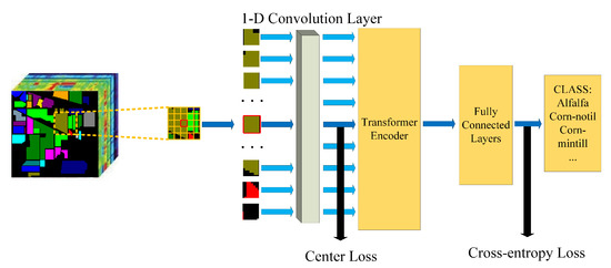
Figure 1.
The overall architecture of our proposed model.
2.1. Projection Layer with Metric Learning
We use the 1-D convolution layer as the projection layer. The 1-D convolution is calculated by convolving a 1-D kernel with the 1-D-data. The computation complexity of the 1-D convolution layer is drastically lower than the 2-D and 3-D convolution layers. It leads to a significant advantage of running time for 1-D convolution layers over 2-D and 3-D convolution layers. The computational process is presented in Figure 2. In 1-D convolution, the activation value at spatial position x in the jth feature map of the ith layer, denoted as , is generated using Equation (1) [23].
where b is the bias, m denotes the feature cube connected to the current feature cube in the th layer, W is the rth value of the kernel connected to the mth feature cube in the prior layer, and R denotes the length of the convolution kernel size.
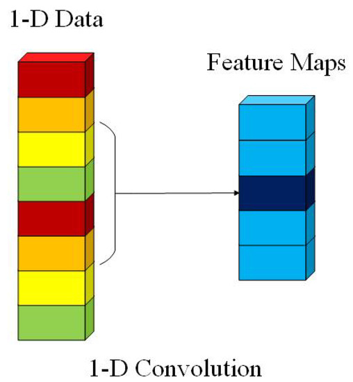
Figure 2.
The computational process of 1-D convolution.
In our model, the input image is split into 25 patches. So, we apply 25 projection layers. In order to make the model perform better, we adopt two techniques, parameter sharing, and metric learning. In our proposed model, the parameter sharing strategy can accelerate the model convergence rate and promote the classification accuracy.
The metric learning can enhance the discriminative power of the model by decreasing the intraclass distances and increasing the interclass distances. The metric learning loss term that we use in our experiment is the center loss [24], formulated as:
where x denotes the learned embedding of the ith input central patch in the batch, for i = 1, ⋯, M, and c is the kth class center based on the embeddings in kth class, for k = 1, ⋯, K.
2.2. Transformer Encoder
The transformer network was proposed in Vaswani et al. [20]. It is composed of several identical layers. Each layer was made up of two sub-layers, the multi-head self-attention mechanism and the fully connected feed-forward network, as shown in Figure 3. A residual connection followed by layer normalization is employed in each sub-layer. So, the output of each sub-layer can be defined as LayerNorm(x + SubLayer(x)), where SubLayer(x) denotes the function implemented by the sub-layer. The multi-head self-attention is defined as:
where head Attention , , , and are parameter matrices. The attention is formulated as:
where Q, K of dimension , and V of dimension are three defined learnable weight matrices.
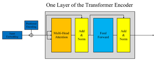
Figure 3.
The architecture of the transformer encoder.
2.3. Fully Connected Layers
The fully connected layers consist of a layernorm layer, two fully connected layers, and the Mish activation function. The Mish function is defined as
where x is the input of the function. The difference between Mish and Relu is shown in Figure 4. The benefit of Mish will be proved in the next section.
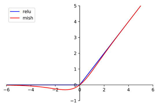
Figure 4.
The difference between Mish and Relu.
3. Experiment
3.1. Data Set Description and Training Details
We evaluate the proposed model on three publicly available hyperspectral image data sets, namely Indian Pines, University of Pavia, and Salinas, as illustrated in Figure 5, Figure 6 and Figure 7. The spectral radiance of these three data sets and the corresponding categories are shown in Figure 8, Figure 9, Figure 10 and Figure 11.
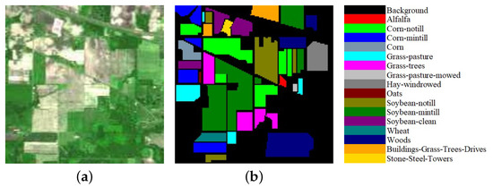
Figure 5.
(a) False-color Indian Pines image. (b) Ground-truth map of the Indian Pines data set.
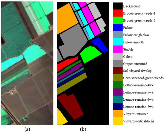
Figure 6.
(a) False-color Salinas image. (b) Ground-truth map of the Salinas data set.
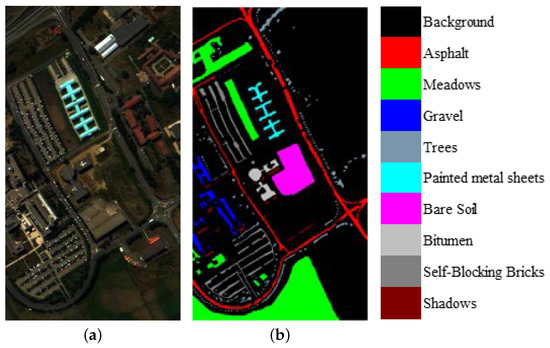
Figure 7.
(a) False-color University of Pavia image. (b) Ground-truth map of the University of Pavia data set.
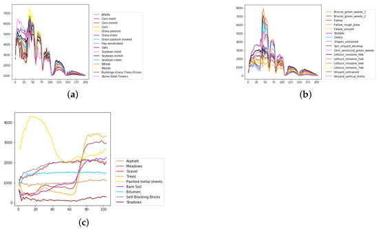
Figure 8.
The overall spectral radiance and the corresponding categories in different data sets. (a) Indian Pines. (b) Salinas. (c) University of Pavia.

Figure 9.
The spectral radiance of different pixels and the corresponding categories in Indian Pines. (a) Alfalfa. (b) Corn-notill. (c) Corn-mintill. (d) Corn. (e) Grass-pasture. (f) Grass-trees. (g) Grass-pasture-mowed. (h) Hay-windrowed. (i) Oats. (j) Soybean-notill. (k) Soybean-mintill. (l) Soybean-clean. (m) Wheat. (n) Woods. (o) Buildings-Grass-Trees-Drives. (p) Stone-Steel-Towers.

Figure 10.
The spectral radiance of different pixels and the corresponding categories in Salinas. (a) Brocoli_green_weeds_1. (b) Brocoli_green_weeds_2. (c) Fallow. (d) Fallow_rough_plow. (e) Fallow_smooth. (f) Stubble. (g) Celery. (h) Grapes_untrained. (i) Soil_vinyard_develop. (j) Corn_senesced_green_weeds. (k) Lettuce_romaine_4wk. (l) Lettuce_romaine_5wk. (m) Lettuce_romaine_6wk. (n) Lettuce_romaine_7wk. (o) Vinyard_untrained. (p) Vinyard_vertical_trellis.
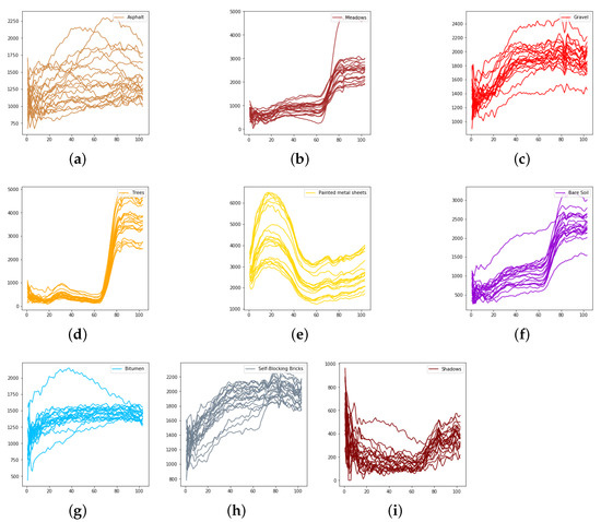
Figure 11.
The spectral radiance of different pixels and the corresponding categories in the University of Pavia. (a) Asphalt. (b) Meadows. (c) Gravel. (d) Trees. (e) Painted metal sheets. (f) Bare Soil. (g) Bitumen. (h) Self-Blocking Bricks. (i) Shadows.
The Indian Pines data set was collected by the Airborne Visible/Infrared Imaging Spectrometer (AVIRIS) from Northwestern Indiana. The scene contains 145 pixels with a spatial resolution of 20 m by pixel and 224 spectral channels in the wavelength range from 0.4 to 2.5 m. After 24 bands corrupted by water absorption effects were removed, 200 bands were available for analysis and experiments. The 10,249 labeled pixels were divided into 16 classes.
The University of Pavia data set was acquired by the Reflective Optics System Imaging Spectrometer (ROSIS) over Pavia, northern Italy. The image size was 610 with a spatial resolution of 1.3 m by pixel and 103 spectral bands in the wavelength range from 0.43 to 0.86 m. The 42,776 labeled pixels were designed into 9 categories.
The Salinas data set was gathered by the AVIRIS sensor over Salinas Valley, California. The image contains 512 pixels with a spatial resolution of 3.7 m by pixel and 224 spectral channels in the wavelength range from 0.4 to 2.5 m. After 20 water-absorbing spectral bands were discarded, 204 bands were accessible for classification. The 54,129 labeled pixels were partitioned into 16 categories.
For the Indian Pines, the proportion of samples for training and validation was set to 3%. For the University of Pavia, we set the ratios of training samples and validation samples to 0.5%. For the Salinas, we selected 0.4% of the samples for training and 0.4% for validation. Table 1, Table 2 and Table 3 list the number of training, validation, and testing samples of the three data sets.

Table 1.
Training, validation, and testing sample numbers in Indian Pines.
Table 2.
Training, validation, and testing sample numbers in Salinas.
Table 3.
Training, validation, and testing sample numbers in the University of Pavia.
All experiments were conducted using the same device with the RTX Titan GPU and 16 GB RAM. The learning rate was set to 0.0005, and the number of epochs was 200. The model with the least cross-entropy loss in the validation samples was selected for testing. We used mini-batches with a size of 256 for all experiments. The weight of the metric learning loss term was set to 10. We apply the traditional principal component analysis (PCA) over the original HSI data to remove the spectral redundancy. To compare the performances of experimental models fairly, we use the same input size over each data set, such as 25 × 25 × 30 for the Indian Pines and 25 × 25 × 15 for the University of Pavia and the Salinas, respectively. In order to ensure the accuracy and stability of the experimental results, we conducted the experiments 10 times consecutively. The parameter summary of the proposed transformer model architecture over the three data sets is shown in Table 4, Table 5, Table 6 and Table 7.
Table 4.
Configuration of our proposed model variants.
Table 5.
Parameter summary of the proposed transformer model architecture over the Indian Pines data set.
Table 6.
Parameter summary of the proposed transformer model architecture over the Salinas data set.
Table 7.
Parameter summary of the proposed transformer model architecture over the University of Pavia data set.
3.2. Classification Results
To evaluate the performance of the proposed method, we used three metrics: overall accuracy (OA), average accuracy (AA), and the Kappa coefficient (Kappa). OA is the percentage of correctly classified samples over the total test samples. AA is the average accuracy from each class, and Kappa measures the consistency between the predicted result and ground truth. The results of the proposed transformer model are compared with traditional deep-learning methods, such as 2-D-CNN [25], 3-D-CNN [26], Multi-3-D CNN [27], and hybridSN [17].
Table 8, Table 9 and Table 10 show the categorized results using different methods. The numbers after the plus-minus signs are the variances of the corresponding metrics. Figure 12, Figure 13 and Figure 14 demonstrate classification maps for each of the methods. The preliminary analysis of the results revealed that our proposed model could provide a more accurate classification result than other models over each data set. Among the contrast models, the OA, AA, and Kappa of HybridSN were higher than those of other contrast models. It indicates that the 3-D-2-D-CNN models were more suitable for the hyperspectral image classification with limited training samples than the models that used 2-D convolution or 3-D convolution alone. Secondly, it can be observed from these results that the performance of 2-D-CNN was better than that of 3-D-CNN or Multi-3-D-CNN. To the best of our knowledge, it was probably because the large parameter size can easily lead to overfitting when the training samples were lacking.
Table 8.
Classification results of different models in Indian Pines.
Table 9.
Classification results of different models in Salinas.
Table 10.
Classification results of different models in the University of Pavia.
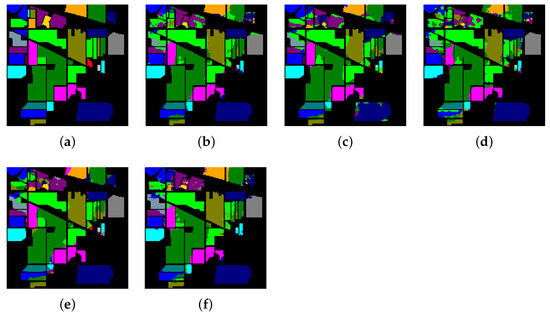
Figure 12.
The classification maps of Indian Pines. (a) Ground-truth map. (b)–(f) Classification results of 2-D-convolutional neural network (CNN), 3-D-CNN, Multi-3-D-CNN, HybridSN, and Transformer.

Figure 13.
The classification maps of Salinas. (a) Ground-truth map. (b)–(f) Classification results of 2-D-CNN, 3-D-CNN, Multi-3-D-CNN, HybridSN, and Transformer.

Figure 14.
The classification maps of the University of Pavia. (a) Ground-truth map. (b)–(f) Classification results of 2-D-CNN, 3-D-CNN, Multi-3-D-CNN, HybridSN, and Transformer.
Considering the spectral information, we can conclude that the spectral information can influence the classification accuracy greatly. For example, in Indian Pines, the spectral feature of Grass-pasture-mowed is significantly different from the features of the other classes over the first 75 spectral bands. Besides, the pixels of Grass-pasture-mowed have similar spectral features. Although we only used one sample of Grass-pasture-mowed for training. All the models can reach the accuracy of at least 85%.
Table 11 summarizes the parameter size of the five models. The two rows of each model are the number of parameters and the memory space occupied by the parameters. It is apparent from this table that the transformer model was of the smallest parameter size, indicating the efficiency of the transformer model.
Table 11.
Parameter size of the five methods on the three hyperspectral data sets.
Table 12 shows the floating-point operations (flops) of the five models. Table 13, Table 14 and Table 15 compare the training time and testing time of the five models over each data set. The computational costs of our proposed model were the least. Because of the GPU acceleration for convolutions, the 2-D-CNN was quicker than our proposed model. Considering that the accuracy of the 2-D-CNN was lower than that of our proposed model, we think our method has a better balance of accuracy and efficiency.
Table 12.
Flops of the five methods on the three hyperspectral data sets.
Table 13.
Running time of the five methods on the Indian Pines data set.
Table 14.
Running time of the five methods on the Salinas data set.
Table 15.
Running time of the five methods on the University of Pavia data set.
4. Discussion
In this part, further analysis of our proposed model is provided. Firstly, metric learning can improve the model classification performance significantly, especially when the training samples are extremely lacking, and the results prove it. Secondly, the results of controlled experiments reflect the benefits of 1-D convolution layers with parameter sharing. Thirdly, the experimental results about different activation functions confirm the superiority of Mish.
4.1. Effectiveness of the Metric Learning
To prove the effectiveness of the metric learning, we remove the metric learning mechanism and compare the performance between these two models.
Table 16 and Figure 15, Figure 16 and Figure 17 reveal the benefits of the metric learning mechanism. The numbers after the plus-minus signs are the variances of the corresponding metrics. The model with metric learning can reach a higher accuracy. We can conclude that the metric learning can improve the model classification results.
Table 16.
Classification results of the transformer without metric learning and the transformer with metric learning.
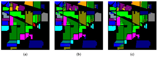
Figure 15.
The classification maps of Indian Pines. (a) Ground-truth map. (b) Classification results of the Transformer without metric learning. (c) Classification results of the Transformer with metric learning.
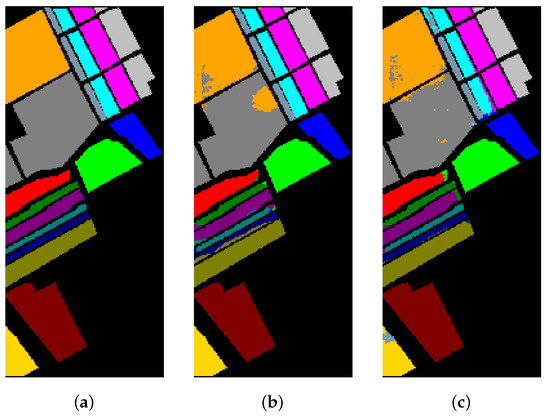
Figure 16.
The classification maps of Salinas. (a) Ground-truth map. (b) Classification results of the Transformer without metric learning. (c) Classification results of the Transformer with metric learning.
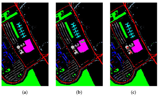
Figure 17.
The classification maps of University of Pavia. (a) Ground-truth map. (b) Classification results of the Transformer without metric learning. (c) Classification results of the Transformer with metric learning.
4.2. Effectiveness of the 1-D Convolution and Parameter Sharing
In Section 2.1, we declare that the parameter sharing strategy can improve the model classification result. Here, we will compare the performance of the transformer model with the 1-D convolution and parameter sharing, the transformer model with 1-D convolution, the transformer model with the linear projection layers and parameter sharing, and the transformer model with the linear projection layers.
From Figure 18, we can conclude that both 1-D convolution layers and parameter sharing boost the model performance.
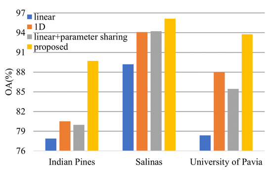
Figure 18.
Effectiveness of the 1-D convolution and parameter sharing.
4.3. Effectiveness of the Activation Function
The Mish activation function can promote model performance slightly. Figure 19 shows the classification OA of the transformer models based on different activation functions.
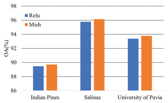
Figure 19.
Effectiveness of the activation function.
5. Conclusions
In this article, we introduce the transformer architecture for hyperspectral image classification. Meanwhile, by replacing the linear projection layer with the 1-D convolution layer, the image patches can be embedded into sequences with more information. It can lead to an increase in classification accuracy. Besides, the Mish activation function is adopted instead of the Relu activation function; hence, the model performance can be further boosted.
In the experiments, the influence of three innovative changes based on the classical vision transformer, including metric learning, the 1-D convolution layer, and the Mish activation function, is proved. Moreover, many state-of-the-art methods based on convolutional neural networks, including 2-D CNN, 3-D CNN, multi-scale 3-D CNN, and hybrid CNN, are taken into account. The results demonstrate the advantage of the proposed model, especially under the condition of lacking training samples.
Author Contributions
X.H. and H.W. implement the algorithms, designing the experiments, and wrote the paper; Y.L. performed the experiments; Y.P. and W.Y. guided the research. All authors have read and agreed to the published version of the manuscript.
Funding
This research was partially supported by the National Key Research and Development Program of China (No.2017YFB1301104 and 2017YFB1001900), and the National Natural Science Foundation of China (No.91648204 and 61803375), and the National Science and Technology Major Project.
Institutional Review Board Statement
Not applicable.
Informed Consent Statement
Not applicable.
Data Availability Statement
The datasets involved in this paper are all public datasets.
Acknowledgments
The authors acknowledge the State Key Laboratory of High-Performance Computing, College of Computer, National University of Defense Technology, China.
Conflicts of Interest
The authors declare no conflict of interest.
Abbreviations
The following abbreviations are used in this manuscript:
| HSI | Hyperspectral Image |
| CNN | Convolutional Neural Network |
| GPU | Graphics Processing Unit |
| DL | Deep Learning |
| RAE | Recursive Autoencoder |
| DBN | Deep Belief Network |
| RBM | Boltzmann Machine |
| DML | Deep Metric Learning |
| NLP | Natural Language Processing |
References
- Marinelli, D.; Bovolo, F.; Bruzzone, L. A novel change detection method for multitemporal hyperspectral images based on a discrete representation of the change information. In Proceedings of the 2017 IEEE International Geoscience and Remote Sensing Symposium (IGARSS), Fort Worth, TX, USA, 23–28 July 2017; pp. 161–164. [Google Scholar]
- Liang, H.; Li, Q. Hyperspectral imagery classification using sparse representations of convolutional neural network features. Remote Sens. 2016, 8, 99. [Google Scholar] [CrossRef]
- Sun, W.; Yang, G.; Du, B.; Zhang, L.; Zhang, L. A sparse and low-rank near-isometric linear embedding method for feature extraction in hyperspectral imagery classification. IEEE Trans. Geosci. Remote. Sens. 2017, 55, 4032–4046. [Google Scholar] [CrossRef]
- Awad, M. Sea water chlorophyll-a estimation using hyperspectral images and supervised artificial neural network. Ecol. Inform. 2014, 24, 60–68. [Google Scholar] [CrossRef]
- He, K.; Zhang, X.; Ren, S.; Sun, J. Deep residual learning for image recognition. In Proceedings of the IEEE Conference on Computer Vision and Pattern Recognition, Las Vegas, NV, USA, 26 June–1 July 2016; pp. 770–778. [Google Scholar]
- Durand, T.; Mehrasa, N.; Mori, G. Learning a deep convnet for multi-label classification with partial labels. In Proceedings of the IEEE Conference on Computer Vision and Pattern Recognition, Long Beach, CA, USA, 16–20 June 2019; pp. 647–657. [Google Scholar]
- Liu, Y.; Dou, Y.; Jin, R.; Li, R.; Qiao, P. Hierarchical learning with backtracking algorithm based on the visual confusion label tree for large-scale image classification. Vis. Comput. 2021, 1–21. [Google Scholar] [CrossRef]
- Liu, Y.; Dou, Y.; Jin, R.; Qiao, P. Visual tree convolutional neural network in image classification. In Proceedings of the 2018 24th International Conference on Pattern Recognition (ICPR), Beijing, China, 20–24 August 2018; pp. 758–763. [Google Scholar]
- Ren, S.; He, K.; Girshick, R.; Sun, J. Faster r-cnn: Towards real-time object detection with region proposal networks. IEEE Trans. Pattern Anal. Mach. Intell. 2016, 39, 1137–1149. [Google Scholar] [CrossRef] [PubMed]
- He, K.; Gkioxari, G.; Dollár, P.; Girshick, R. Mask r-cnn. In Proceedings of the IEEE International Conference on Computer Vision, Venice, Italy, 22–29 October 2017; pp. 2961–2969. [Google Scholar]
- Nagpal, C.; Dubey, S.R. A performance evaluation of convolutional neural networks for face anti spoofing. In Proceedings of the 2019 International Joint Conference on Neural Networks (IJCNN), Budapest, Hungary, 14–19 July 2019; pp. 1–8. [Google Scholar]
- Chen, Y.; Lin, Z.; Zhao, X.; Wang, G.; Gu, Y. Deep learning-based classification of hyperspectral data. IEEE J. Sel. Top. Appl. Earth Obs. Remote. Sens. 2014, 7, 2094–2107. [Google Scholar] [CrossRef]
- Ma, X.; Wang, H.; Geng, J. Spectral–spatial classification of hyperspectral image based on deep auto-encoder. IEEE J. Sel. Top. Appl. Earth Obs. Remote. Sens. 2016, 9, 4073–4085. [Google Scholar] [CrossRef]
- Zhang, X.; Liang, Y.; Li, C.; Huyan, N.; Jiao, L.; Zhou, H. Recursive autoencoders-based unsupervised feature learning for hyperspectral image classification. IEEE Geosci. Remote. Sens. Lett. 2017, 14, 1928–1932. [Google Scholar] [CrossRef]
- Chen, Y.; Zhao, X.; Jia, X. Spectral–spatial classification of hyperspectral data based on deep belief network. IEEE J. Sel. Top. Appl. Earth Obs. Remote. Sens. 2015, 8, 2381–2392. [Google Scholar] [CrossRef]
- Chen, Y.; Jiang, H.; Li, C.; Jia, X.; Ghamisi, P. Deep feature extraction and classification of hyperspectral images based on convolutional neural networks. IEEE Trans. Geosci. Remote. Sens. 2016, 54, 6232–6251. [Google Scholar] [CrossRef]
- Roy, S.K.; Krishna, G.; Dubey, S.R.; Chaudhuri, B.B. Hybridsn: Exploring 3-d–2-d cnn feature hierarchy for hyperspectral image classification. IEEE Geosci. Remote. Sens. Lett. 2019, 17, 277–281. [Google Scholar] [CrossRef]
- Cheng, G.; Yang, C.; Yao, X.; Guo, L.; Han, J. When deep learning meets metric learning: Remote sensing image scene classification via learning discriminative cnns. IEEE Trans. Geosci. Remote. Sens. 2018, 56, 2811–2821. [Google Scholar] [CrossRef]
- Guo, A.J.; Zhu, F. Spectral-spatial feature extraction and classification by ann supervised with center loss in hyperspectral imagery. IEEE Trans. Geosci. Remote. Sens. 2018, 57, 1755–1767. [Google Scholar] [CrossRef]
- Vaswani, A.; Shazeer, N.; Parmar, N.; Uszkoreit, J.; Jones, L.; Gomez, A.N.; Kaiser, L.; Polosukhin, I. Attention is all you need. Adv. Neural Inf. Process. Syst. 2017, 30, 5998–6008. [Google Scholar]
- Dosovitskiy, A.; Beyer, L.; Kolesnikov, A.; Weissenborn, D.; Zhai, X.; Unterthiner, T.; Dehghani, M.; Minderer, M.; Heigold, G.; Gelly, S.; et al. An image is worth 16x16 words: Transformers for image recognition at scale. arXiv 2020, arXiv:2010.11929. [Google Scholar]
- Misra, D. Mish: A self regularized non-monotonic neural activation function. arXiv 2019, arXiv:1908.08681. [Google Scholar]
- Kiranyaz, S.; Avci, O.; Abdeljaber, O.; Ince, T.; Gabbouj, M.; Inman, D.J. 1d convolutional neural networks and applications: A survey. arXiv 2019, arXiv:1905.03554. [Google Scholar] [CrossRef]
- Wen, Y.; Zhang, K.; Li, Z.; Qiao, Y. A discriminative feature learning approach for deep face recognition. In Proceedings of the European Conference on Computer Vision, Amsterdam, The Netherlands, 11–14 October 2016; pp. 499–515. [Google Scholar]
- Liu, B.; Yu, X.; Zhang, P.; Tan, X.; Yu, A.; Xue, Z. A semi-supervised convolutional neural network for hyperspectral image classification. Remote. Sens. Lett. 2017, 8, 839–848. [Google Scholar] [CrossRef]
- Hamida, A.B.; Benoit, A.; Lambert, P.; Amar, C.B. 3-d deep learning approach for remote sensing image classification. IEEE Trans. Geosci. Remote. Sens. 2018, 56, 4420–4434. [Google Scholar] [CrossRef]
- He, M.; Li, B.; Chen, H. Multi-scale 3d deep convolutional neural network for hyperspectral image classification. In Proceedings of the 2017 IEEE International Conference on Image Processing (ICIP), Beijing, China, 17–20 September 2017; pp. 3904–3908. [Google Scholar]


Publisher’s Note: MDPI stays neutral with regard to jurisdictional claims in published maps and institutional affiliations. |
© 2021 by the authors. Licensee MDPI, Basel, Switzerland. This article is an open access article distributed under the terms and conditions of the Creative Commons Attribution (CC BY) license (http://creativecommons.org/licenses/by/4.0/).