
Practices and Applications of Convolutional Neural Network-Based Computer Vision Systems in Animal Farming: A Review

 ,
, 
 ,
, 
Abstract
1. Introduction
2. Study Background
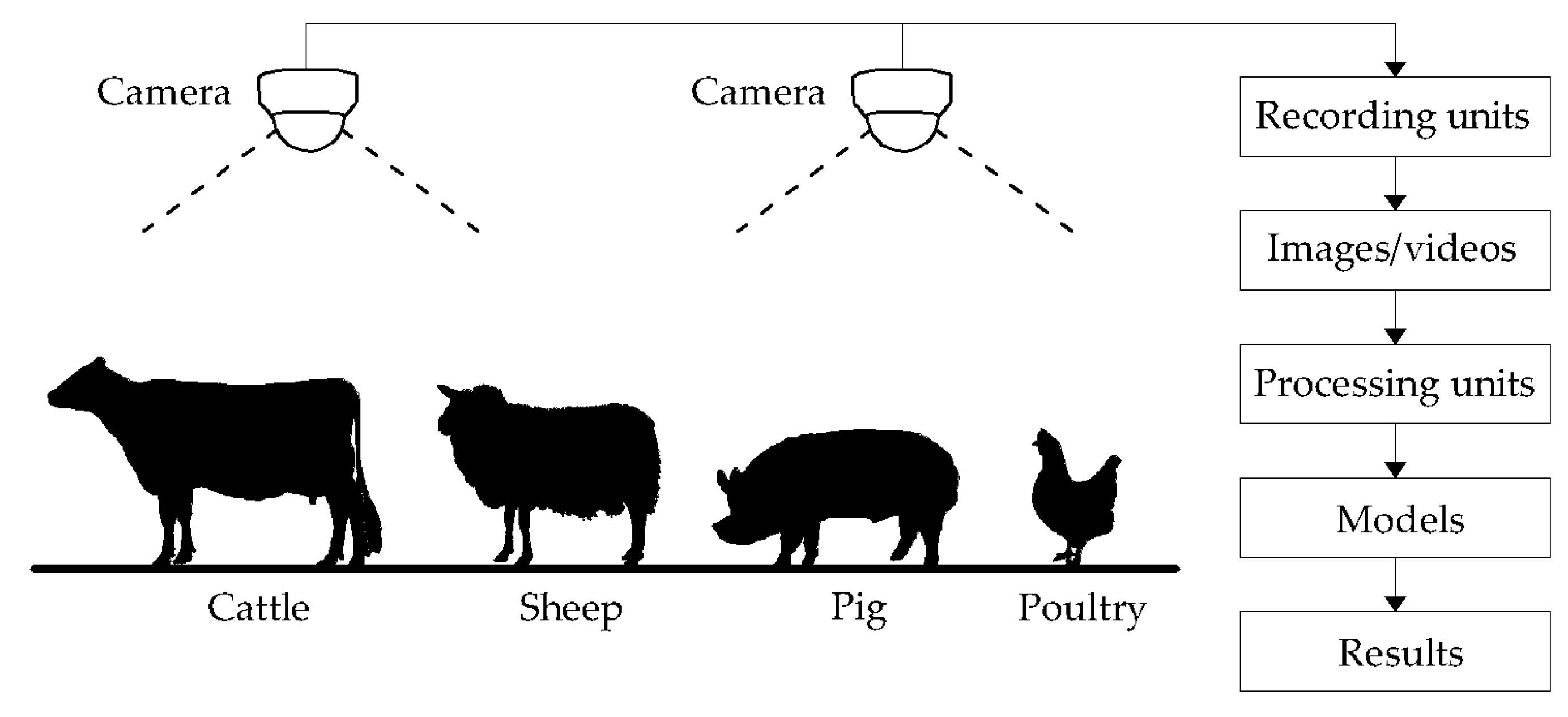
2.1. Definition of Farm Animals
- Cattle: a common type of large, domesticated, ruminant animals. In this case, they include dairy cows farmed for milk and beef cattle farmed for meat.
- Pig: a common type of large, domesticated, even-toed animals. In this case, they are sow farmed for reproducing piglets, piglet (a baby or young pig before it is weaned), and swine (alternatively termed pig) farmed for meat.
- Ovine: a common type of large, domesticated, ruminant animals. In this case, they are sheep (grazer) farmed for meat, fiber (wool), and sometimes milk, lamb (a young sheep), and goat (browser) farmed for meat, milk, and sometimes fiber (wool).
- Poultry: a common type of small, domesticated, oviparous animals. In this case, they are broiler farmed for meat, laying hen farmed for eggs, breeder farmed for reproducing fertilized eggs, and pullet (a young hen).
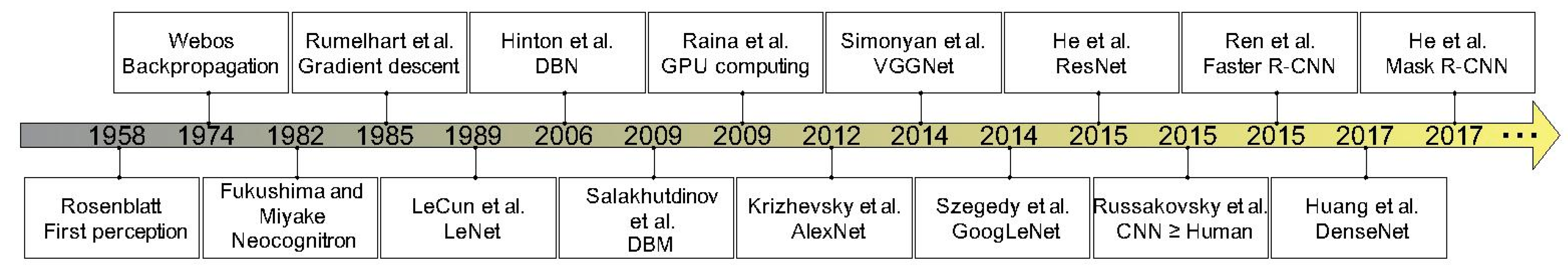
2.2. History of Artificial Neural Networks for Convolutional Neural Networks in Evaluating Images/Videos
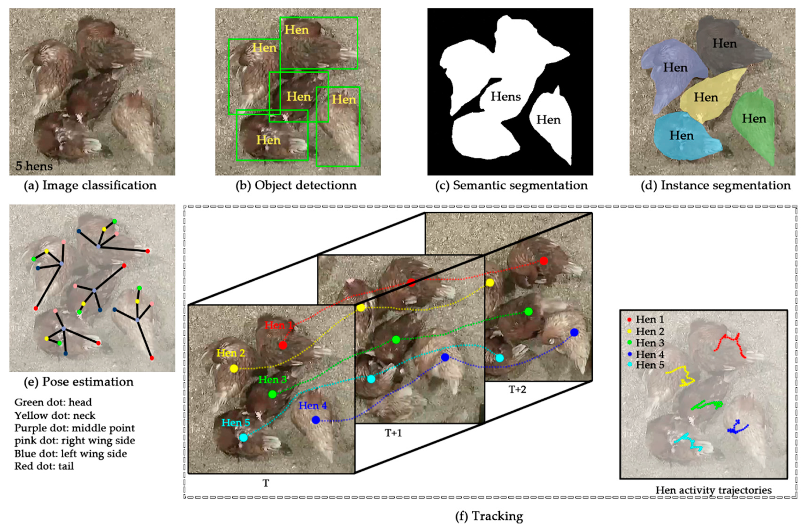
2.3. Computer Vision Tasks
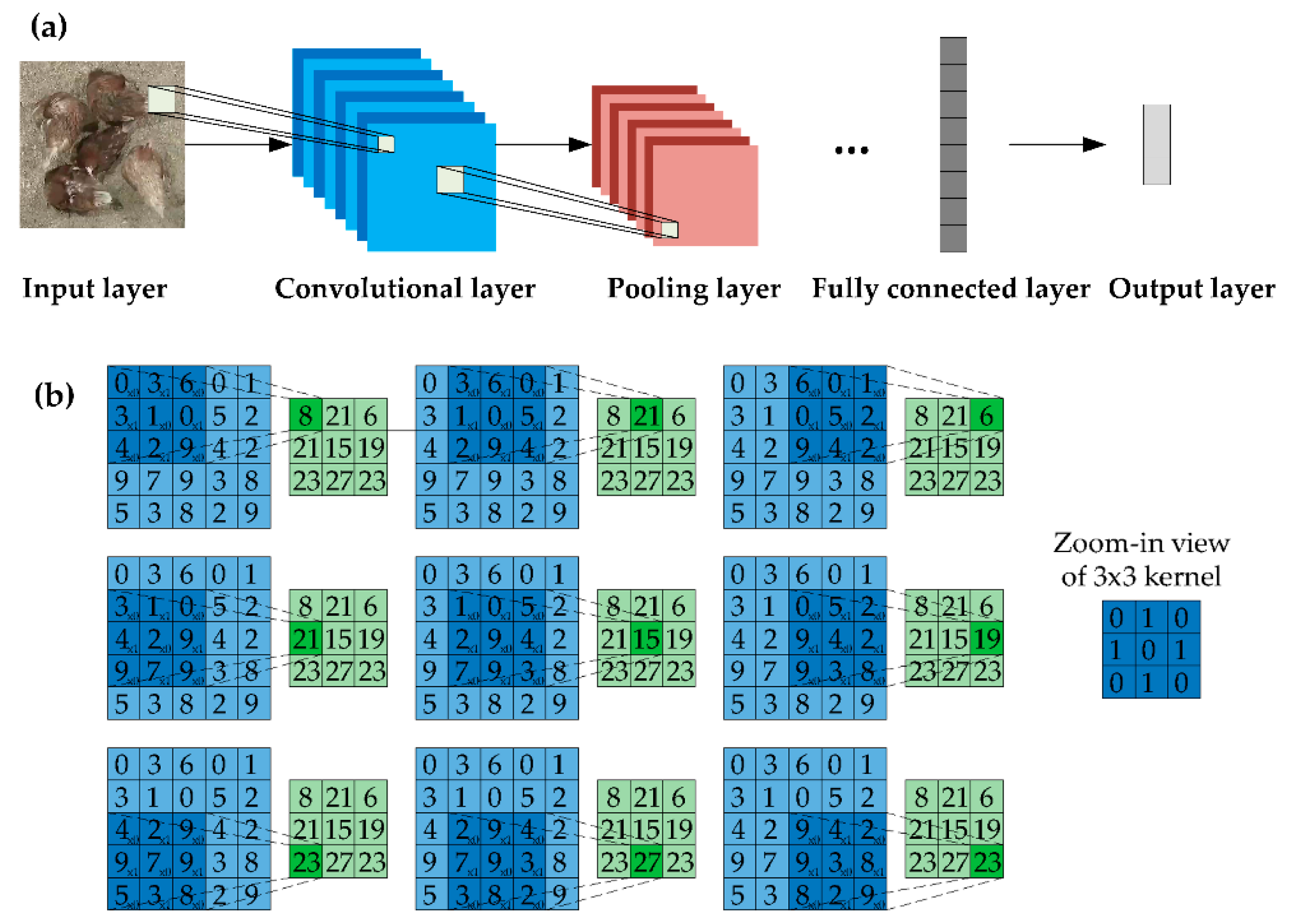
2.4. “Convolutional Neural Network-Based” Architecture
2.5. Literature Search Term and Search Strategy
3. Preparations
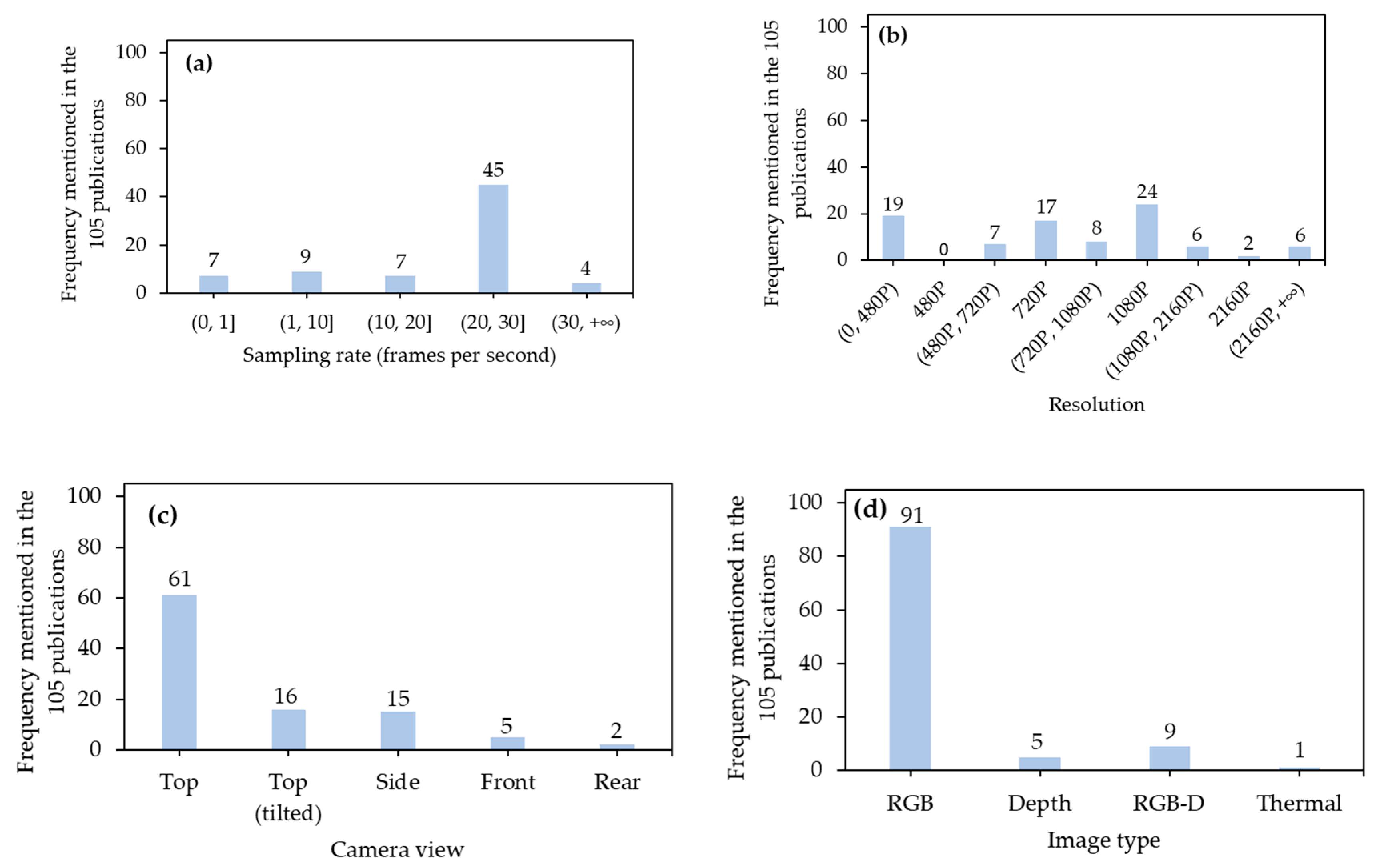
3.1. Camera Setups
3.1.1. Sampling Rate
3.1.2. Resolution
3.1.3. Camera View
3.1.4. Image Type
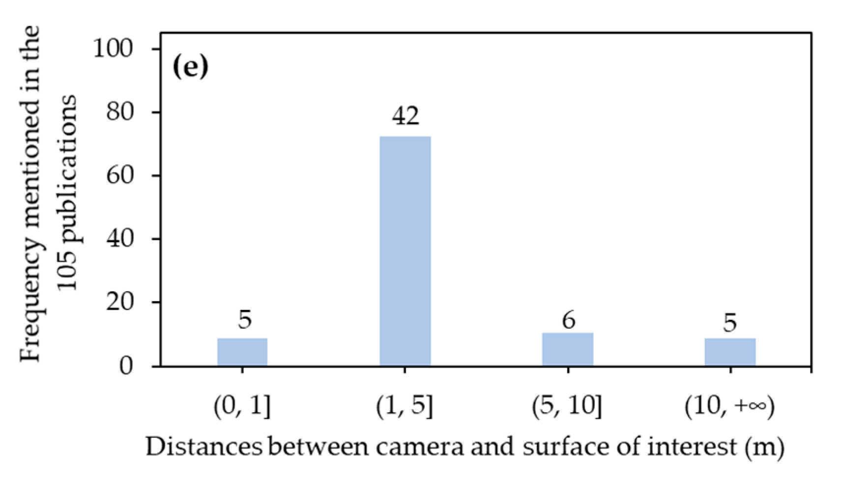
3.1.5. Distance between Camera and Surface of Interest
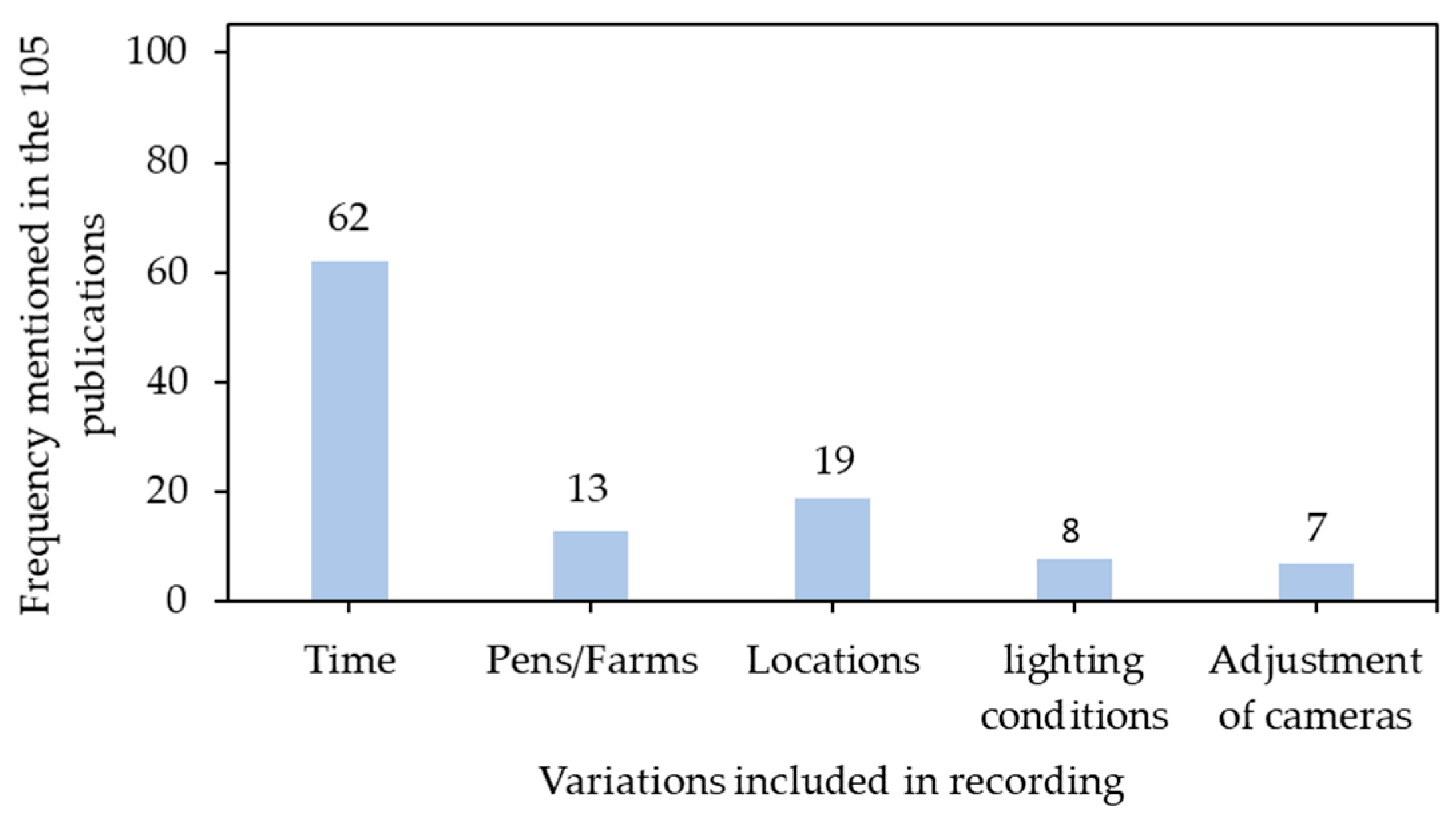
3.2. Inclusion of Variations in Data Recording
3.3. Selection of Graphics Processing Units
3.4. Image Preprocessing
3.4.1. Selection of Key Frames
3.4.2. Class Balance in Dataset
3.4.3. Adjustment of Image Channels
3.4.4. Image Cropping
3.4.5. Image Enhancement
3.4.6. Image Restoration
3.4.7. Image Segmentation
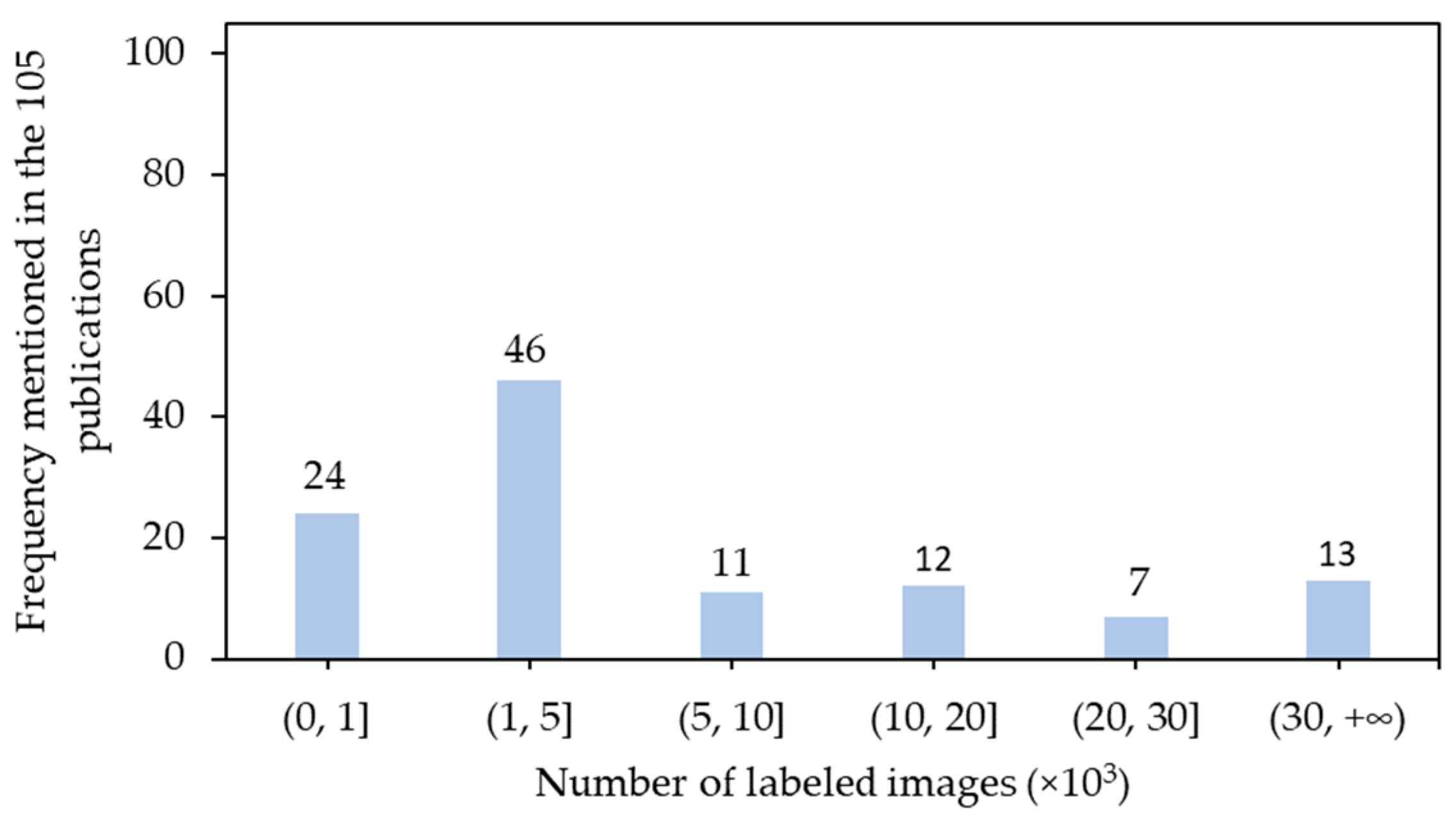
3.5. Data Labeling
4. Convolutional Neural Network Architectures
4.1. Architectures for Image Classification
4.2. Architectures for Object Detection
4.3. Architectures for Semantic/Instance Segmentation
4.4. Architectures for Pose Estimation
4.5. Architectures for Tracking
5. Strategies for Algorithm Development
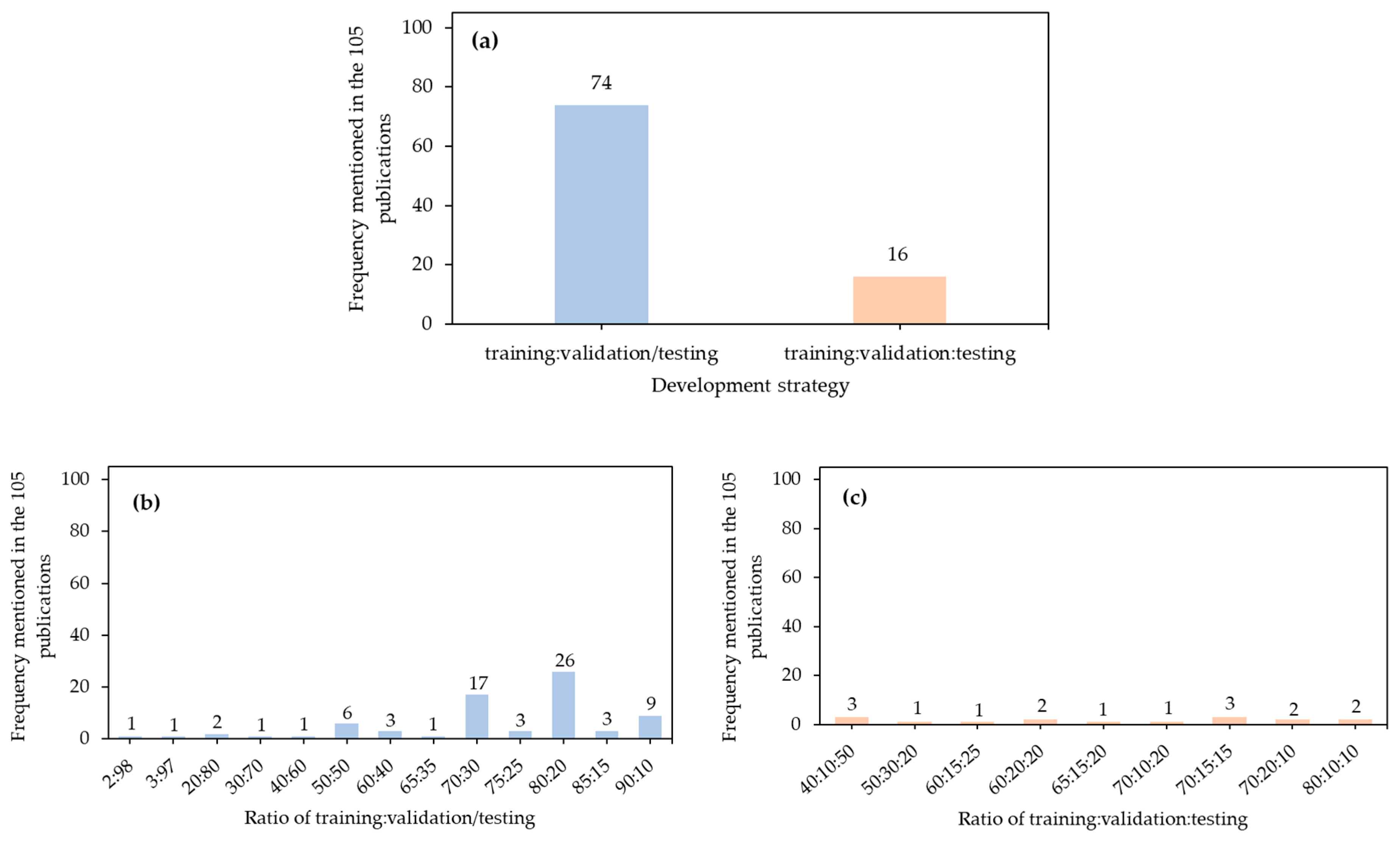
5.1. Distribution of Development Data
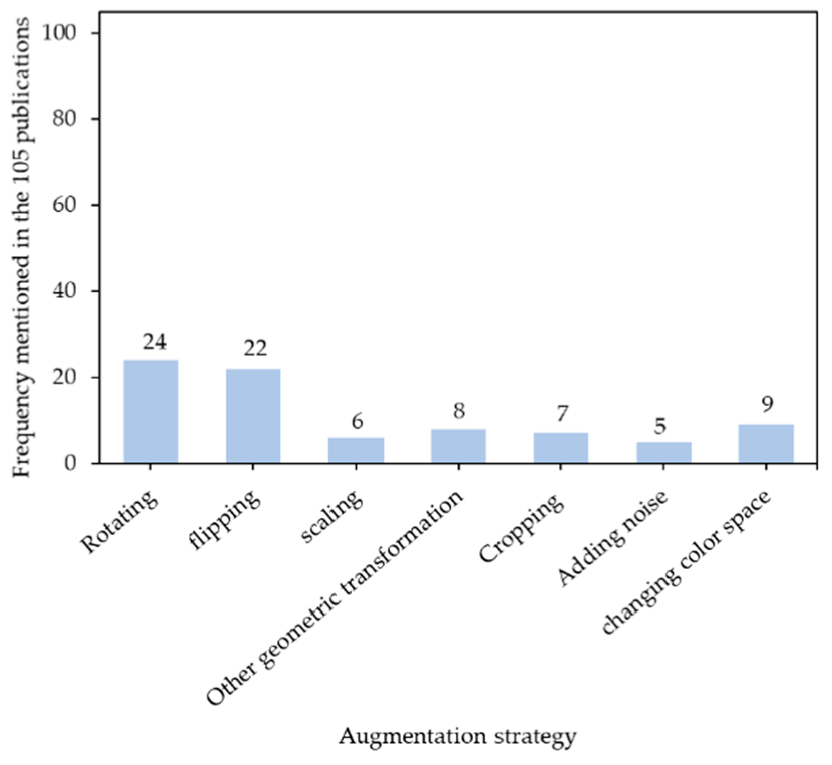
5.2. Data Augmentation
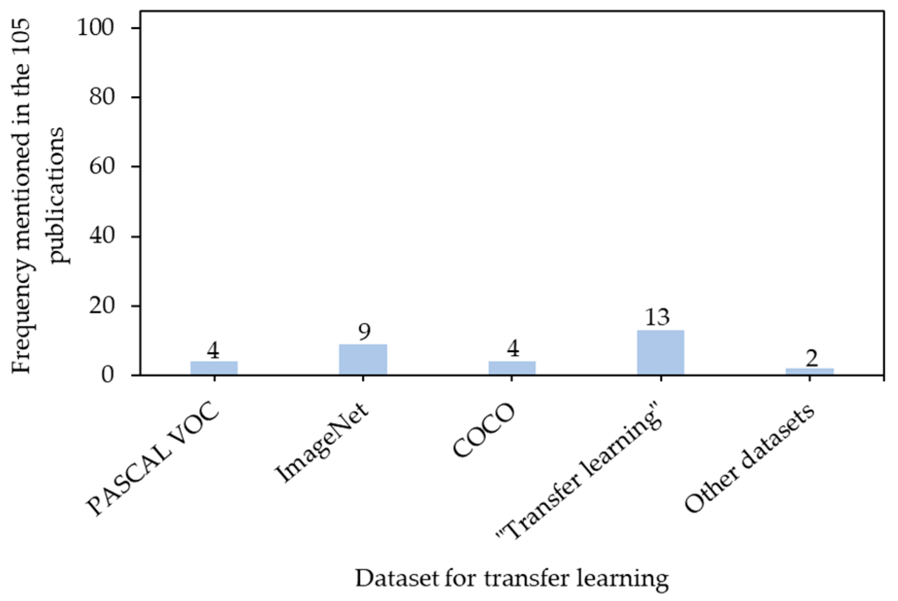
5.3. Transfer Learning
5.4. Hyperparameters
5.4.1. Gradient Descent Mode
5.4.2. Learning Rate
5.4.3. Batch Size
5.4.4. Optimizer of Training
5.4.5. Regularization
5.4.6. Hyperparameters Tuning
5.5. Evaluation Metrics
6. Performance
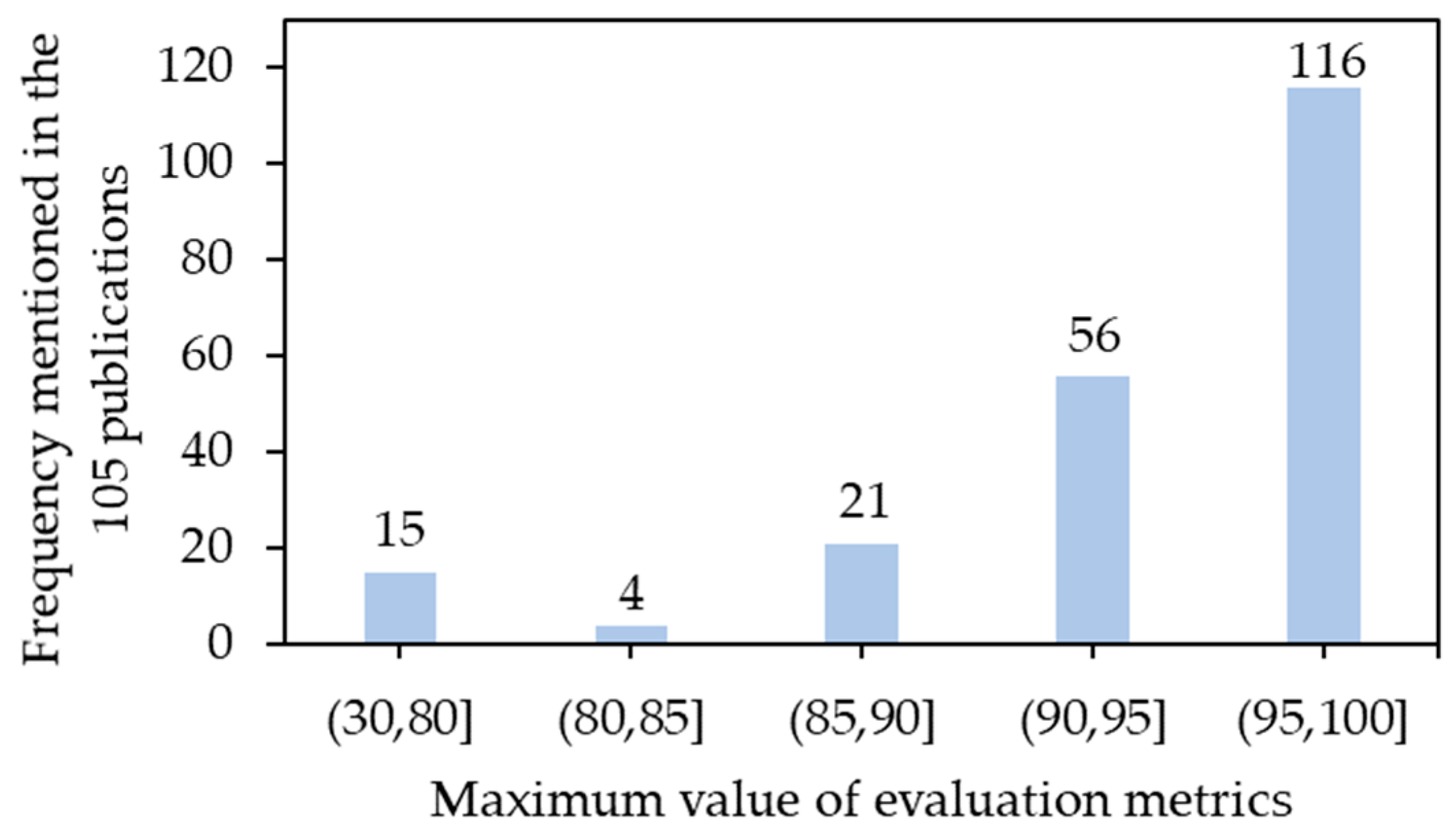
6.1. Performance Judgment
6.2. Architecture Performance
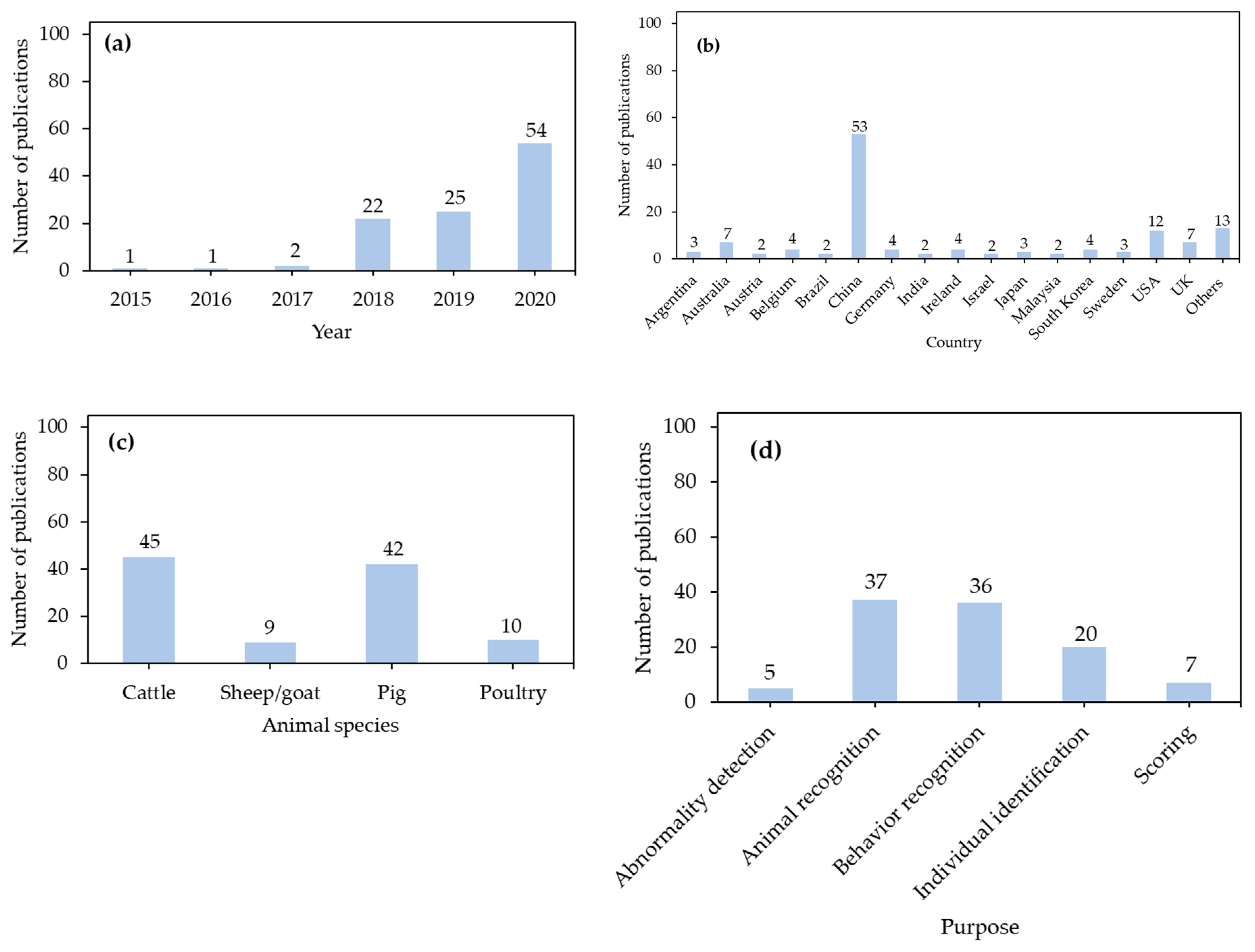
7. Applications
7.1. Number of Publications Based on Years
7.2. Number of Publications Based on Countries
7.3. Number of Publications Based on Animal Species
7.4. Number of Publications Based on Purposes
8. Brief Discussion and Future Directions
8.1. Movable Solutions
8.2. Availability of Datasets
8.3. Research Focuses
8.4. Multidisciplinary Cooperation
9. Conclusions
Author Contributions
Funding
Institutional Review Board Statement
Informed Consent Statement
Data Availability Statement
Conflicts of Interest
References
- Tilman, D.; Balzer, C.; Hill, J.; Befort, B.L. Global food demand and the sustainable intensification of agriculture. Proc. Natl. Acad. Sci. USA 2011, 108, 20260–20264. [Google Scholar] [CrossRef] [PubMed]
- McLeod, A. World Livestock 2011-Livestock in Food Security; Food and Agriculture Organization of the United Nations (FAO): Rome, Italy, 2011. [Google Scholar]
- Yitbarek, M. Livestock and livestock product trends by 2050: A review. Int. J. Anim. Res. 2019, 4, 30. [Google Scholar]
- Beaver, A.; Proudfoot, K.L.; von Keyserlingk, M.A. Symposium review: Considerations for the future of dairy cattle housing: An animal welfare perspective. J. Dairy Sci. 2020, 103, 5746–5758. [Google Scholar] [CrossRef]
- Hertz, T.; Zahniser, S. Is there a farm labor shortage? Am. J. Agric. Econ. 2013, 95, 476–481. [Google Scholar] [CrossRef]
- Kashiha, M.; Pluk, A.; Bahr, C.; Vranken, E.; Berckmans, D. Development of an early warning system for a broiler house using computer vision. Biosyst. Eng. 2013, 116, 36–45. [Google Scholar] [CrossRef]
- Werner, A.; Jarfe, A. Programme Book of the Joint Conference of ECPA-ECPLF; Wageningen Academic Publishers: Wageningen, The Netherlands, 2003. [Google Scholar]
- Norton, T.; Chen, C.; Larsen, M.L.V.; Berckmans, D. Precision livestock farming: Building ‘digital representations’ to bring the animals closer to the farmer. Animal 2019, 13, 3009–3017. [Google Scholar] [CrossRef] [PubMed]
- Banhazi, T.M.; Lehr, H.; Black, J.; Crabtree, H.; Schofield, P.; Tscharke, M.; Berckmans, D. Precision livestock farming: An international review of scientific and commercial aspects. Int. J. Agric. Biol. Eng. 2012, 5, 1–9. [Google Scholar]
- Bell, M.J.; Tzimiropoulos, G. Novel monitoring systems to obtain dairy cattle phenotypes associated with sustainable production. Front. Sustain. Food Syst. 2018, 2, 31. [Google Scholar] [CrossRef]
- Li, G.; Ji, B.; Li, B.; Shi, Z.; Zhao, Y.; Dou, Y.; Brocato, J. Assessment of layer pullet drinking behaviors under selectable light colors using convolutional neural network. Comput. Electron. Agric. 2020, 172, 105333. [Google Scholar] [CrossRef]
- Li, G.; Zhao, Y.; Purswell, J.L.; Du, Q.; Chesser, G.D., Jr.; Lowe, J.W. Analysis of feeding and drinking behaviors of group-reared broilers via image processing. Comput. Electron. Agric. 2020, 175, 105596. [Google Scholar] [CrossRef]
- Okinda, C.; Nyalala, I.; Korohou, T.; Okinda, C.; Wang, J.; Achieng, T.; Wamalwa, P.; Mang, T.; Shen, M. A review on computer vision systems in monitoring of poultry: A welfare perspective. Artif. Intell. Agric. 2020, 4, 184–208. [Google Scholar] [CrossRef]
- LeCun, Y.; Bengio, Y.; Hinton, G. Deep learning. Nature 2015, 521, 436–444. [Google Scholar] [CrossRef] [PubMed]
- Voulodimos, A.; Doulamis, N.; Doulamis, A.; Protopapadakis, E. Deep learning for computer vision: A brief review. Comput. Intell. Neurosci. 2018, 13, 1–13. [Google Scholar] [CrossRef] [PubMed]
- Garcia-Garcia, A.; Orts-Escolano, S.; Oprea, S.; Villena-Martinez, V.; Garcia-Rodriguez, J. A review on deep learning techniques applied to semantic segmentation. arXiv 2017, arXiv:1704.06857. [Google Scholar]
- Rawat, W.; Wang, Z. Deep convolutional neural networks for image classification: A comprehensive review. NeCom 2017, 29, 2352–2449. [Google Scholar] [CrossRef] [PubMed]
- Zhao, Z.-Q.; Zheng, P.; Xu, S.-t.; Wu, X. Object detection with deep learning: A review. IEEE Trans. Neural Netw. Learn. Syst. 2019, 30, 3212–3232. [Google Scholar] [CrossRef] [PubMed]
- Jiang, Y.; Li, C. Convolutional neural networks for image-based high-throughput plant phenotyping: A review. Plant Phenomics 2020, 2020, 1–22. [Google Scholar] [CrossRef] [PubMed]
- Kamilaris, A.; Prenafeta-Boldú, F.X. A review of the use of convolutional neural networks in agriculture. J. Agric. Sci. 2018, 156, 312–322. [Google Scholar] [CrossRef]
- Gikunda, P.K.; Jouandeau, N. State-of-the-art convolutional neural networks for smart farms: A review. In Proceedings of the Intelligent Computing-Proceedings of the Computing Conference, London, UK, 16–17 July 2019; pp. 763–775. [Google Scholar]
- Food and Agriculture Organization of the United States. Livestock Statistics—Concepts, Definition, and Classifications. Available online: http://www.fao.org/economic/the-statistics-division-ess/methodology/methodology-systems/livestock-statistics-concepts-definitions-and-classifications/en/ (accessed on 27 October 2020).
- Rosenblatt, F. The perceptron: A probabilistic model for information storage and organization in the brain. Psychol. Rev. 1958, 65, 386. [Google Scholar] [CrossRef] [PubMed]
- Werbos, P.J. The Roots of Backpropagation: From Ordered Derivatives to Neural Networks and Political Forecasting; John Wiley & Sons: New York, NY, USA, 1994; Volume 1. [Google Scholar]
- Rumelhart, D.E.; Hinton, G.E.; Williams, R.J. Learning Internal Representations by Error Propagation; California Univ San Diego La Jolla Inst for Cognitive Science: La Jolla, CA, USA, 1985. [Google Scholar]
- Fukushima, K.; Miyake, S. Neocognitron: A self-organizing neural network model for a mechanism of visual pattern recognition. In Competition and Cooperation in Neural Nets; Springer: Berlin/Heidelberg, Germany, 1982; pp. 267–285. [Google Scholar]
- LeCun, Y.; Boser, B.; Denker, J.S.; Henderson, D.; Howard, R.E.; Hubbard, W.; Jackel, L.D. Backpropagation applied to handwritten zip code recognition. NeCom 1989, 1, 541–551. [Google Scholar] [CrossRef]
- Boser, B.E.; Guyon, I.M.; Vapnik, V.N. A training algorithm for optimal margin classifiers. In Proceedings of the Fifth Annual Workshop on Computational Learning Theory, Pittsburgh, PA, USA, 1 July 1992; pp. 144–152. [Google Scholar]
- Hinton, G.E.; Osindero, S.; Teh, Y.-W. A fast learning algorithm for deep belief nets. NeCom 2006, 18, 1527–1554. [Google Scholar] [CrossRef] [PubMed]
- Salakhutdinov, R.; Hinton, G. Deep boltzmann machines. In Proceedings of the 12th Artificial Intelligence and Statistics, Clearwater Beach, FL, USA, 15 April 2009; pp. 448–455. [Google Scholar]
- Raina, R.; Madhavan, A.; Ng, A.Y. Large-scale deep unsupervised learning using graphics processors. In Proceedings of the 26th Annual International Conference on Machine Learning, New York, NY, USA, 14 June 2009; pp. 873–880. [Google Scholar]
- Deng, J.; Dong, W.; Socher, R.; Li, L.-J.; Li, K.; Fei-Fei, L. Imagenet: A large-scale hierarchical image database. In Proceedings of the IEEE Conference on Computer Vision and Pattern Recognition, Miami Beach, FL, USA, 20–25 June 2009; pp. 248–255. [Google Scholar]
- Krizhevsky, A.; Sutskever, I.; Hinton, G.E. Imagenet classification with deep convolutional neural networks. Adv. Neural Inf. Process. Syst. 2012, 25, 1097–1105. [Google Scholar] [CrossRef]
- Simonyan, K.; Zisserman, A. Very deep convolutional networks for large-scale image recognition. arXiv 2014, arXiv:1409.1556. [Google Scholar]
- Szegedy, C.; Liu, W.; Jia, Y.; Sermanet, P.; Reed, S.; Anguelov, D.; Erhan, D.; Vanhoucke, V.; Rabinovich, A. Going deeper with convolutions. In Proceedings of the IEEE Conference on Computer Vision and Pattern Recognition, Boston, MA, USA, 7–12 June 2015; pp. 1–9. [Google Scholar]
- He, K.; Zhang, X.; Ren, S.; Sun, J. Deep residual learning for image recognition. In Proceedings of the IEEE Conference on Computer Vision and Pattern Recognition, Las Vegas, NV, USA, 26 June–1 July 2016; pp. 770–778. [Google Scholar]
- Ren, S.; He, K.; Girshick, R.; Sun, J. Faster R-CNN: Towards real-time object detection with region proposal networks. IEEE Trans. Pattern Anal. Mach. Intell. 2016, 39, 1137–1149. [Google Scholar] [CrossRef] [PubMed]
- He, K.; Gkioxari, G.; Dollár, P.; Girshick, R. Mask R-CNN. In Proceedings of the IEEE International Conference on Computer Vision, Venice, Italy, 22–29 October 2017; pp. 2961–2969. [Google Scholar]
- Huang, G.; Liu, Z.; Van Der Maaten, L.; Weinberger, K.Q. Densely connected convolutional networks. In Proceedings of the IEEE International Conference on Computer Vision, Venice, Italy, 22–29 October 2017; pp. 4700–4708. [Google Scholar]
- Russakovsky, O.; Deng, J.; Su, H.; Krause, J.; Satheesh, S.; Ma, S.; Huang, Z.; Karpathy, A.; Khosla, A.; Bernstein, M. Imagenet large scale visual recognition challenge. Int. J. Comput. Vis. 2015, 115, 211–252. [Google Scholar] [CrossRef]
- Qiao, Y.; Su, D.; Kong, H.; Sukkarieh, S.; Lomax, S.; Clark, C. BiLSTM-based individual cattle identification for automated precision livestock farming. In Proceedings of the 16th International Conference on Automation Science and Engineering (CASE), Hong Kong, China, 20–21 August 2020; pp. 967–972. [Google Scholar]
- Psota, E.T.; Schmidt, T.; Mote, B.; C Pérez, L. Long-term tracking of group-housed livestock using keypoint detection and MAP estimation for individual animal identification. Sensors 2020, 20, 3670. [Google Scholar] [CrossRef] [PubMed]
- Bonneau, M.; Vayssade, J.-A.; Troupe, W.; Arquet, R. Outdoor animal tracking combining neural network and time-lapse cameras. Comput. Electron. Agric. 2020, 168, 105150. [Google Scholar] [CrossRef]
- Kang, X.; Zhang, X.; Liu, G. Accurate detection of lameness in dairy cattle with computer vision: A new and individualized detection strategy based on the analysis of the supporting phase. J. Dairy Sci. 2020, 103, 10628–10638. [Google Scholar] [CrossRef]
- Shao, W.; Kawakami, R.; Yoshihashi, R.; You, S.; Kawase, H.; Naemura, T. Cattle detection and counting in UAV images based on convolutional neural networks. Int. J. Remote Sens. 2020, 41, 31–52. [Google Scholar] [CrossRef]
- Tu, S.; Liu, H.; Li, J.; Huang, J.; Li, B.; Pang, J.; Xue, Y. Instance segmentation based on mask scoring R-CNN for group-housed pigs. In Proceedings of the International Conference on Computer Engineering and Application (ICCEA), Guangzhou, China, 18 March 2020; pp. 458–462. [Google Scholar]
- Li, D.; Zhang, K.; Li, Z.; Chen, Y. A spatiotemporal convolutional network for multi-behavior recognition of pigs. Sensors 2020, 20, 2381. [Google Scholar] [CrossRef]
- Bello, R.-W.; Talib, A.Z.; Mohamed, A.S.A.; Olubummo, D.A.; Otobo, F.N. Image-based individual cow recognition using body patterns. Int. J. Adv. Comput. Sci. Appl. 2020, 11, 92–98. [Google Scholar] [CrossRef]
- Hansen, M.F.; Smith, M.L.; Smith, L.N.; Salter, M.G.; Baxter, E.M.; Farish, M.; Grieve, B. Towards on-farm pig face recognition using convolutional neural networks. Comput. Ind. 2018, 98, 145–152. [Google Scholar] [CrossRef]
- Huang, M.-H.; Lin, E.-C.; Kuo, Y.-F. Determining the body condition scores of sows using convolutional neural networks. In Proceedings of the ASABE Annual International Meeting, Boston, MA, USA, 7–10 July 2019; p. 1. [Google Scholar]
- Li, G.; Hui, X.; Lin, F.; Zhao, Y. Developing and evaluating poultry preening behavior detectors via mask region-based convolutional neural network. Animals 2020, 10, 1762. [Google Scholar] [CrossRef] [PubMed]
- Zhu, X.; Chen, C.; Zheng, B.; Yang, X.; Gan, H.; Zheng, C.; Yang, A.; Mao, L.; Xue, Y. Automatic recognition of lactating sow postures by refined two-stream RGB-D faster R-CNN. Biosyst. Eng. 2020, 189, 116–132. [Google Scholar] [CrossRef]
- Xudong, Z.; Xi, K.; Ningning, F.; Gang, L. Automatic recognition of dairy cow mastitis from thermal images by a deep learning detector. Comput. Electron. Agric. 2020, 178, 105754. [Google Scholar] [CrossRef]
- Bezen, R.; Edan, Y.; Halachmi, I. Computer vision system for measuring individual cow feed intake using RGB-D camera and deep learning algorithms. Comput. Electron. Agric. 2020, 172, 105345. [Google Scholar] [CrossRef]
- Salama, A.; Hassanien, A.E.; Fahmy, A. Sheep identification using a hybrid deep learning and bayesian optimization approach. IEEE Access 2019, 7, 31681–31687. [Google Scholar] [CrossRef]
- Sarwar, F.; Griffin, A.; Periasamy, P.; Portas, K.; Law, J. Detecting and counting sheep with a convolutional neural network. In Proceedings of the 15th IEEE International Conference on Advanced Video and Signal Based Surveillance (AVSS), Auckland, New Zealand, 27–30 November 2018; pp. 1–6. [Google Scholar]
- Andrew, W.; Greatwood, C.; Burghardt, T. Visual localisation and individual identification of holstein friesian cattle via deep learning. In Proceedings of the IEEE International Conference on Computer Vision Workshops, Santa Rosa, CA, USA, 22–29 October 2017; pp. 2850–2859. [Google Scholar]
- Berckmans, D. General introduction to precision livestock farming. Anim. Front. 2017, 7, 6–11. [Google Scholar] [CrossRef]
- Brünger, J.; Gentz, M.; Traulsen, I.; Koch, R. Panoptic segmentation of individual pigs for posture recognition. Sensor 2020, 20, 3710. [Google Scholar] [CrossRef] [PubMed]
- Nasirahmadi, A.; Sturm, B.; Edwards, S.; Jeppsson, K.-H.; Olsson, A.-C.; Müller, S.; Hensel, O. Deep learning and machine vision approaches for posture detection of individual pigs. Sensors 2019, 19, 3738. [Google Scholar] [CrossRef] [PubMed]
- Chen, G.; Shen, S.; Wen, L.; Luo, S.; Bo, L. Efficient pig counting in crowds with keypoints tracking and spatial-aware temporal response filtering. In Proceedings of the 2020 IEEE International Conference on Robotics and Automation (ICRA), Paris, France, 31 May–31 August 2020. [Google Scholar]
- Song, C.; Rao, X. Behaviors detection of pregnant sows based on deep learning. In Proceedings of the ASABE Annual International Meeting, Detroit, MI, USA, 29 July–1 August 2018; p. 1. [Google Scholar]
- Li, Z.; Ge, C.; Shen, S.; Li, X. Cow individual identification based on convolutional neural network. In Proceedings of the International Conference on Algorithms, Computing and Artificial Intelligence, Sanya, China, 21–23 December 2018; pp. 1–5. [Google Scholar]
- Xu, B.; Wang, W.; Falzon, G.; Kwan, P.; Guo, L.; Chen, G.; Tait, A.; Schneider, D. Automated cattle counting using Mask R-CNN in quadcopter vision system. Comput. Electron. Agric. 2020, 171, 105300. [Google Scholar] [CrossRef]
- Wang, D.; Tang, J.; Zhu, W.; Li, H.; Xin, J.; He, D. Dairy goat detection based on Faster R-CNN from surveillance video. Comput. Electron. Agric. 2018, 154, 443–449. [Google Scholar] [CrossRef]
- Alameer, A.; Kyriazakis, I.; Dalton, H.A.; Miller, A.L.; Bacardit, J. Automatic recognition of feeding and foraging behaviour in pigs using deep learning. Biosyst. Eng. 2020, 197, 91–104. [Google Scholar] [CrossRef]
- Yang, A.; Huang, H.; Zheng, C.; Zhu, X.; Yang, X.; Chen, P.; Xue, Y. High-accuracy image segmentation for lactating sows using a fully convolutional network. Biosyst. Eng. 2018, 176, 36–47. [Google Scholar] [CrossRef]
- Yang, A.; Huang, H.; Zhu, X.; Yang, X.; Chen, P.; Li, S.; Xue, Y. Automatic recognition of sow nursing behaviour using deep learning-based segmentation and spatial and temporal features. Biosyst. Eng. 2018, 175, 133–145. [Google Scholar] [CrossRef]
- De Lima Weber, F.; de Moraes Weber, V.A.; Menezes, G.V.; Junior, A.d.S.O.; Alves, D.A.; de Oliveira, M.V.M.; Matsubara, E.T.; Pistori, H.; de Abreu, U.G.P. Recognition of Pantaneira cattle breed using computer vision and convolutional neural networks. Comput. Electron. Agric. 2020, 175, 105548. [Google Scholar] [CrossRef]
- Marsot, M.; Mei, J.; Shan, X.; Ye, L.; Feng, P.; Yan, X.; Li, C.; Zhao, Y. An adaptive pig face recognition approach using Convolutional Neural Networks. Comput. Electron. Agric. 2020, 173, 105386. [Google Scholar] [CrossRef]
- Jiang, M.; Rao, Y.; Zhang, J.; Shen, Y. Automatic behavior recognition of group-housed goats using deep learning. Comput. Electron. Agric. 2020, 177, 105706. [Google Scholar] [CrossRef]
- Liu, D.; Oczak, M.; Maschat, K.; Baumgartner, J.; Pletzer, B.; He, D.; Norton, T. A computer vision-based method for spatial-temporal action recognition of tail-biting behaviour in group-housed pigs. Biosyst. Eng. 2020, 195, 27–41. [Google Scholar] [CrossRef]
- Rao, Y.; Jiang, M.; Wang, W.; Zhang, W.; Wang, R. On-farm welfare monitoring system for goats based on Internet of Things and machine learning. Int. J. Distrib. Sens. Netw. 2020, 16, 1550147720944030. [Google Scholar] [CrossRef]
- Hu, H.; Dai, B.; Shen, W.; Wei, X.; Sun, J.; Li, R.; Zhang, Y. Cow identification based on fusion of deep parts features. Biosyst. Eng. 2020, 192, 245–256. [Google Scholar] [CrossRef]
- Fang, C.; Huang, J.; Cuan, K.; Zhuang, X.; Zhang, T. Comparative study on poultry target tracking algorithms based on a deep regression network. Biosyst. Eng. 2020, 190, 176–183. [Google Scholar] [CrossRef]
- Noor, A.; Zhao, Y.; Koubaa, A.; Wu, L.; Khan, R.; Abdalla, F.Y. Automated sheep facial expression classification using deep transfer learning. Comput. Electron. Agric. 2020, 175, 105528. [Google Scholar] [CrossRef]
- Psota, E.T.; Mittek, M.; Pérez, L.C.; Schmidt, T.; Mote, B. Multi-pig part detection and association with a fully-convolutional network. Sensors 2019, 19, 852. [Google Scholar] [CrossRef] [PubMed]
- Zhuang, X.; Zhang, T. Detection of sick broilers by digital image processing and deep learning. Biosyst. Eng. 2019, 179, 106–116. [Google Scholar] [CrossRef]
- Lin, C.-Y.; Hsieh, K.-W.; Tsai, Y.-C.; Kuo, Y.-F. Automatic monitoring of chicken movement and drinking time using convolutional neural networks. Trans. Asabe 2020, 63, 2029–2038. [Google Scholar] [CrossRef]
- Zhang, K.; Li, D.; Huang, J.; Chen, Y. Automated video behavior recognition of pigs using two-stream convolutional networks. Sensors 2020, 20, 1085. [Google Scholar] [CrossRef] [PubMed]
- Huang, X.; Li, X.; Hu, Z. Cow tail detection method for body condition score using Faster R-CNN. In Proceedings of the IEEE International Conference on Unmanned Systems and Artificial Intelligence (ICUSAI), Xi′an, China, 22–24 November 2019; pp. 347–351. [Google Scholar]
- Ju, M.; Choi, Y.; Seo, J.; Sa, J.; Lee, S.; Chung, Y.; Park, D. A Kinect-based segmentation of touching-pigs for real-time monitoring. Sensors 2018, 18, 1746. [Google Scholar] [CrossRef] [PubMed]
- Zhang, L.; Gray, H.; Ye, X.; Collins, L.; Allinson, N. Automatic individual pig detection and tracking in surveillance videos. arXiv 2018, arXiv:1812.04901. [Google Scholar]
- Yin, X.; Wu, D.; Shang, Y.; Jiang, B.; Song, H. Using an EfficientNet-LSTM for the recognition of single cow’s motion behaviours in a complicated environment. Comput. Electron. Agric. 2020, 177, 105707. [Google Scholar] [CrossRef]
- Tsai, Y.-C.; Hsu, J.-T.; Ding, S.-T.; Rustia, D.J.A.; Lin, T.-T. Assessment of dairy cow heat stress by monitoring drinking behaviour using an embedded imaging system. Biosyst. Eng. 2020, 199, 97–108. [Google Scholar] [CrossRef]
- Chen, C.; Zhu, W.; Steibel, J.; Siegford, J.; Han, J.; Norton, T. Recognition of feeding behaviour of pigs and determination of feeding time of each pig by a video-based deep learning method. Comput. Electron. Agric. 2020, 176, 105642. [Google Scholar] [CrossRef]
- Chen, C.; Zhu, W.; Steibel, J.; Siegford, J.; Wurtz, K.; Han, J.; Norton, T. Recognition of aggressive episodes of pigs based on convolutional neural network and long short-term memory. Comput. Electron. Agric. 2020, 169, 105166. [Google Scholar] [CrossRef]
- Alameer, A.; Kyriazakis, I.; Bacardit, J. Automated recognition of postures and drinking behaviour for the detection of compromised health in pigs. Sci. Rep. 2020, 10, 1–15. [Google Scholar] [CrossRef] [PubMed]
- Seo, J.; Ahn, H.; Kim, D.; Lee, S.; Chung, Y.; Park, D. EmbeddedPigDet—fast and accurate pig detection for embedded board implementations. Appl. Sci. 2020, 10, 2878. [Google Scholar] [CrossRef]
- Li, D.; Chen, Y.; Zhang, K.; Li, Z. Mounting behaviour recognition for pigs based on deep learning. Sensors 2019, 19, 4924. [Google Scholar] [CrossRef]
- Arago, N.M.; Alvarez, C.I.; Mabale, A.G.; Legista, C.G.; Repiso, N.E.; Robles, R.R.A.; Amado, T.M.; Romeo, L., Jr.; Thio-ac, A.C.; Velasco, J.S.; et al. Automated estrus detection for dairy cattle through neural networks and bounding box corner analysis. Int. J. Adv. Comput. Sci. Appl. 2020, 11, 303–311. [Google Scholar] [CrossRef]
- Danish, M. Beef Cattle Instance Segmentation Using Mask R-Convolutional Neural Network. Master’s Thesis, Technological University, Dublin, Ireland, 2018. [Google Scholar]
- Ter-Sarkisov, A.; Ross, R.; Kelleher, J.; Earley, B.; Keane, M. Beef cattle instance segmentation using fully convolutional neural network. arXiv 2018, arXiv:1807.01972. [Google Scholar]
- Yang, Q.; Xiao, D.; Lin, S. Feeding behavior recognition for group-housed pigs with the Faster R-CNN. Comput. Electron. Agric. 2018, 155, 453–460. [Google Scholar] [CrossRef]
- Zheng, C.; Yang, X.; Zhu, X.; Chen, C.; Wang, L.; Tu, S.; Yang, A.; Xue, Y. Automatic posture change analysis of lactating sows by action localisation and tube optimisation from untrimmed depth videos. Biosyst. Eng. 2020, 194, 227–250. [Google Scholar] [CrossRef]
- Cowton, J.; Kyriazakis, I.; Bacardit, J. Automated individual pig localisation, tracking and behaviour metric extraction using deep learning. IEEE Access 2019, 7, 108049–108060. [Google Scholar] [CrossRef]
- Khan, A.Q.; Khan, S.; Ullah, M.; Cheikh, F.A. A bottom-up approach for pig skeleton extraction using rgb data. In Proceedings of the International Conference on Image and Signal Processing, Marrakech, Morocco, 4–6 June 2020; pp. 54–61. [Google Scholar]
- Li, X.; Hu, Z.; Huang, X.; Feng, T.; Yang, X.; Li, M. Cow body condition score estimation with convolutional neural networks. In Proceedings of the IEEE 4th International Conference on Image, Vision and Computing (ICIVC), Xiamen, China, 5–7 July 2015; pp. 433–437. [Google Scholar]
- Jiang, B.; Wu, Q.; Yin, X.; Wu, D.; Song, H.; He, D. FLYOLOv3 deep learning for key parts of dairy cow body detection. Comput. Electron. Agric. 2019, 166, 104982. [Google Scholar] [CrossRef]
- Andrew, W.; Greatwood, C.; Burghardt, T. Aerial animal biometrics: Individual friesian cattle recovery and visual identification via an autonomous uav with onboard deep inference. In Proceedings of the IEEE/RSJ International Conference on Intelligent Robots and Systems (IROS), Venetian Macao, Macau, China, 4–8 November 2019; pp. 237–243. [Google Scholar]
- Alvarez, J.R.; Arroqui, M.; Mangudo, P.; Toloza, J.; Jatip, D.; Rodriguez, J.M.; Teyseyre, A.; Sanz, C.; Zunino, A.; Machado, C. Estimating body condition score in dairy cows from depth images using convolutional neural networks, transfer learning and model ensembling techniques. Agronomy 2019, 9, 90. [Google Scholar] [CrossRef]
- Fuentes, A.; Yoon, S.; Park, J.; Park, D.S. Deep learning-based hierarchical cattle behavior recognition with spatio-temporal information. Comput. Electron. Agric. 2020, 177, 105627. [Google Scholar] [CrossRef]
- Ju, S.; Erasmus, M.A.; Reibman, A.R.; Zhu, F. Video tracking to monitor turkey welfare. In Proceedings of the IEEE Southwest Symposium on Image Analysis and Interpretation (SSIAI), Santa Fe Plaza, NM, USA, 29–31 March 2020; pp. 50–53. [Google Scholar]
- Lee, S.K. Pig Pose Estimation Based on Extracted Data of Mask R-CNN with VGG Neural Network for Classifications. Master’s Thesis, South Dakota State University, Brookings, SD, USA, 2020. [Google Scholar]
- Sa, J.; Choi, Y.; Lee, H.; Chung, Y.; Park, D.; Cho, J. Fast pig detection with a top-view camera under various illumination conditions. Symmetry 2019, 11, 266. [Google Scholar] [CrossRef]
- Xu, B.; Wang, W.; Falzon, G.; Kwan, P.; Guo, L.; Sun, Z.; Li, C. Livestock classification and counting in quadcopter aerial images using Mask R-CNN. Int. J. Remote Sens. 2020, 41, 8121–8142. [Google Scholar] [CrossRef]
- Jwade, S.A.; Guzzomi, A.; Mian, A. On farm automatic sheep breed classification using deep learning. Comput. Electron. Agric. 2019, 167, 105055. [Google Scholar] [CrossRef]
- Alvarez, J.R.; Arroqui, M.; Mangudo, P.; Toloza, J.; Jatip, D.; Rodríguez, J.M.; Teyseyre, A.; Sanz, C.; Zunino, A.; Machado, C. Body condition estimation on cows from depth images using Convolutional Neural Networks. Comput. Electron. Agric. 2018, 155, 12–22. [Google Scholar] [CrossRef]
- Gonzalez, R.C.; Woods, R.E.; Eddins, S.L. Digital Image Processing Using MATLAB; Pearson Education India: Tamil Nadu, India, 2004. [Google Scholar]
- Zhang, Y.; Cai, J.; Xiao, D.; Li, Z.; Xiong, B. Real-time sow behavior detection based on deep learning. Comput. Electron. Agric. 2019, 163, 104884. [Google Scholar] [CrossRef]
- Achour, B.; Belkadi, M.; Filali, I.; Laghrouche, M.; Lahdir, M. Image analysis for individual identification and feeding behaviour monitoring of dairy cows based on Convolutional Neural Networks (CNN). Biosyst. Eng. 2020, 198, 31–49. [Google Scholar] [CrossRef]
- Qiao, Y.; Su, D.; Kong, H.; Sukkarieh, S.; Lomax, S.; Clark, C. Data augmentation for deep learning based cattle segmentation in precision livestock farming. In Proceedings of the 16th International Conference on Automation Science and Engineering (CASE), Hong Kong, China, 20–21 August 2020; pp. 979–984. [Google Scholar]
- Riekert, M.; Klein, A.; Adrion, F.; Hoffmann, C.; Gallmann, E. Automatically detecting pig position and posture by 2D camera imaging and deep learning. Comput. Electron. Agric. 2020, 174, 105391. [Google Scholar] [CrossRef]
- Chen, C.; Zhu, W.; Oczak, M.; Maschat, K.; Baumgartner, J.; Larsen, M.L.V.; Norton, T. A computer vision approach for recognition of the engagement of pigs with different enrichment objects. Comput. Electron. Agric. 2020, 175, 105580. [Google Scholar] [CrossRef]
- Yukun, S.; Pengju, H.; Yujie, W.; Ziqi, C.; Yang, L.; Baisheng, D.; Runze, L.; Yonggen, Z. Automatic monitoring system for individual dairy cows based on a deep learning framework that provides identification via body parts and estimation of body condition score. J. Dairy Sci. 2019, 102, 10140–10151. [Google Scholar] [CrossRef] [PubMed]
- Kumar, S.; Pandey, A.; Satwik, K.S.R.; Kumar, S.; Singh, S.K.; Singh, A.K.; Mohan, A. Deep learning framework for recognition of cattle using muzzle point image pattern. Measurement 2018, 116, 1–17. [Google Scholar] [CrossRef]
- Zin, T.T.; Phyo, C.N.; Tin, P.; Hama, H.; Kobayashi, I. Image technology based cow identification system using deep learning. In Proceedings of the Proceedings of the International MultiConference of Engineers and Computer Scientists, Hong Kong, China, 14–16 March 2018; pp. 236–247.
- Sun, L.; Zou, Y.; Li, Y.; Cai, Z.; Li, Y.; Luo, B.; Liu, Y.; Li, Y. Multi target pigs tracking loss correction algorithm based on Faster R-CNN. Int. J. Agric. Biol. Eng. 2018, 11, 192–197. [Google Scholar] [CrossRef]
- Chen, C.; Zhu, W.; Steibel, J.; Siegford, J.; Han, J.; Norton, T. Classification of drinking and drinker-playing in pigs by a video-based deep learning method. Biosyst. Eng. 2020, 196, 1–14. [Google Scholar] [CrossRef]
- Barbedo, J.G.A.; Koenigkan, L.V.; Santos, T.T.; Santos, P.M. A study on the detection of cattle in UAV images using deep learning. Sensors 2019, 19, 5436. [Google Scholar] [CrossRef] [PubMed]
- Kuan, C.Y.; Tsai, Y.C.; Hsu, J.T.; Ding, S.T.; Lin, T.T. An imaging system based on deep learning for monitoring the feeding behavior of dairy cows. In Proceedings of the ASABE Annual International Meeting, Boston, MA, USA, 7–10 July 2019; p. 1. [Google Scholar]
- Zheng, C.; Zhu, X.; Yang, X.; Wang, L.; Tu, S.; Xue, Y. Automatic recognition of lactating sow postures from depth images by deep learning detector. Comput. Electron. Agric. 2018, 147, 51–63. [Google Scholar] [CrossRef]
- Hartley, R.; Zisserman, A. Multiple View Geometry in Computer Vision; Cambridge University Press: Cambridge, UK, 2003. [Google Scholar]
- Ardö, H.; Guzhva, O.; Nilsson, M. A CNN-based cow interaction watchdog. In Proceedings of the 23rd International Conference Pattern Recognition, Cancun, Mexico, 4–8 December 2016; pp. 1–4. [Google Scholar]
- Guzhva, O.; Ardö, H.; Nilsson, M.; Herlin, A.; Tufvesson, L. Now you see me: Convolutional neural network based tracker for dairy cows. Front. Robot. AI 2018, 5, 107. [Google Scholar] [CrossRef]
- Yao, Y.; Yu, H.; Mu, J.; Li, J.; Pu, H. Estimation of the gender ratio of chickens based on computer vision: Dataset and exploration. Entropy 2020, 22, 719. [Google Scholar] [CrossRef]
- Qiao, Y.; Truman, M.; Sukkarieh, S. Cattle segmentation and contour extraction based on Mask R-CNN for precision livestock farming. Comput. Electron. Agric. 2019, 165, 104958. [Google Scholar] [CrossRef]
- Kim, J.; Chung, Y.; Choi, Y.; Sa, J.; Kim, H.; Chung, Y.; Park, D.; Kim, H. Depth-based detection of standing-pigs in moving noise environments. Sensors 2017, 17, 2757. [Google Scholar] [CrossRef] [PubMed]
- Tuyttens, F.; de Graaf, S.; Heerkens, J.L.; Jacobs, L.; Nalon, E.; Ott, S.; Stadig, L.; Van Laer, E.; Ampe, B. Observer bias in animal behaviour research: Can we believe what we score, if we score what we believe? Anim. Behav. 2014, 90, 273–280. [Google Scholar] [CrossRef]
- Bergamini, L.; Porrello, A.; Dondona, A.C.; Del Negro, E.; Mattioli, M.; D’alterio, N.; Calderara, S. Multi-views embedding for cattle re-identification. In Proceedings of the 14th International Conference on Signal-Image Technology & Internet-Based Systems (SITIS), Las Palmas de Gran Canaria, Spain, 26–29 November 2018; pp. 184–191. [Google Scholar]
- Çevik, K.K.; Mustafa, B. Body condition score (BCS) segmentation and classification in dairy cows using R-CNN deep learning architecture. Eur. J. Sci. Technol. 2019, 17, 1248–1255. [Google Scholar] [CrossRef]
- Liu, H.; Reibman, A.R.; Boerman, J.P. Video analytic system for detecting cow structure. Comput. Electron. Agric. 2020, 178, 105761. [Google Scholar] [CrossRef]
- GitHub. LabelImg. Available online: https://github.com/tzutalin/labelImg (accessed on 27 January 2021).
- Deng, M.; Yu, R. Pig target detection method based on SSD convolution network. J. Phys. Conf. Ser. 2020, 1486, 022031. [Google Scholar] [CrossRef]
- MathWorks. Get started with the Image Labeler. Available online: https://www.mathworks.com/help/vision/ug/get-started-with-the-image-labeler.html (accessed on 27 January 2021).
- GitHub. Sloth. Available online: https://github.com/cvhciKIT/sloth (accessed on 27 January 2021).
- Columbia Engineering. Video Annotation Tool from Irvine, California. Available online: http://www.cs.columbia.edu/~vondrick/vatic/ (accessed on 27 January 2021).
- Apple Store. Graphic for iPad. Available online: https://apps.apple.com/us/app/graphic-for-ipad/id363317633 (accessed on 27 January 2021).
- SUPERVISELY. The leading platform for entire computer vision lifecycle. Available online: https://supervise.ly/ (accessed on 27 January 2021).
- GitHub. Labelme. Available online: https://github.com/wkentaro/labelme (accessed on 27 January 2021).
- Oxford University Press. VGG Image Annotator (VIA). Available online: https://www.robots.ox.ac.uk/~vgg/software/via/ (accessed on 27 January 2021).
- GitHub. DeepPoseKit. Available online: https://github.com/jgraving/DeepPoseKit (accessed on 27 January 2021).
- Mathis Lab. DeepLabCut: A Software Package for Animal Pose Estimation. Available online: http://www.mousemotorlab.org/deeplabcut (accessed on 27 January 2021).
- GitHub. KLT-Feature-Tracking. Available online: https://github.com/ZheyuanXie/KLT-Feature-Tracking (accessed on 27 January 2021).
- Mangold. Interact: The Software for Video-Based Research. Available online: https://www.mangold-international.com/en/products/software/behavior-research-with-mangold-interact (accessed on 27 January 2021).
- MathWorks. Video Labeler. Available online: https://www.mathworks.com/help/vision/ref/videolabeler-app.html (accessed on 27 January 2021).
- Goodfellow, I.; Bengio, Y.; Courville, A.; Bengio, Y. Deep Learning; MIT Press Cambridge: Cambridge, MA, USA, 2016; Volume 1. [Google Scholar]
- Redmon, J.; Divvala, S.; Girshick, R.; Farhadi, A. You only look once: Unified, real-time object detection. In Proceedings of the IEEE Conference on Computer Vision and Pattern Recognition, Las Vegas, NV, USA, 27–30 October 2016; pp. 779–788. [Google Scholar]
- Howard, A.G.; Zhu, M.; Chen, B.; Kalenichenko, D.; Wang, W.; Weyand, T.; Andreetto, M.; Adam, H. Mobilenets: Efficient convolutional neural networks for mobile vision applications. arXiv 2017, arXiv:1704.04861. [Google Scholar]
- Zoph, B.; Vasudevan, V.; Shlens, J.; Le, Q.V. Learning transferable architectures for scalable image recognition. In Proceedings of the IEEE Conference on Computer Vision and Pattern Recognition, Salt Lake City, UT, USA, 18–23 June 2018; pp. 8697–8710. [Google Scholar]
- Shen, W.; Hu, H.; Dai, B.; Wei, X.; Sun, J.; Jiang, L.; Sun, Y. Individual identification of dairy cows based on convolutional neural networks. Multimed. Tools Appl. 2020, 79, 14711–14724. [Google Scholar] [CrossRef]
- Wu, D.; Wu, Q.; Yin, X.; Jiang, B.; Wang, H.; He, D.; Song, H. Lameness detection of dairy cows based on the YOLOv3 deep learning algorithm and a relative step size characteristic vector. Biosyst. Eng. 2020, 189, 150–163. [Google Scholar] [CrossRef]
- Qiao, Y.; Su, D.; Kong, H.; Sukkarieh, S.; Lomax, S.; Clark, C. Individual cattle identification using a deep learning based framework. IFAC-PapersOnLine 2019, 52, 318–323. [Google Scholar] [CrossRef]
- GitHub. AlexNet. Available online: https://github.com/paniabhisek/AlexNet (accessed on 27 January 2021).
- GitHub. LeNet-5. Available online: https://github.com/activatedgeek/LeNet-5 (accessed on 27 January 2021).
- Wang, K.; Chen, C.; He, Y. Research on pig face recognition model based on keras convolutional neural network. In Proceedings of the IOP Conference Series: Earth and Environmental Science, Osaka, Japan, 18–21 August 2020; p. 032030. [Google Scholar]
- GitHub. Googlenet. Available online: https://gist.github.com/joelouismarino/a2ede9ab3928f999575423b9887abd14 (accessed on 27 January 2021).
- Szegedy, C.; Vanhoucke, V.; Ioffe, S.; Shlens, J.; Wojna, Z. Rethinking the inception architecture for computer vision. In Proceedings of the IEEE Conference on Computer Vision and Pattern Recognition, Las Vegas, NV, USA, 26 June–1 July 2016; pp. 2818–2826. [Google Scholar]
- GitHub. Models. Available online: https://github.com/tensorflow/models/blob/master/research/slim/nets (accessed on 27 January 2021).
- Szegedy, C.; Ioffe, S.; Vanhoucke, V.; Alemi, A. Inception-v4, Inception-resnet and the impact of residual connections on learning. In Proceedings of the AAAI Conference on Artificial Intelligence, San Francisco, CA, USA, 4–9 February 2017; pp. 4278–4284. [Google Scholar]
- GitHub. Inception-Resnet-v2. Available online: https://github.com/transcranial/inception-resnet-v2 (accessed on 27 January 2021).
- Chollet, F. Xception: Deep learning with depthwise separable convolutions. In Proceedings of the IEEE Conference on Computer Vision and Pattern Recognition, Honolulu, HI, USA, 22–25 July 2017; pp. 1251–1258. [Google Scholar]
- GitHub. TensorFlow-Xception. Available online: https://github.com/kwotsin/TensorFlow-Xception (accessed on 27 January 2021).
- Sandler, M.; Howard, A.; Zhu, M.; Zhmoginov, A.; Chen, L.-C. Mobilenetv2: Inverted residuals and linear bottlenecks. In Proceedings of the IEEE Conference on Computer Vision and Pattern Recognition, Salt Lake, UT, USA, 18–22 June 2018; pp. 4510–4520. [Google Scholar]
- GitHub. Pytorch-Mobilenet-v2. Available online: https://github.com/tonylins/pytorch-mobilenet-v2 (accessed on 27 January 2021).
- GitHub. Keras-Applications. Available online: https://github.com/keras-team/keras-applications/blob/master/keras_applications (accessed on 27 January 2021).
- GitHub. DenseNet. Available online: https://github.com/liuzhuang13/DenseNet (accessed on 27 January 2021).
- GitHub. Deep-Residual-Networks. Available online: https://github.com/KaimingHe/deep-residual-networks (accessed on 27 January 2021).
- GitHub. Tensorflow-Vgg. Available online: https://github.com/machrisaa/tensorflow-vgg (accessed on 27 January 2021).
- GitHub. Darknet. Available online: https://github.com/pjreddie/darknet (accessed on 27 January 2021).
- Redmon, J.; Farhadi, A. YOLO9000: Better, faster, stronger. In Proceedings of the IEEE Conference on Computer Vision and Pattern Recognition, Honolulu, HI, USA, 21–26 July 2017; pp. 7263–7271. [Google Scholar]
- GitHub. Darknet19. Available online: https://github.com/amazarashi/darknet19 (accessed on 27 January 2021).
- Liu, W.; Anguelov, D.; Erhan, D.; Szegedy, C.; Reed, S.; Fu, C.-Y.; Berg, A.C. Ssd: Single shot multibox detector. In Proceedings of the European Conference on Computer Vision, Amsterdam, The Netherlands, 11–14 October 2016; pp. 21–37. [Google Scholar]
- Liu, S.; Huang, D. Receptive field block net for accurate and fast object detection. In Proceedings of the European Conference on Computer Vision (ECCV), Munich, Germany, 8–14 September 2018; pp. 385–400. [Google Scholar]
- Redmon, J.; Farhadi, A. Yolov3: An incremental improvement. arXiv 2018, arXiv:1804.02767. [Google Scholar]
- Bochkovskiy, A.; Wang, C.-Y.; Liao, H.-Y.M. YOLOv4: Optimal Speed and Accuracy of Object Detection. arXiv 2020, arXiv:2004.10934. [Google Scholar]
- GitHub. RFBNet. Available online: https://github.com/ruinmessi/RFBNet (accessed on 27 January 2021).
- GitHub. Caffe. Available online: https://github.com/weiliu89/caffe/tree/ssd (accessed on 27 January 2021).
- Katamreddy, S.; Doody, P.; Walsh, J.; Riordan, D. Visual udder detection with deep neural networks. In Proceedings of the 12th International Conference on Sensing Technology (ICST), Limerick, Ireland, 3–6 December 2018; pp. 166–171. [Google Scholar]
- GitHub. Yolo-9000. Available online: https://github.com/philipperemy/yolo-9000 (accessed on 27 January 2021).
- GitHub. YOLO_v2. Available online: https://github.com/leeyoshinari/YOLO_v2 (accessed on 27 January 2021).
- GitHub. TinyYOLOv2. Available online: https://github.com/simo23/tinyYOLOv2 (accessed on 27 January 2021).
- GitHub. Yolov3. Available online: https://github.com/ultralytics/yolov3 (accessed on 27 January 2021).
- GitHub. Darknet. Available online: https://github.com/AlexeyAB/darknet (accessed on 27 January 2021).
- Girshick, R.; Donahue, J.; Darrell, T.; Malik, J. Rich feature hierarchies for accurate object detection and semantic segmentation. In Proceedings of the IEEE Conference on Computer Vision and Pattern Recognition, Columbus, OH, USA, 24–27 June 2014; pp. 580–587. [Google Scholar]
- GitHub. Rcnn. Available online: https://github.com/rbgirshick/rcnn (accessed on 27 January 2021).
- GitHub. Py-Faster-Rcnn. Available online: https://github.com/rbgirshick/py-faster-rcnn (accessed on 27 January 2021).
- GitHub. Mask_RCNN. Available online: https://github.com/matterport/Mask_RCNN (accessed on 27 January 2021).
- Dai, J.; Li, Y.; He, K.; Sun, J. R-fcn: Object detection via region-based fully convolutional networks. In Proceedings of the 30th International Conference on Neural Information Processing Systems, Barcelona, Spain, 4–9 December 2016; pp. 379–387. [Google Scholar]
- GitHub. R-FCN. Available online: https://github.com/daijifeng001/r-fcn (accessed on 27 January 2021).
- Zhang, H.; Chen, C. Design of sick chicken automatic detection system based on improved residual network. In Proceedings of the IEEE 4th Information Technology, Networking, Electronic and Automation Control Conference (ITNEC), Chongqing, China, 12–14 June 2020; pp. 2480–2485. [Google Scholar]
- Xie, S.; Girshick, R.; Dollár, P.; Tu, Z.; He, K. Aggregated residual transformations for deep neural networks. In Proceedings of the IEEE Conference on Computer Vision and Pattern Recognition, Honolulu, HI, USA, 21–26 July 2017; pp. 1492–1500. [Google Scholar]
- GitHub. ResNeXt. Available online: https://github.com/facebookresearch/ResNeXt (accessed on 27 January 2021).
- Tian, M.; Guo, H.; Chen, H.; Wang, Q.; Long, C.; Ma, Y. Automated pig counting using deep learning. Comput. Electron. Agric. 2019, 163, 104840. [Google Scholar] [CrossRef]
- Girshick, R. Fast R-cnn. In Proceedings of the IEEE International Conference on Computer Vision, Santiago, Chile, 13–16 December 2015; pp. 1440–1448. [Google Scholar]
- Han, L.; Tao, P.; Martin, R.R. Livestock detection in aerial images using a fully convolutional network. Comput. Vis. Media 2019, 5, 221–228. [Google Scholar] [CrossRef]
- Long, J.; Shelhamer, E.; Darrell, T. Fully convolutional networks for semantic segmentation. In Proceedings of the IEEE Conference on Computer Vision and Pattern Recognition, Boston, MA, USA, 8–10 June 2015; pp. 3431–3440. [Google Scholar]
- Ronneberger, O.; Fischer, P.; Brox, T. U-net: Convolutional networks for biomedical image segmentation. In Proceedings of the International Conference on Medical Image Computing and Computer-Assisted Intervention, Munich, Germany, 5–9 October 2015; pp. 234–241. [Google Scholar]
- Li, Y.; Qi, H.; Dai, J.; Ji, X.; Wei, Y. Fully convolutional instance-aware semantic segmentation. In Proceedings of the IEEE Conference on Computer Vision and Pattern Recognition, Honolulu, HI, USA, 21–26 July 2017; pp. 2359–2367. [Google Scholar]
- Chen, L.-C.; Papandreou, G.; Kokkinos, I.; Murphy, K.; Yuille, A.L. Deeplab: Semantic image segmentation with deep convolutional nets, atrous convolution, and fully connected crfs. IEEE Trans. Pattern Anal. Mach. Intell. 2017, 40, 834–848. [Google Scholar] [CrossRef]
- Romera, E.; Alvarez, J.M.; Bergasa, L.M.; Arroyo, R. Erfnet: Efficient residual factorized convnet for real-time semantic segmentation. IEEE Trans. Intell. Transp. Syst. 2017, 19, 263–272. [Google Scholar] [CrossRef]
- Huang, Z.; Huang, L.; Gong, Y.; Huang, C.; Wang, X. Mask scoring r-cnn. In Proceedings of the IEEE Conference on Computer Vision and Pattern Recognition, Long Beach, CA, USA, 16–19 June 2019; pp. 6409–6418. [Google Scholar]
- Bitbucket. Deeplab-Public-Ver2. Available online: https://bitbucket.org/aquariusjay/deeplab-public-ver2/src/master/ (accessed on 27 January 2021).
- GitHub. Erfnet_Pytorch. Available online: https://github.com/Eromera/erfnet_pytorch (accessed on 27 January 2021).
- GitHub. FCIS. Available online: https://github.com/msracver/FCIS (accessed on 27 January 2021).
- GitHub. Pytorch-Fcn. Available online: https://github.com/wkentaro/pytorch-fcn (accessed on 27 January 2021).
- GitHub. Pysemseg. Available online: https://github.com/petko-nikolov/pysemseg (accessed on 27 January 2021).
- Seo, J.; Sa, J.; Choi, Y.; Chung, Y.; Park, D.; Kim, H. A yolo-based separation of touching-pigs for smart pig farm applications. In Proceedings of the 21st International Conference on Advanced Communication Technology (ICACT), Phoenix Park, PyeongChang, Korea, 17–20 February 2019; pp. 395–401. [Google Scholar]
- GitHub. Maskscoring_Rcnn. Available online: https://github.com/zjhuang22/maskscoring_rcnn (accessed on 27 January 2021).
- Toshev, A.; Szegedy, C. Deeppose: Human pose estimation via deep neural networks. In Proceedings of the IEEE Conference on Computer Vision and Pattern Recognition, Columbus, OH, USA, 24–27 June 2014; pp. 1653–1660. [Google Scholar]
- Mathis, A.; Mamidanna, P.; Cury, K.M.; Abe, T.; Murthy, V.N.; Mathis, M.W.; Bethge, M. DeepLabCut: Markerless pose estimation of user-defined body parts with deep learning. Nat. Neurosci. 2018, 21, 1281–1289. [Google Scholar] [CrossRef] [PubMed]
- Bulat, A.; Tzimiropoulos, G. Human pose estimation via convolutional part heatmap regression. In Proceedings of the European Conference on Computer Vision, Amesterdam, The Netherlands, 8–16 October 2016; pp. 717–732. [Google Scholar]
- Wei, S.-E.; Ramakrishna, V.; Kanade, T.; Sheikh, Y. Convolutional pose machines. In Proceedings of the IEEE Conference on Computer Vision and Pattern Recognition, Las Vegas, NV, USA, 26 June–1 July 2016; pp. 4724–4732. [Google Scholar]
- Newell, A.; Yang, K.; Deng, J. Stacked hourglass networks for human pose estimation. In Proceedings of the European Conference on Computer Vision, Amsterdam, The Netherlands, 8–16 October 2016; pp. 483–499. [Google Scholar]
- GitHub. Human-Pose-Estimation. Available online: https://github.com/1adrianb/human-pose-estimation (accessed on 27 January 2021).
- Li, X.; Cai, C.; Zhang, R.; Ju, L.; He, J. Deep cascaded convolutional models for cattle pose estimation. Comput. Electron. Agric. 2019, 164, 104885. [Google Scholar] [CrossRef]
- GitHub. Convolutional-Pose-Machines-Release. Available online: https://github.com/shihenw/convolutional-pose-machines-release (accessed on 27 January 2021).
- GitHub. HyperStackNet. Available online: https://github.com/neherh/HyperStackNet (accessed on 27 January 2021).
- GitHub. DeepLabCut. Available online: https://github.com/DeepLabCut/DeepLabCut (accessed on 27 January 2021).
- GitHub. Deeppose. Available online: https://github.com/mitmul/deeppose (accessed on 27 January 2021).
- Simonyan, K.; Zisserman, A. Two-stream convolutional networks for action recognition in videos. In Proceedings of the 27th International Conference on Neural Information Processing Systems, Montreal, QC, Canada, 8–13 December 2014; pp. 568–576. [Google Scholar]
- Donahue, J.; Anne Hendricks, L.; Guadarrama, S.; Rohrbach, M.; Venugopalan, S.; Saenko, K.; Darrell, T. Long-term recurrent convolutional networks for visual recognition and description. In Proceedings of the IEEE Conference on Computer Vision and Pattern Recognition, Boston, MA, USA, 8–10 June 2015; pp. 2625–2634. [Google Scholar]
- Held, D.; Thrun, S.; Savarese, S. Learning to track at 100 fps with deep regression networks. In Proceedings of the European Conference on Computer Vision, Amsterdam, The Netherlands, 8–16 October 2016; pp. 749–765. [Google Scholar]
- GitHub. GOTURN. Available online: https://github.com/davheld/GOTURN (accessed on 27 January 2021).
- Feichtenhofer, C.; Fan, H.; Malik, J.; He, K. Slowfast networks for video recognition. In Proceedings of the IEEE International Conference on Computer Vision, Seoul, Korea, 27 October–2 November 2019; pp. 6202–6211. [Google Scholar]
- GitHub. SlowFast. Available online: https://github.com/facebookresearch/SlowFast (accessed on 27 January 2021).
- GitHub. ActionRecognition. Available online: https://github.com/jerryljq/ActionRecognition (accessed on 27 January 2021).
- GitHub. Pytorch-Gve-Lrcn. Available online: https://github.com/salaniz/pytorch-gve-lrcn (accessed on 27 January 2021).
- GitHub. Inception-Inspired-LSTM-for-Video-Frame-Prediction. Available online: https://github.com/matinhosseiny/Inception-inspired-LSTM-for-Video-frame-Prediction (accessed on 27 January 2021).
- Geffen, O.; Yitzhaky, Y.; Barchilon, N.; Druyan, S.; Halachmi, I. A machine vision system to detect and count laying hens in battery cages. Animal 2020, 14, 2628–2634. [Google Scholar] [CrossRef] [PubMed]
- Alpaydin, E. Introduction to Machine Learning; MIT Press: Cambridge, MA, USA, 2020. [Google Scholar]
- Fine, T.L. Feedforward Neural Network Methodology; Springer Science & Business Media: Berlin, Germany, 2006. [Google Scholar]
- Li, H.; Tang, J. Dairy goat image generation based on improved-self-attention generative adversarial networks. IEEE Access 2020, 8, 62448–62457. [Google Scholar] [CrossRef]
- Shorten, C.; Khoshgoftaar, T.M. A survey on image data augmentation for deep learning. J. Big Data 2019, 6, 1–48. [Google Scholar] [CrossRef]
- Yu, T.; Zhu, H. Hyper-parameter optimization: A review of algorithms and applications. arXiv 2020, arXiv:2003.05689. [Google Scholar]
- Ruder, S. An overview of gradient descent optimization algorithms. arXiv 2016, arXiv:1609.04747. [Google Scholar]
- Robbins, H.; Monro, S. A stochastic approximation method. Ann. Math. Stat. 1951, 22, 400–407. [Google Scholar] [CrossRef]
- Qian, N. On the momentum term in gradient descent learning algorithms. Neural Netw. 1999, 12, 145–151. [Google Scholar] [CrossRef]
- Hinton, G.; Srivastava, N.; Swersky, K. Neural networks for machine learning. Coursera Video Lect. 2012, 264, 1–30. [Google Scholar]
- Kingma, D.P.; Ba, J. Adam: A method for stochastic optimization. arXiv 2014, arXiv:1412.6980. [Google Scholar]
- Zhang, M.; Lucas, J.; Ba, J.; Hinton, G.E. Lookahead optimizer: K steps forward, 1 step back. In Proceedings of the Advances in Neural Information Processing Systems, Vancouver, BC, Canada, 8–14 December 2019; pp. 9597–9608. [Google Scholar]
- Zeiler, M.D. Adadelta: An adaptive learning rate method. arXiv 2012, arXiv:1212.5701. [Google Scholar]
- Srivastava, N.; Hinton, G.; Krizhevsky, A.; Sutskever, I.; Salakhutdinov, R. Dropout: A simple way to prevent neural networks from overfitting. J. Mach. Learn. Res. 2014, 15, 1929–1958. [Google Scholar]
- Ioffe, S.; Szegedy, C. Batch normalization: Accelerating deep network training by reducing internal covariate shift. arXiv 2015, arXiv:1502.03167. [Google Scholar]
- Wolpert, D.H. The lack of a priori distinctions between learning algorithms. NeCom 1996, 8, 1341–1390. [Google Scholar] [CrossRef]
- Stone, M. Cross-validatory choice and assessment of statistical predictions. J. R. Stat. Soc. Ser. B 1974, 36, 111–133. [Google Scholar] [CrossRef]
- Shahriari, B.; Swersky, K.; Wang, Z.; Adams, R.P.; De Freitas, N. Taking the human out of the loop: A review of Bayesian optimization. Proc. IEEE 2015, 104, 148–175. [Google Scholar] [CrossRef]
- Pu, H.; Lian, J.; Fan, M. Automatic recognition of flock behavior of chickens with convolutional neural network and kinect sensor. Int. J. Pattern Recognit. Artif. Intell. 2018, 32, 1850023. [Google Scholar] [CrossRef]
- Santoni, M.M.; Sensuse, D.I.; Arymurthy, A.M.; Fanany, M.I. Cattle race classification using gray level co-occurrence matrix convolutional neural networks. Procedia Comput. Sci. 2015, 59, 493–502. [Google Scholar] [CrossRef]
- ImageNet. Image Classification on ImageNet. Available online: https://paperswithcode.com/sota/image-classification-on-imagenet (accessed on 2 February 2021).
- USDA Foreign Agricultural Service. Livestock and Poultry: World Markets and Trade. Available online: https://apps.fas.usda.gov/psdonline/circulars/livestock_poultry.pdf (accessed on 16 November 2020).
- Rowe, E.; Dawkins, M.S.; Gebhardt-Henrich, S.G. A systematic review of precision livestock farming in the poultry sector: Is technology focussed on improving bird welfare? Animals 2019, 9, 614. [Google Scholar] [CrossRef] [PubMed]
- Krawczel, P.D.; Lee, A.R. Lying time and its importance to the dairy cow: Impact of stocking density and time budget stresses. Vet. Clin. Food Anim. Pract. 2019, 35, 47–60. [Google Scholar] [CrossRef] [PubMed]
- Fu, L.; Li, H.; Liang, T.; Zhou, B.; Chu, Q.; Schinckel, A.P.; Yang, X.; Zhao, R.; Li, P.; Huang, R. Stocking density affects welfare indicators of growing pigs of different group sizes after regrouping. Appl. Anim. Behav. Sci. 2016, 174, 42–50. [Google Scholar] [CrossRef]
- Li, G.; Zhao, Y.; Purswell, J.L.; Chesser, G.D., Jr.; Lowe, J.W.; Wu, T.-L. Effects of antibiotic-free diet and stocking density on male broilers reared to 35 days of age. Part 2: Feeding and drinking behaviours of broilers. J. Appl. Poult. Res. 2020, 29, 391–401. [Google Scholar] [CrossRef]
- University of BRISTOL. Dataset. Available online: https://data.bris.ac.uk/data/dataset (accessed on 27 January 2021).
- GitHub. Aerial-Livestock-Dataset. Available online: https://github.com/hanl2010/Aerial-livestock-dataset/releases (accessed on 27 January 2021).
- GitHub. Counting-Pigs. Available online: https://github.com/xixiareone/counting-pigs (accessed on 27 January 2021).
- Naemura Lab. Catte Dataset. Available online: http://bird.nae-lab.org/cattle/ (accessed on 27 January 2021).
- Universitat Hohenheim. Supplementary Material. Available online: https://wi2.uni-hohenheim.de/analytics (accessed on 27 January 2021).
- Google Drive. Classifier. Available online: https://drive.google.com/drive/folders/1eGq8dWGL0I3rW2B9eJ_casH0_D3x7R73 (accessed on 27 January 2021).
- GitHub. Database. Available online: https://github.com/MicaleLee/Database (accessed on 27 January 2021).
- PSRG. 12-Animal-Tracking. Available online: http://psrg.unl.edu/Projects/Details/12-Animal-Tracking (accessed on 27 January 2021).


| GPU | # of CUDA Cores | FPP (TFLOPS) | MMB (GB/s) | Approximate Price ($) | Reference |
|---|---|---|---|---|---|
| NVIDIA GeForce GTX Series | |||||
| 970 | 1664 | 3.4 | 224 | 157 | [65,66] |
| 980 TI | 2816 | 5.6 | 337 | 250 | [52,67,68] |
| 1050 | 640 | 1.7 | 112 | 140 | [69,70] |
| 1050 TI | 768 | 2.0 | 112 | 157 | [71,72,73] |
| 1060 | 1280 | 3.9 | 121 | 160 | [60,74,75] |
| 1070 | 1920 | 5.8 | 256 | 300 | [76,77] |
| 1070 TI | 2432 | 8.2 | 256 | 256 | [78] |
| 1080 | 2560 | 8.2 | 320 | 380 | [79,80] |
| 1080 TI | 3584 | 10.6 | 484 | 748 | [81,82,83], etc. |
| 1660 TI | 1536 | 5.4 | 288 | 290 | [84] |
| TITAN X | 3072 | 6.1 | 337 | 1150 | [45,59] |
| NVIDIA GeForce RTX Series | |||||
| 2080 | 4352 | 10.6 | 448 | 1092 | [85,86,87], etc. |
| 2080 TI | 4352 | 14.2 | 616 | 1099 | [42,88,89], etc. |
| TITAN | 4608 | 16.3 | 672 | 2499 | [47,90] |
| NVIDIA Tesla Series | |||||
| C2075 | 448 | 1.0 | 144 | 332 | [43] |
| K20 | 2496 | 3.5 | 208 | 200 | [91] |
| K40 | 2880 | 4.3 | 288 | 435 | [92,93] |
| K80 | 4992 | 5.6 | 480 | 200 | [94,95] |
| P100 | 3584 | 9.3 | 732 | 5899 | [96,97,98] |
| NVIDIA Quadro Series | |||||
| P2000 | 1024 | 2.3 | 140 | 569 | [99] |
| P5000 | 2560 | 8.9 | 288 | 800 | [53] |
| NVIDIA Jetson Series | |||||
| NANO | 128 | 0.4 | 26 | 100 | [89] |
| TK1 | 192 | 0.5 | 6 | 60 | [100] |
| TX2 | 256 | 1.3 | 60 | 400 | [89] |
| Others | |||||
| NVIDIA TITAN XP | 3840 | 12.2 | 548 | 1467 | [101,102,103] |
| Cloud server | — | — | — | — | [54,104] |
| CPU only | — | — | — | — | [64,105,106], etc. |
| Computer Vision Task | Tool | Source | Reference |
|---|---|---|---|
| Object detection | LabelImg | GitHub [133] (Windows version) | [71,91,134], etc. |
| Image Labeler | MathWorks [135] | [131] | |
| Sloth | GitHub [136] | [113] | |
| VATIC | Columbia Engineering [137] | [130] | |
| Semantic/instance segmentation | Graphic | Apple Store [138] | [92] |
| Supervisely | SUPERVISELY [139] | [104] | |
| LabelMe | GitHub [140] | [64,90,112] | |
| VIA | Oxford [141] | [46,51] | |
| Pose estimation | DeepPoseKit | GitHub [142] | [97] |
| DeepLabCut | Mathis Lab [143] | [132] | |
| Tracking | KLT tracker | GitHub [144] | [88] |
| Interact Software | Mangold [145] | [72] | |
| Video Labeler | MathWorks [146] | [68] |
| Model | Highlight | Source (Framework) | Reference |
|---|---|---|---|
| Early versions of CNN | |||
| AlexNet [33] | Classification error of 15.3% in ImageNet | GitHub [154] (TensorFlow) | [55,76,131] |
| LeNet5 [27] | First proposal of modern CNN | GitHub [155] (PyTorch) | [156] |
| Inception family | |||
| Inception V1/GoogLeNet [35] | Increasing width of networks, low computational cost | GitHub [157] (PyTorch) | [66,76] |
| Inception V3 [158] | Inception module, factorized convolution, aggressive regularization | GitHub [159] (TensorFlow) | [63,76,120] |
| Inception ResNet V2 [160] | Combination of Inception module and Residual connection | GitHub [161] (TensorFlow) | [69,120] |
| Xception [162] | Extreme inception module, depthwise separable convolution | GitHub [163] (TensorFlow) | [120] |
| MobileNet family | |||
| MobileNet [149] | Depthwise separable convolution, lightweight | GitHub [159] (TensorFlow) | [120] |
| MobileNet V2 [164] | Inverted residual structure, bottleneck block | GitHub [165] (PyTorch) | [120] |
| NASNet family | |||
| NASNet Mobile [150] | Convolutional cell, learning transformable architecture | GitHub [166] (TensorFlow) | [120] |
| NASNet Large [150] | GitHub [159] (TensorFlow) | [120] | |
| Shortcut connection networks | |||
| DenseNet121 [39] | Each layer connected to every other layer, feature reuse | GitHub [167] (Caffe, PyTorch, TensorFlow, Theano, MXNet) | [120,151] |
| DenseNet169 [39] | [120] | ||
| DenseNet201 [39] | [69,76,120] | ||
| ResNet50 [36] | Residual network, reduction of feature vanishing in deep networks | GitHub [168] (Caffe) | [69,76,151], etc. |
| ResNet101 [36] | [120] | ||
| ResNet152 [36] | [120] | ||
| VGGNet family | |||
| VGG16 [34] | Increasing depth of networks | GitHub [169] (TensorFlow) | [49,107,151], etc. |
| VGG19 [34] | [120,131] | ||
| YOLO family | |||
| YOLO [148] | Regression, fast network (45 fps) | GitHub [170] (Darknet) | [74] |
| DarkNet19 [171] | Fast, accurate YOLO-based network | GitHub [172] (Chainer) | [76] |
| Model | Highlight | Source (Framework) | Reference |
|---|---|---|---|
| Fast detection networks | |||
| RFBNetSSD [174] | RFB, high-speed, single-stage, eccentricity | GitHub [177] (PyTorch) | [44] |
| SSD [173] | Default box, box adjustment, multi-scale feature maps | GitHub [178] (Caffe) | [78,134,179], etc. |
| YOLO9000 [171] | 9000 object categories, YOLO V2, joint training | GitHub [180] (Darknet) | [105,128] |
| YOLO V2 [171] | K-mean clustering, DarkNet-19, multi-scale | GitHub [181] (TensorFlow) | [45,89,100], etc. |
| Tiny YOLO V2 [175] | GitHub [182] (TensorFlow) | [89] | |
| YOLO V3 [175] | Logistic regression, logistic classifier, DarkNet-53, skip-layer concatenation | GitHub [183] (PyTorch) | [85,99,102], etc. |
| YOLO V4 [176] | WRC, CSP, CmBN, SAT, Mish-activation | GitHub [184] (Darknet) | [71] |
| Region-based networks | |||
| R-CNN [185] | 2000 region proposals, SVM classifier | GitHub [186] (Caffe) | [56,110] |
| Faster R-CNN [37] | RPN, fast R-CNN, sharing feature maps | GitHub [187] (TensorFlow) | [81,94,99], etc. |
| Mask R-CNN [38] | Instance segmentation, faster R-CNN, FCN, ROIAlign | GitHub [188] (TensorFlow) | [51,64,106] |
| R-FCN [189] | Position-sensitive score map, average voting, shared FCN | GitHub [190] (MXNet) | [60] |
| Shortcut connection networks | |||
| DenseNet [39] | Each layer connected to every other layer, feature reuse | GitHub [167] (Caffe, PyTorch, TensorFlow, Theano, MXNet) | [115] |
| ResNet50 [36] | Residual network, reduction of feature vanishing in deep networks | GitHub [168] (Caffe) | [191] |
| ResNeXt [192] | Cardinality, same topology, residual network, expanding network width | GitHub [193] (Torch) | [194] |
| Model | Highlight | Source (Framework) | Reference |
|---|---|---|---|
| Semantic segmentation networks | |||
| DeepLab [200] | Atrous convolution, field of view, ASPP, fully-connected CRF, sampling rate | Bitbucket [203] (Caffe) | [62,105,111] |
| ERFNet [201] | Residual connection, factorized convolution, high speed with remarkable accuracy, 83 fps | GitHub [204] (PyTorch) | [112] |
| FCIS [199] | Position-sensitive inside/outside score map, object classification, and instance segmentation jointly | GitHub [205] (MXNet) | [93] |
| FCN8s [197] | Classification networks as backbones, fully convolutional network, 8-pixel stride | GitHub [206] (PyTorch) | [93] |
| UNet [198] | Data augmentation, contrasting path, symmetric expanding path, few images for training | GitHub [207] (PyTorch) | [50,59] |
| Instance segmentation networks | |||
| Mask R-CNN [38] | faster R-CNN, object detection, parallel inference, FCN, ROIAlign | GitHub [188] (TensorFlow) | [93,127,208], etc. |
| Mask Scoring R-CNN [202] | Mask IOU network, mask quality, mask R-CNN | GitHub [209] (PyTorch) | [46] |
| Model | Highlight | Source Code (Framework) | Reference |
|---|---|---|---|
| Heatmap-based networks | |||
| CPHR [212] | Detection heatmap, regression on heatmap, cascade network | GitHub [215] (Torch) | [216] |
| CPMs [213] | Sequential network, natural learning objective function, belief heatmap, multiple stages and views | GitHub [217] (Caffe, Python, Matlab) | [216] |
| Hourglass [214] | Cascaded network, hourglass module, residual connection, heatmap | GitHub [218] (Torch) | [97,104,216], etc. |
| Heatmap-free networks | |||
| DeepLabCut [211] | ROI, residual network, readout layer | GitHub [219] (Python, C++) | [132] |
| DeepPose [210] | Holistic fashion, cascade regressor, refining regressor | GitHub [220] (Chainer) | [132] |
| Model | Highlight | Source Code (Framework) | Reference |
|---|---|---|---|
| GOTURN [223] | 100 fps, feed-forward network, object motion and appearance | GitHub [224] (C++) | [75] |
| SlowFast network [225] | Low and high frame rates, slow and high pathways, lightweight network | GitHub [226] (PyTorch) | [47] |
| Two-stream CNN [221] | Complementary information on appearance, motion between frames, | GitHub [227] (Python) | [80] |
| (Inception, ResNet, VGG, and Xception) with LSTM [222] | Recurrent convolution, CNN, doubly deep in spatial and temporal layers, LSTM | GitHub [228] (PyTorch) GitHub [229] (PredNet) | [86,87,119], etc. |
| Metric | Equation | Brief Explanation | Reference |
|---|---|---|---|
| Generic metrics for classification, detection, and segmentation | |||
| Accuracy | Commonly used, comprehensive evaluation of predicting object presence and absence. | [51,101,108], etc. | |
| AP | Average performance of misidentification of object presence for a single class. is the ith interpolated precision over a precision-recall curve. | [51,191] | |
| AP@0.5, AP@0.7, AP@0.75, AP@0.5:0.95 | — | COCO, evaluation of predicting object presence with different confidence (IOU: >0.5, >0.7, >0.75, and 0.5 to 0.95 with step 0.05) | [72,92,191] |
| AUC | — | Comprehensive evaluation of miss-identification and misidentification of object presence | [45,248] |
| Cohen’s Kappa | Comprehensive evaluation of classification based on confusion matrix | [76,249] | |
| Confusion matrix | — | Table presentation of summarization of correct and incorrect prediction | [66,101,111], etc. |
| False negative rate | Evaluation of incorrect recognition of object absence | [49,87] | |
| False positive rate | Evaluation of incorrect recognition of object presence | [70,73,87], etc. | |
| F1 score | Comprehensive evaluation of predicting object presence | [51,101,108], etc. | |
| IOU | Evaluation of deviation between ground truth area and predicted area | [88,111] | |
| MCC | Evaluation of difference between correct prediction and incorrect prediction for object presence and absence | [90] | |
| Mean AP | Comprehensive evaluation of predicting presence of multiple classes. is AP of the ith class. | [88,96,102], etc. | |
| Recall/sensitivity | Evaluation of miss-identification of object presence | [51,101,108], etc. | |
| Precision | Evaluation of misidentification of object presence | [51,101,108], etc. | |
| Specificity | Evaluation of predicting object absence | [86,114,119], etc. | |
| Processing speed | Evaluation of speed processing images | [51,81,128], etc. | |
| Generic metrics for regression | |||
| Coefficient of determination (R2) | Comprehensive evaluation of prediction errors based on a fitted curve. is the ith ground truth values, is the ith predicted value, and is average of n data points | [50,115,121] | |
| Mean absolute error | Evaluation of absolute deviation between ground truth values () and predicted values () over n data points | [54,194] | |
| Mean square error | Evaluation of squared deviation between ground truth values () and predicted values () over n data points | [54,73,96], etc. | |
| RMSE | Evaluation of root-mean-squared deviation between ground truth values () and predicted values () over n data points | [73,194] | |
| Generic metrics with curves | |||
| F1 score-IOU curve | — | Comprehensive evaluation of miss-identification and misidentification of object presence based on different confidence | [64,106] |
| Recall-IOU curve | — | Evaluation of miss-identification of object presence based on different confidence | [64,106] |
| Precision-IOU curve | — | Evaluation of misidentification of object presence based on different confidence | [64,106] |
| Precision-recall curve | — | Evaluation of misidentification of object presence based on number of detected objects | [45,99,196], etc. |
| Specific metrics for image classification | |||
| Top-1, Top-3, and Top-5 accuracy | — | ImageNet, evaluation of whether a target class is the prediction with the highest probability, top 3 probabilities, and top 5 probabilities. | [47,63] |
| Specific metrics for semantic/instance segmentation | |||
| Average distance error | Comprehensive evaluation of segmentation areas and segmentation contours. is union area; is overlapping area; and is perimeter of extracted contour. | [127] | |
| Mean pixel accuracy | Comprehensive evaluation of segmenting multiple classes. is total number of classes expect for background; is total number of true pixels for class i; is total number of predicted pixels for class i. | [90,127] | |
| Panoptic quality | Comprehensive evaluation of miss-identified and misidentified segments. s is segment. | [59] | |
| Specific metrics for pose estimation | |||
| PCKh | Evaluation of correctly detected key points based on sizes of object heads. n is number of images; is the jth predicted key points in the ith image; is the jth key points of ground truth in the ith image; and is the length of heads in the ith image | [216] | |
| PDJ | — | Evaluation of correctly detected parts of objects | [210] |
| Specific metrics for tracking | |||
| MOTA | Evaluation of correctly tracking objects over time. t is the time index of frames; and GT is ground truth. | [83,88,96] | |
| MOTP | Evaluation of location of tracking objects over time. t is time index of frames; i is index of tracked objects; d is distance between target and ground truth; and c is number of ground truth | [88] | |
| OTP | Evaluation of tracking objects in minimum tracking units (MTU). is the number of bounding boxes in the first frame of the ith MTU; is the number of bounding boxes in the last frame of the ith MTU. | [72] | |
| Overlap over time | — | Evaluation of length of objects that are continuously tracked | [75] |
| Model | Accuracy in Animal Farming (%) | Top-1 Accuracy in ImageNet (%) | Reference |
|---|---|---|---|
| Early versions of CNN | |||
| AlexNet [33] | 60.9–97.5 | 63.3 | [55,76,131] |
| LeNet5 [27] | 68.5–97.6 | [156] | |
| Inception family | |||
| Inception V1/GoogLeNet [35] | 96.3–99.4 | [66,76] | |
| Inception V3 [158] | 92.0–97.9 | 78.8 | [63,76,120] |
| Inception ResNet V2 [160] | 98.3–99.2 | 80.1 | [69,120] |
| Xception [162] | 96.9 | 79.0 | [120] |
| MobileNet family | |||
| MobileNet [149] | 98.3 | [120] | |
| MobileNet V2 [164] | 78.7 | 74.7 | [120] |
| NASNet family | |||
| NASNet Mobile [150] | 85.7 | 82.7 | [120] |
| NASNet Large [150] | 99.2 | [120] | |
| Shortcut connection networks | |||
| DenseNet121 [39] | 75.4–85.2 | 75.0 | [120,151] |
| DenseNet169 [39] | 93.5 | 76.2 | [120] |
| DenseNet201 [39] | 93.5–99.7 | 77.9 | [69,76,120] |
| ResNet50 [36] | 85.4–99.6 | 78.3 | [69,76,151], etc. |
| ResNet101 [36] | 98.3 | 78.3 | [120] |
| ResNet152 [36] | 96.7 | 78.9 | [120] |
| VGGNet family | |||
| VGG16 [34] | 91.0–100 | 74.4 | [49,107,151], etc. |
| VGG19 [34] | 65.2–97.3 | 74.5 | [120,131] |
| YOLO family | |||
| YOLO [148] | 98.4 | [74] | |
| DarkNet19 [171] | 95.7 | [76] | |
| Computer Vision Task | Name of Dataset | Animal Species | Size of Images | # of Images | Annotation (Y/N) | Source | Reference |
|---|---|---|---|---|---|---|---|
| Image classification | AerialCattle2017 | Cattle | 681 × 437 | 46,340 | N | University of BRISTOL [256] | [57] |
| FriesianCattle2017 | Cattle | 1486 × 1230 | 840 | N | [57] | ||
| Object detection | Aerial Livestock Dataset | Cattle | 3840 × 2160 | 89 | N | GitHub [257] | [196] |
| Pigs Counting | Pig | 200 × 150 | 3401 | Y | GitHub [258] | [194] | |
| — | Cattle | 4000 × 3000 | 670 | Y | Naemura Lab [259] | [45] | |
| — | Pig | 1280 × 720 | 305 | Y | UNIVERSITAT HOHENHEIM [260] | [113] | |
| — | Poultry | 412 × 412 | 1800 | N | Google Drive [261] | [126] | |
| Pose estimation | — | Cattle | 1920 × 1080 | 2134 | N | GitHub [262] | [216] |
| Tracking | Animal Tracking | Pig | 2688 × 1520 | 2000 | Y | PSRG [263] | [77] |
| 2688 × 1520 | 135,000 | Y | [42] |
Publisher’s Note: MDPI stays neutral with regard to jurisdictional claims in published maps and institutional affiliations. |
© 2021 by the authors. Licensee MDPI, Basel, Switzerland. This article is an open access article distributed under the terms and conditions of the Creative Commons Attribution (CC BY) license (http://creativecommons.org/licenses/by/4.0/).
Share and Cite
Li, G.; Huang, Y.; Chen, Z.; Chesser, G.D., Jr.; Purswell, J.L.; Linhoss, J.; Zhao, Y. Practices and Applications of Convolutional Neural Network-Based Computer Vision Systems in Animal Farming: A Review. Sensors 2021, 21, 1492. https://doi.org/10.3390/s21041492
Li G, Huang Y, Chen Z, Chesser GD Jr., Purswell JL, Linhoss J, Zhao Y. Practices and Applications of Convolutional Neural Network-Based Computer Vision Systems in Animal Farming: A Review. Sensors. 2021; 21(4):1492. https://doi.org/10.3390/s21041492
Chicago/Turabian StyleLi, Guoming, Yanbo Huang, Zhiqian Chen, Gary D. Chesser, Jr., Joseph L. Purswell, John Linhoss, and Yang Zhao. 2021. "Practices and Applications of Convolutional Neural Network-Based Computer Vision Systems in Animal Farming: A Review" Sensors 21, no. 4: 1492. https://doi.org/10.3390/s21041492
APA StyleLi, G., Huang, Y., Chen, Z., Chesser, G. D., Jr., Purswell, J. L., Linhoss, J., & Zhao, Y. (2021). Practices and Applications of Convolutional Neural Network-Based Computer Vision Systems in Animal Farming: A Review. Sensors, 21(4), 1492. https://doi.org/10.3390/s21041492