
Estimation of Wave Period from Pitch and Roll of a Lidar Buoy

 , , and
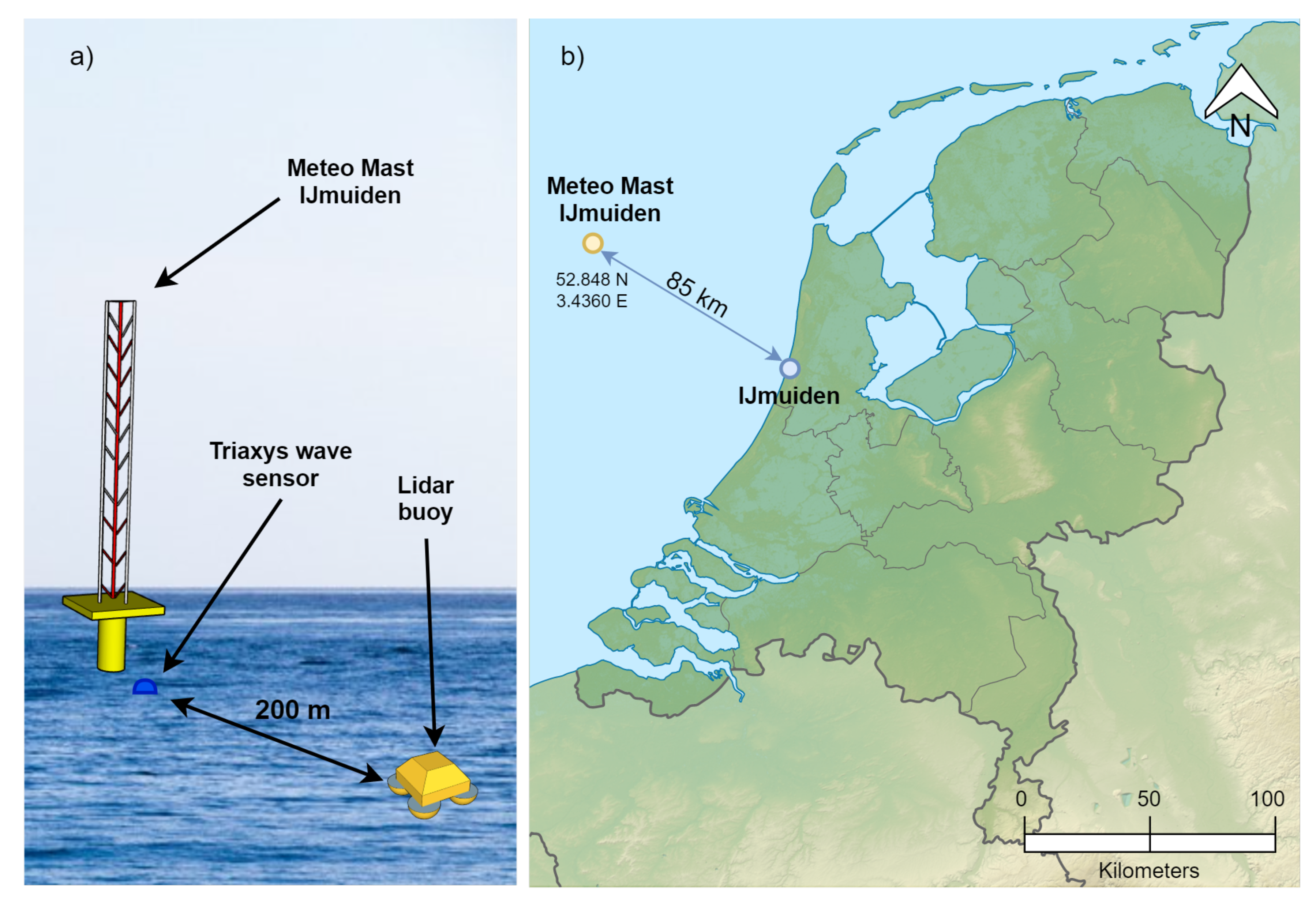
Abstract
1. Introduction
2. Materials and Methods
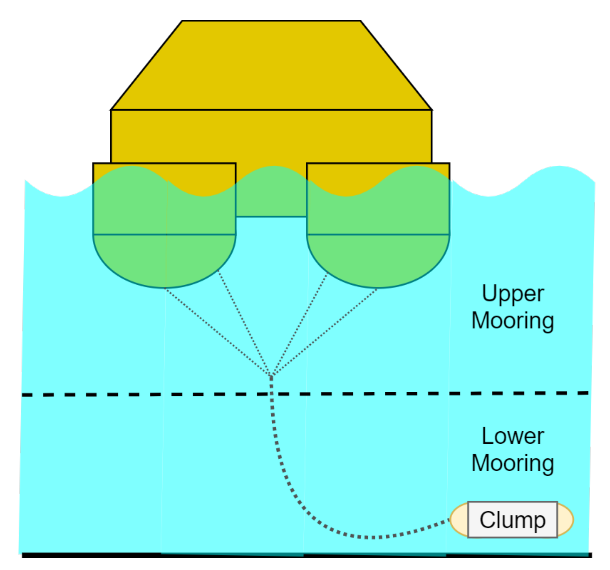
2.1. Materials
2.2. Method (I): Estimation of Sea-Wave Period
- mean zero-crossing period, which is defined as
- average period
- and peak periodwhere is the peak frequency of .
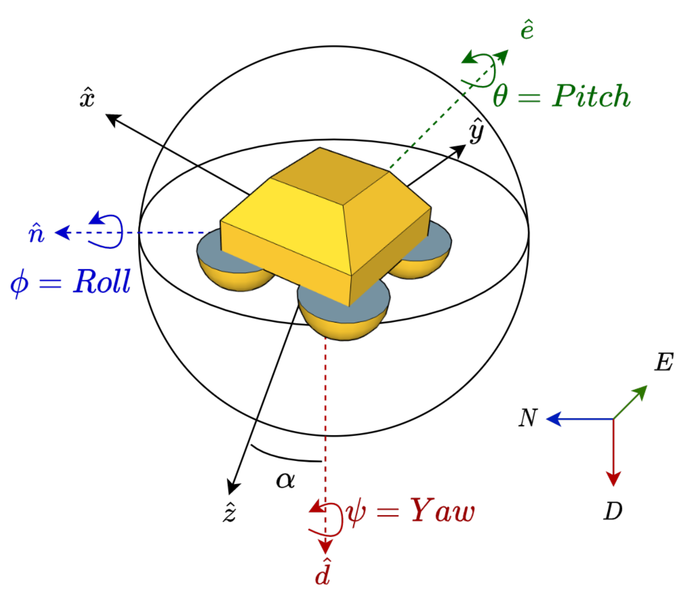
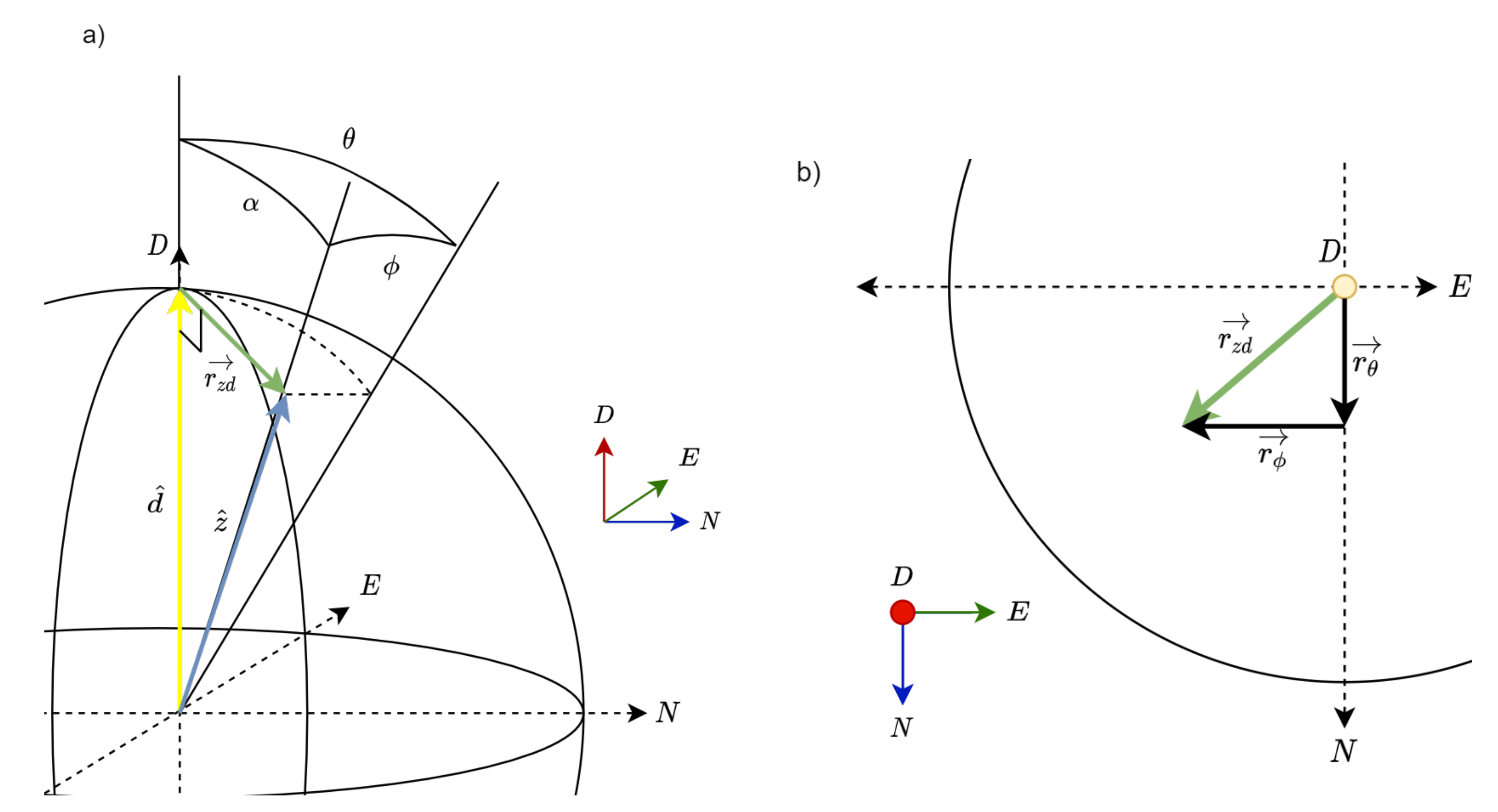
2.3. Method (II): Buoy-Motion Model
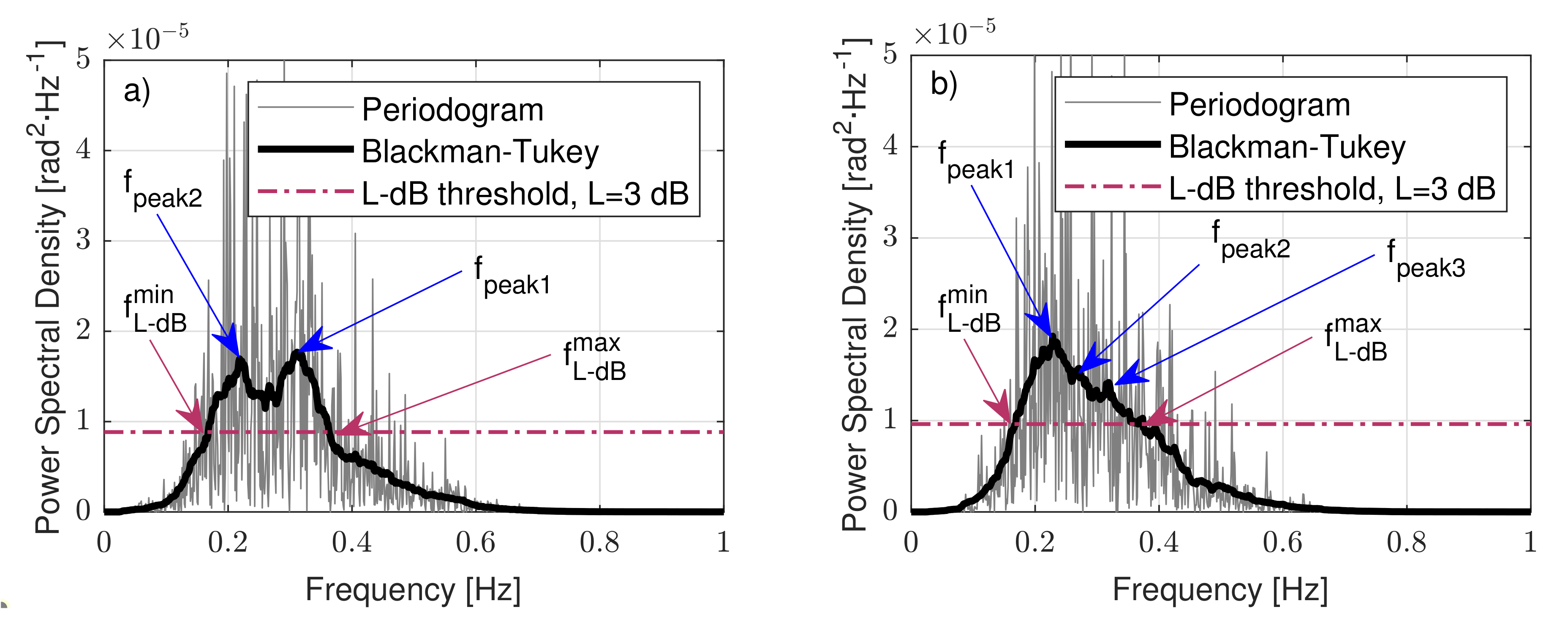
2.4. PSD Estimation
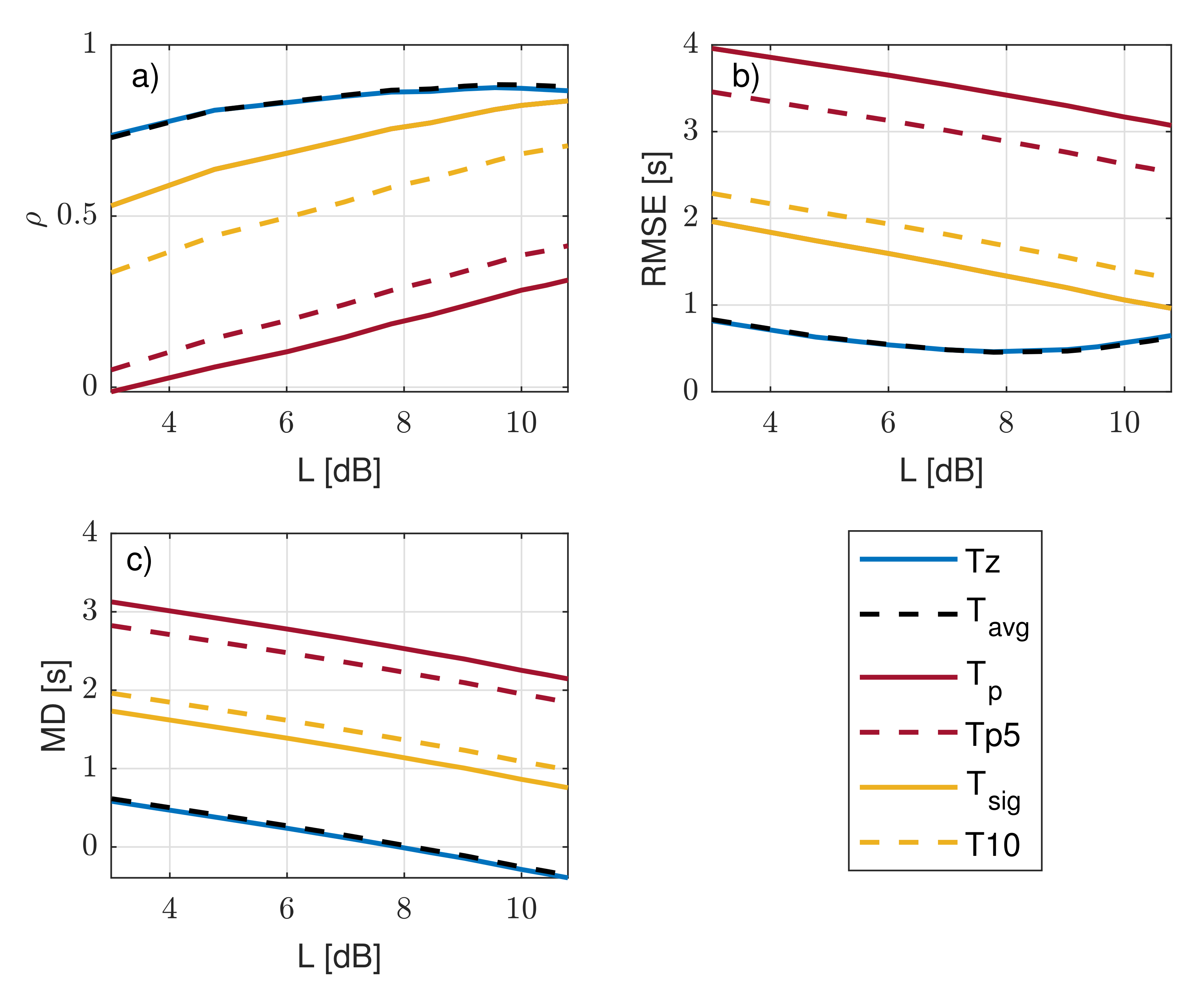
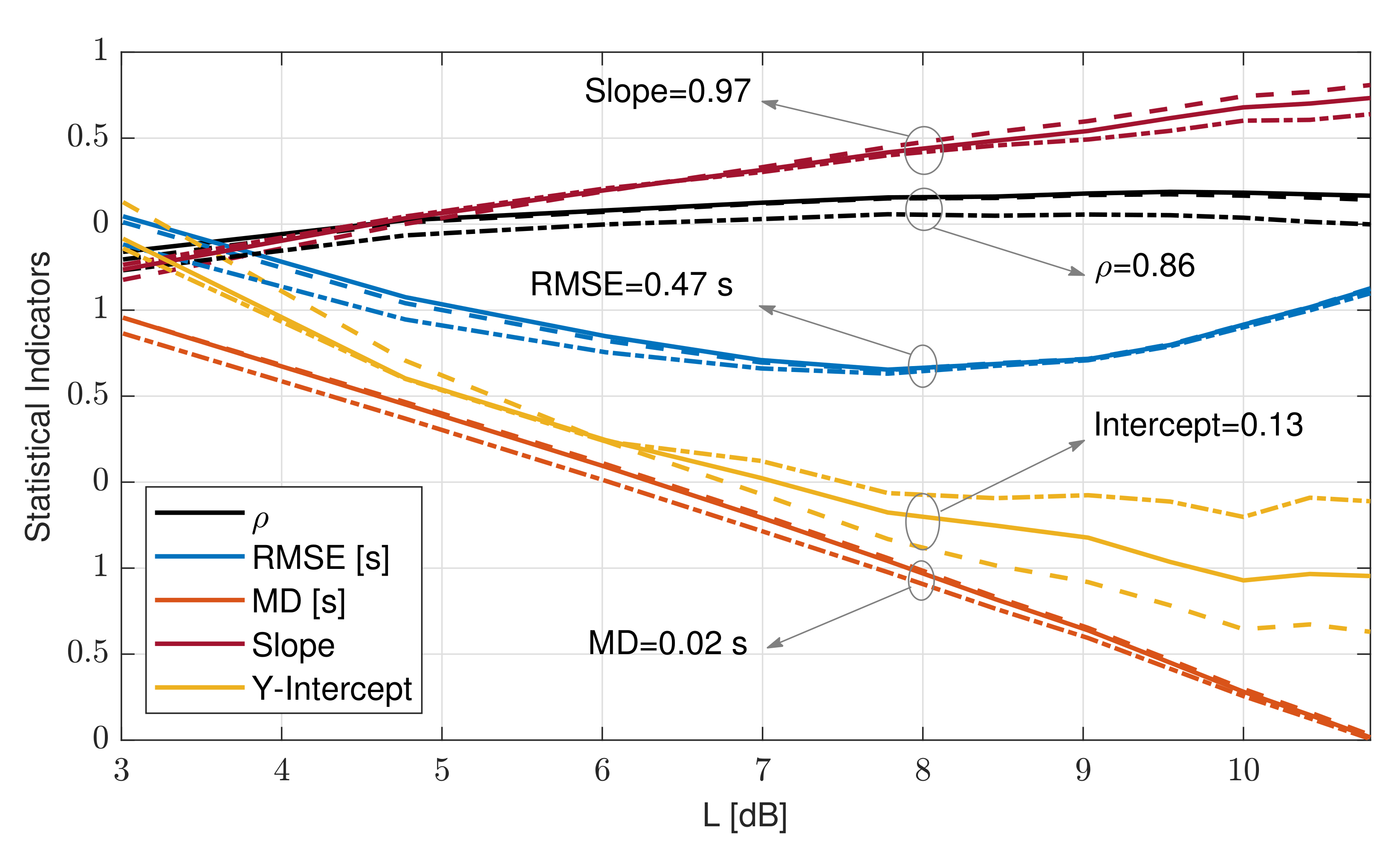
2.5. PSD Significant-Wave-Period Estimation
3. Results and Discussion
4. Summary and Conclusions
Author Contributions
Funding
Institutional Review Board Statement
Informed Consent Statement
Data Availability Statement
Acknowledgments
Conflicts of Interest
Abbreviations
| DOAJ | Directory of open access journals |
| DoF | Degree of freedom |
| DWL | Doppler wind lidar |
| FEM | Fourier expansion method |
| HWS | Horizontal Wind Speed |
| LR | Linear regression |
| MD | Mean deviation |
| MEM | Maximum entropy method |
| NED | North–east–down |
| FFT | Fast Fourier transform |
| IMU | Inertial measurement unit |
| MDPI | Multidisciplinary Digital Publishing Institute |
| Metmast | Meteorological mast |
| PSD | Power spectral density |
| RMSE | Root-mean-square error |
| WE | Wind Energy |
Appendix A. Power-Spectral-Density Derivation
- (i)
- the cross-PSD (also called cross spectral density) between two processes and is the Fourier transform () of the cross-correlation function, , and
- (ii)
- according to the conjugation property, , with X the of signal and the arrow symbol denoting ,
References
- Global Wind Energy Council. Global Wind Report 2018; Technical Report; Global Wind Energy Council: Brussels, Belgium, 2019. [Google Scholar]
- Offshore Wind in Europe Key Trends and Statistics 2019; Technical Report; WindEurope: Brussels, Belgium, 2020.
- Timmons, D. 25—Optimal Renewable Energy Systems: Minimizing the Cost of Intermittent Sources and Energy Storage. In A Comprehensive Guide to Solar Energy Systems; Letcher, T.M., Fthenakis, V.M., Eds.; Academic Press: Cambridge, MA, USA, 2018; pp. 485–504. [Google Scholar] [CrossRef]
- Carbon Trust. Carbon Trust Offshore Wind Accelerator Roadmap for the Commercial Acceptance of Floating LIDAR Technology; Technical Report; Carbon Trust: London, UK, 2013. [Google Scholar]
- Courtney, M.S.; Hasager, C.B. Remote Sensing Technologies for Measuring Offshore Wind. In Offshore Wind Farms; Elsevier: Amsterdam, The Netherlands, 2016; Chapter 4; pp. 59–82. [Google Scholar]
- Antoniou, I.; Jorgensen, H.E.; Mikkelsen, T.; Frandsen, S.; Barthelmie, R.; Perstrup, C.; Hurtig, M. Offshore wind profile measurements from remote sensing instruments. In Proceedings of the European Wind Energy Association Conference & Exhibition 2006, Athens, Greece, 27 February–2 March 2006; European Wind Energy Association Conference & Exhibition: Athens, Greece, 2006; Volume 1, pp. 471–480. [Google Scholar]
- Pichugina, Y.; Banta, R.; Brewer, W.; Sandberg, S.; Hardesty, R. Doppler Lidar–Based Wind-Profile Measurement System for Offshore Wind-Energy and Other Marine Boundary Layer Applications. J. Appl. Meteorol. Climatol. 2012, 51, 327–349. [Google Scholar] [CrossRef]
- Gottschall, J.; Wolken-Möhlmann, G.; Lange, B. About offshore resource assessment with floating lidars with special respect to turbulence and extreme events. J. Phys. Conf. Ser. 2014, 555, 12–43. [Google Scholar] [CrossRef]
- Tiana-Alsina, J.; Rocadenbosch, F.; Gutierrez-Antunano, M.A. Vertical Azimuth Display simulator for wind-Doppler lidar error assessment. In Proceedings of the 2017 IEEE International Geoscience and Remote Sensing Symposium (IGARSS), Fort Worth, TX, USA, 23–28 July 2017; pp. 1614–1617. [Google Scholar] [CrossRef]
- Kelberlau, F.; Neshaug, V.; Lønseth, L.; Bracchi, T.; Mann, J. Taking the Motion out of Floating Lidar: Turbulence Intensity Estimates with a Continuous-Wave Wind Lidar. Remote Sens. 2020, 12, 898. [Google Scholar] [CrossRef]
- Gutiérrez-Antuñano, M.; Tiana-Alsina, J.; Salcedo, A.; Rocadenbosch, F. Estimation of the Motion-Induced Horizontal-Wind-Speed Standard Deviation in an Offshore Doppler Lidar. Remote Sens. 2018, 10, 2037. [Google Scholar] [CrossRef]
- Mangat, M.; des Roziers, E.B.; Medley, J.; Pitter, M.; Barker, W.; Harris, M. The impact of tilt and inflow angle on ground based lidar wind measurements. In Proceedings of the EWEA 2014 Proceedings, The European Wind Energy Associationm, Barcelona, Spain, 10–13 March 2014. [Google Scholar]
- Pitter, E.B.d.R.M.; Medley, J.; Mangat, M.; Slinger, C.; Harris, M. Performance Stability of Zephir in High Motion Enviroments: Floating and Turbine Mounted; Technical Report; ZephIR: Ledbury, UK, 2014. [Google Scholar]
- Bischoff, O.; Würth, I.; Cheng, P.; Tiana-Alsina, J.; Gutiérrez, M. Motion effects on lidar wind measurement data of the EOLOS buoy. In Proceedings of the Renewable Energies Offshore—1st International Conference on Renewable Energies Offshore, RENEW 2014, Lisbon, Portugal, 24–26 November 2014; pp. 197–203. [Google Scholar]
- Gottschall, J.; Lilov, H.; Wolken-Möhlmann, G.; Lange, B. Lidars on floating offshore platforms; About the correction of motion-induced lidar measurement errors. In Proceedings of the EWEA 2012 Proceedings, The European Wind Energy Association, Lisbon, Portugal, 16–19 April 2012. [Google Scholar]
- Schuon, F.; González, D.; Rocadenbosch, F.; Bischoff, O.; Jané, R. KIC InnoEnergy Project Neptune: Development of a Floating LiDAR Buoy for Wind, Wave and Current Measurements. In Proceedings of the DEWEK 2012 German Wind Energy Conference, Bremen, Germany, 19–20 May 2012. [Google Scholar]
- N.D.B. Center. Nondirectional and Directional Wave Data Analysis Procedures; Technical Report; National Oceanic and Atmospheric Administration: Washington, DC, USA, 1996. [Google Scholar]
- Faltinsen, O. Sea Loads on Ships and Offshore Structures; Cambridge University Press: Cambridge, UK, 1993; Volume 1. [Google Scholar]
- Suh, K.D.; Kwon, H.D.; Lee, D.Y. Some statistical characteristics of large deepwater waves around the Korean Peninsula. Coast. Eng. 2010, 57, 375–384. [Google Scholar] [CrossRef]
- Ardhuin, F.; Stopa, J.E.; Chapron, B.; Collard, F.; Husson, R.; Jensen, R.E.; Johannessen, J.; Mouche, A.; Passaro, M.; Quartly, G.D.; et al. Observing Sea States. Front. Mar. Sci. 2019, 6, 124. [Google Scholar] [CrossRef]
- Chun, H.; Suh, K.-D. Estimation of significant wave period from wave spectrum. J. Ocean. Eng. Technol. 2018, 163, 609–616. [Google Scholar] [CrossRef]
- Gottschall, J.; Catalano, E.; Dörenkämper, M.; Witha, B. The NEWA Ferry Lidar Experiment: Measuring Mesoscale Winds in the Southern Baltic Sea. Remote Sens. 2018, 10, 1620. [Google Scholar] [CrossRef]
- He, Y.; Fu, J.; Shu, Z.; Chan, P.; Wu, J.; Li, Q. A comparison of micrometeorological methods for marine roughness estimation at a coastal area. J. Wind. Eng. Ind. Aerodyn. 2019, 195, 104010. [Google Scholar] [CrossRef]
- Kuik, A.J.; van Vledder, G.P.; Holthuijsen, L.H. A Method for the Routine Analysis of Pitch-and-Roll Buoy Wave Data. J. Phys. Oceanogr. 1988, 18, 1020–1034. [Google Scholar] [CrossRef]
- Gutiérrez-Antuñano, M.A.; Tiana-Alsina, J.; Rocadenbosch, F. Performance evaluation of a floating lidar buoy in nearshore conditions. Wind Energy 2017, 20, 1711–1726. [Google Scholar] [CrossRef]
- Salcedo-Bosch, A.; Gutierrez-Antunano, M.A.; Tiana-Alsina, J.; Rocadenbosch, F. Motional Behavior Estimation Using Simple Spectral Estimation: Application to the Off-Shore Wind Lidar. In Proceedings of the 2020 IEEE International Geoscience and Remote Sensing Symposium, (IGARSS-2020), Virtual Event, 26 September–2 October 2020; Available online: https://igarss2020.org/ (accessed on 27 September 2020).
- Gutierrez-Antunano, M.A.; Tiana-Alsina, J.; Rocadenbosch, F.; Sospedra, J.; Aghabi, R.; Gonzalez-Marco, D. A wind-lidar buoy for offshore wind measurements: First commissioning test-phase results. In Proceedings of the 2017 IEEE International Geoscience and Remote Sensing Symposium (IGARSS-2017), Fort Worth, TX, USA, 23–28 July 2017; pp. 1607–1610. [Google Scholar] [CrossRef]
- Sospedra, J.; Cateura, J.; Puigdefàbregas, J. Novel multipurpose buoy for offshore wind profile measurements EOLOS platform faces validation at ijmuiden offshore metmast. Sea Technol. 2015, 56, 25–28. [Google Scholar]
- Werkhoven, E.J.; Verhoef, J.P. Offshore Meteorological Mast Ijmuiden Abstract of Instrumentation Report; Technical Report; Energy Research Centre of the Netherlands (ECN): Petten, The Netherlands, 2012. [Google Scholar]
- NordNordWest. Netherlands Relief Location Map. 2008. Available online: https://creativecommons.org/licenses/by-sa/3.0/de/legalcode (accessed on 3 November 2020).
- Gutiérrez Antuñano, M.Á. Doppler Wind LIDAR Systems Data Processing and Applications: An Overview Towards Developing the New Generation of Wind Remote-Sensing Sensors for Off-Shore Wind Farms. Ph.D. Thesis, UPC, Departament de Teoria del Senyal i Comunicacions, Barcelona, Spain, 2019. [Google Scholar]
- AXYS Technologies. TRIAXIS Sensor; AXYS Technologies: Sidney, BC, Canada, 2015. [Google Scholar]
- MacIsaac, C.; Naeth, S. TRIAXYS Next Wave II Directional Wave Sensor The evolution of wave measurements. In Proceedings of the 2013 OCEANS, San Diego, CA, USA, 23–27 September 2013; pp. 1–8. [Google Scholar]
- Auestad, Ø.F.; Gravdahl, J.T.; Fossen, T.I. Heave Motion Estimation on a Craft Using a Strapdown Inertial Measurement Unit. In Proceedings of the 9th IFAC Conference on Control Applications in Marine Systems, IFAC, Osaka, Japan, 17–20 September 2013; Volume 46, pp. 298–303. [Google Scholar] [CrossRef]
- Barstow, S.F.; Bidlot, J.R.; Caires, S.; Donelan, M.; Drennan, W.E.A. Measuring and Analysing the Directional Spectra of Ocean Waves; Number EUR 21367; COST Office: Brussels, Belgium, 2005. [Google Scholar]
- Tannuri, E.; Sparano, J.; Simos, A.; Cruz, J.D. Estimating directional wave spectrum based on stationary ship motion measurements. Appl. Ocean Res. 2003, 25, 243–261. [Google Scholar] [CrossRef]
- Massel, S.R. Ocean Surface Waves: Their Physics and Prediction; World Scientific Publishing Company: Singapore, 2017; Volume 45. [Google Scholar]
- Sweitzer, K.A.; Bishop, N.W.; Genberg, V.L. Efficient computation of spectral moments for determination of random response statistics. In Proceedings of the ISMA, Leuven, Belgium, 20–22 September 2004; pp. 2677–2692. [Google Scholar]
- Roithmayr, C.M.; Hodges, D.H. Dynamics: Theory and Application of Kane’s Method. J. Comput. Nonlinear Dyn. 2016, 11, 6. [Google Scholar] [CrossRef]
- Proakis, J.; Manolakis, D. Digital Signal Processing, 4th ed.; Prentice Hall: Upper Saddle River, NJ, USA, 2006. [Google Scholar]
- Brillouin, L.; Massey, H. Wave Propagation and Group Velocity, Pure and Applied Physics; Elsevier Science: Amsterdam, The Netherlands, 2013; Volume 8. [Google Scholar]
- Ricci, A.; Blocken, B. On the reliability of the 3D steady RANS approach in predicting microscale wind conditions in seaport areas: The case of the IJmuiden sea lock. J. Wind. Eng. Ind. Aerodyn. 2020, 207, 104437. [Google Scholar] [CrossRef]
- Bracewell, R. The Fourier Transform and Its Applications; Circuits and Systems; McGraw Hill: New York, NY, USA, 2000. [Google Scholar]


Publisher’s Note: MDPI stays neutral with regard to jurisdictional claims in published maps and institutional affiliations. |
© 2021 by the authors. Licensee MDPI, Basel, Switzerland. This article is an open access article distributed under the terms and conditions of the Creative Commons Attribution (CC BY) license (http://creativecommons.org/licenses/by/4.0/).
Share and Cite
Salcedo-Bosch, A.; Rocadenbosch, F.; Gutiérrez-Antuñano, M.A.; Tiana-Alsina, J. Estimation of Wave Period from Pitch and Roll of a Lidar Buoy. Sensors 2021, 21, 1310. https://doi.org/10.3390/s21041310
Salcedo-Bosch A, Rocadenbosch F, Gutiérrez-Antuñano MA, Tiana-Alsina J. Estimation of Wave Period from Pitch and Roll of a Lidar Buoy. Sensors. 2021; 21(4):1310. https://doi.org/10.3390/s21041310
Chicago/Turabian StyleSalcedo-Bosch, Andreu, Francesc Rocadenbosch, Miguel A. Gutiérrez-Antuñano, and Jordi Tiana-Alsina. 2021. "Estimation of Wave Period from Pitch and Roll of a Lidar Buoy" Sensors 21, no. 4: 1310. https://doi.org/10.3390/s21041310
APA StyleSalcedo-Bosch, A., Rocadenbosch, F., Gutiérrez-Antuñano, M. A., & Tiana-Alsina, J. (2021). Estimation of Wave Period from Pitch and Roll of a Lidar Buoy. Sensors, 21(4), 1310. https://doi.org/10.3390/s21041310