
Optical Flow Estimation by Matching Time Surface with Event-Based Cameras


Abstract
1. Introduction
- We propose the loss function measuring the timestamp consistency of the time surface for optical flow estimation using event-based cameras. This proposed loss function makes it possible to estimate dense optical flows without explicitly reconstructing image intensity or utilizing additional sensor information.
- Visualizing the loss landscape, we show that our loss is more stable regardless of the texture than the variance used in the motion compensation framework. Alongside this, we also show that the gradient is calculated in the correct direction in our method even around a line segment.
- We evaluate the dense optical flow estimated by optimization with L1 smoothness regularization. Our method recodes with higher accuracy compared with the conventional methods in the various scenes from the two publicly available datasets.
2. Related Work
3. Methodology
3.1. Event Representation
3.2. Time Surface
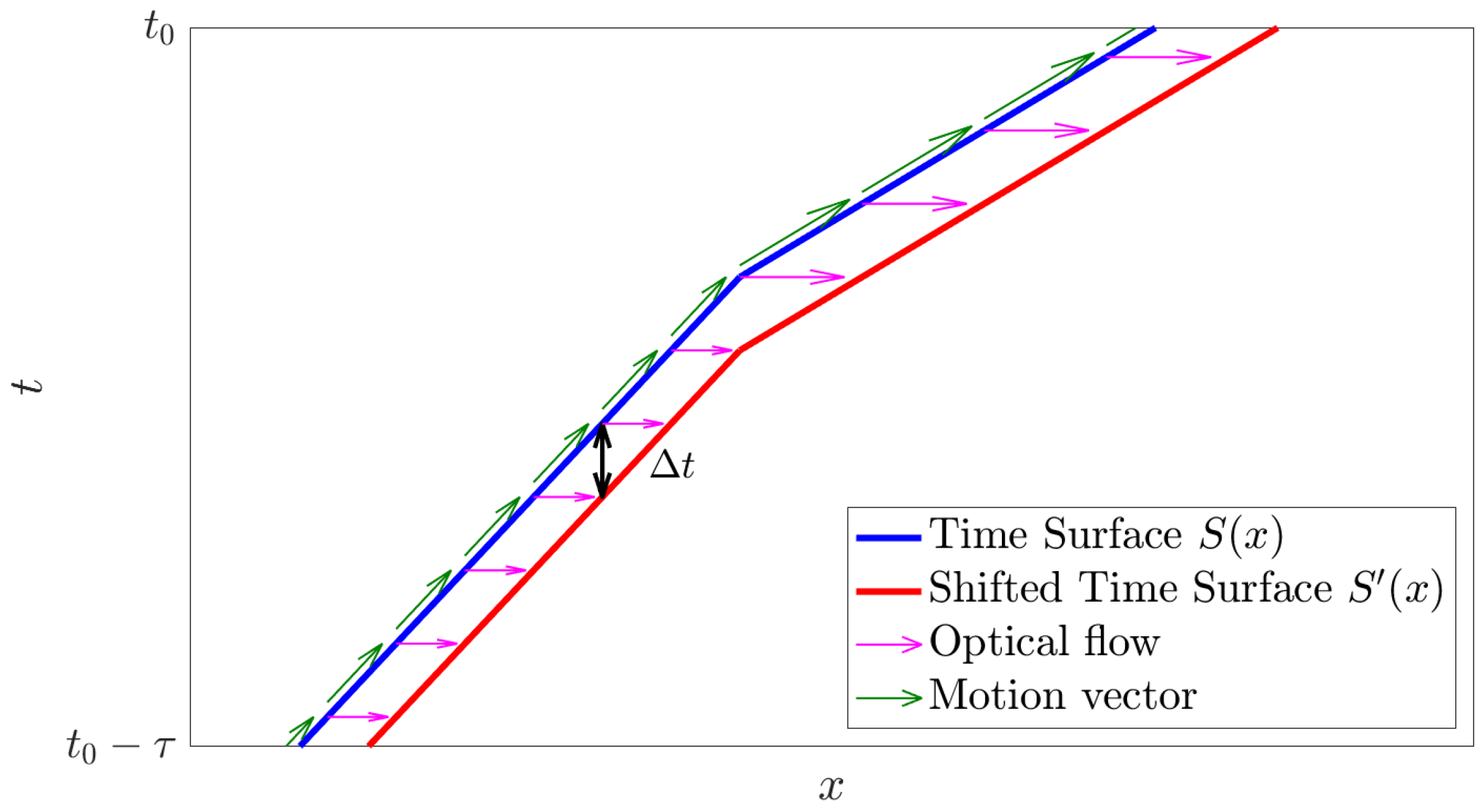
3.3. Surface Matching Loss
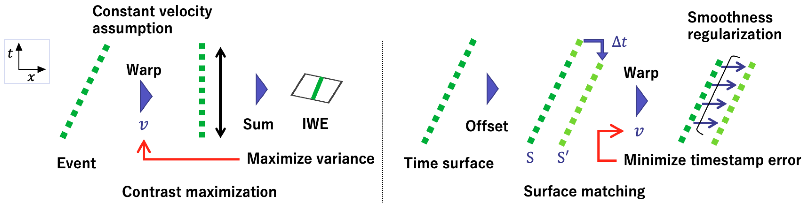
3.4. Comparison with Contrast Maximization
4. Experiment
4.1. Datasets
- ESIM
- An Open Event Camera Simulator (ESIM) [28] can accurately and efficiently simulate an event-based camera and output a set of events and the ground truth of optical flows with any camera motion and scene.
- MVSEC
- The Multi-Vehicle Stereo Event Camera Dataset (MVSEC) [29] contains an outdoor driving scene—by day and by night—and an indoor flight scene by the drone. The event-based camera used is mDAVIS-346B with a resolution of 346 × 260, which can capture general images simultaneously. The dataset provides the ground truth optical flow generated from depth maps by LiDAR and poses information by the Inertial Measurement Unit (IMU).
- HACD
- The HVGA ATIS Corner Dataset (HACD) [25] is built with a recording of planar patterns to evaluate corner detectors. Those sequences were taken by an Asynchronous Time-based Image Sensor (ATIS) [30] with a resolution of 480 × 360. It also contains the position of markers at four corners of the poster, each 10 ms. With this information, the homography of the plane can be calculated, and the ground truth optical flow at any point on the poster can be obtained.
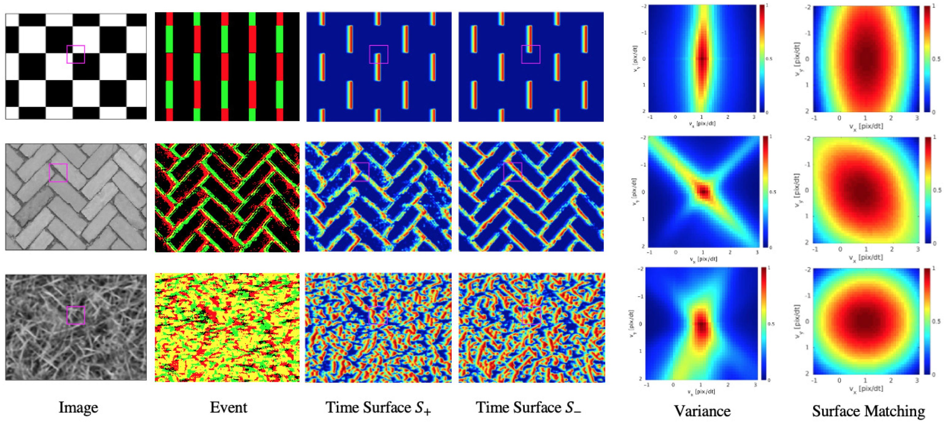
4.2. Loss Landscape
- Variance The variance loss represented by Equation (11). Events are warped by the optical flow which is common at all pixels. The duration of the events used and the time interval of the optical flow were set to and in order to match our method with the condition.
- Surface Matching Loss The proposed loss function represented by Equation (7). This loss is calculated by the difference between the time surface and the shifted time surface warped by the optical flow. The sign has been inverted to match the variance.
- Results and discussions
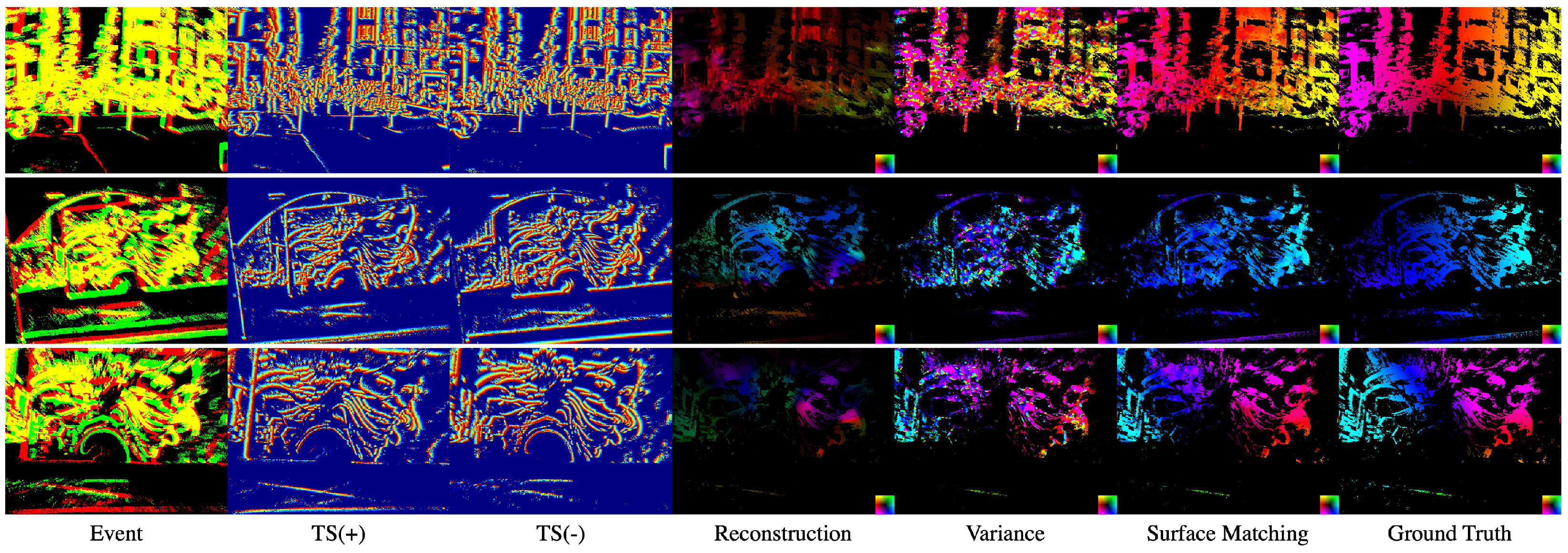
4.3. Dense Optical Flow Estimation
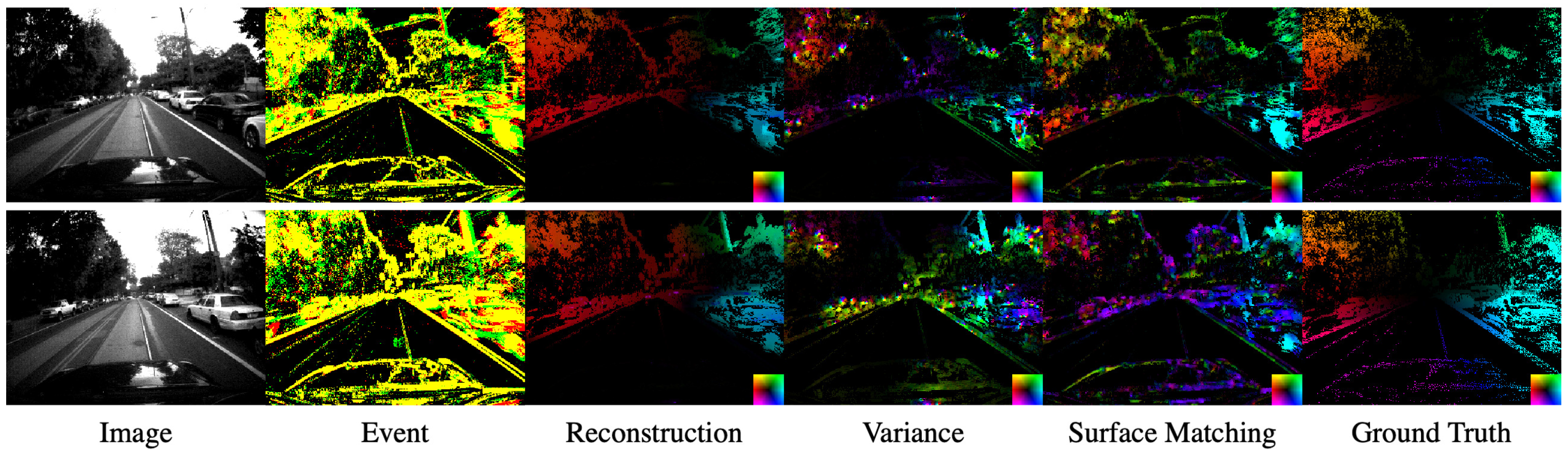
- Reconstruction The method for estimating optical flow simultaneously with luminance restoration [9]. A large number of optical flows and image parameters were optimized under a temporal smoothness assumption sequentially in the sliding window containing the events with a duration of 128 .
- Variance The method of maximizing a variance of the IWE [10]. In [10], the optical flow parameters were common in the patches, but in order to make the conditions uniform, a dense optical flow estimation was performed by adding the L1 smoothness regularization as follows:Events were warped by the optical flow at each pixel: . The loss function is optimized by the primal-dual algorithm in the same way as the TV-L1 method [31]. The duration of the events used was set to to match our method.
- Surface Matching Our proposed method rewritten as follows:
- Qualitative result
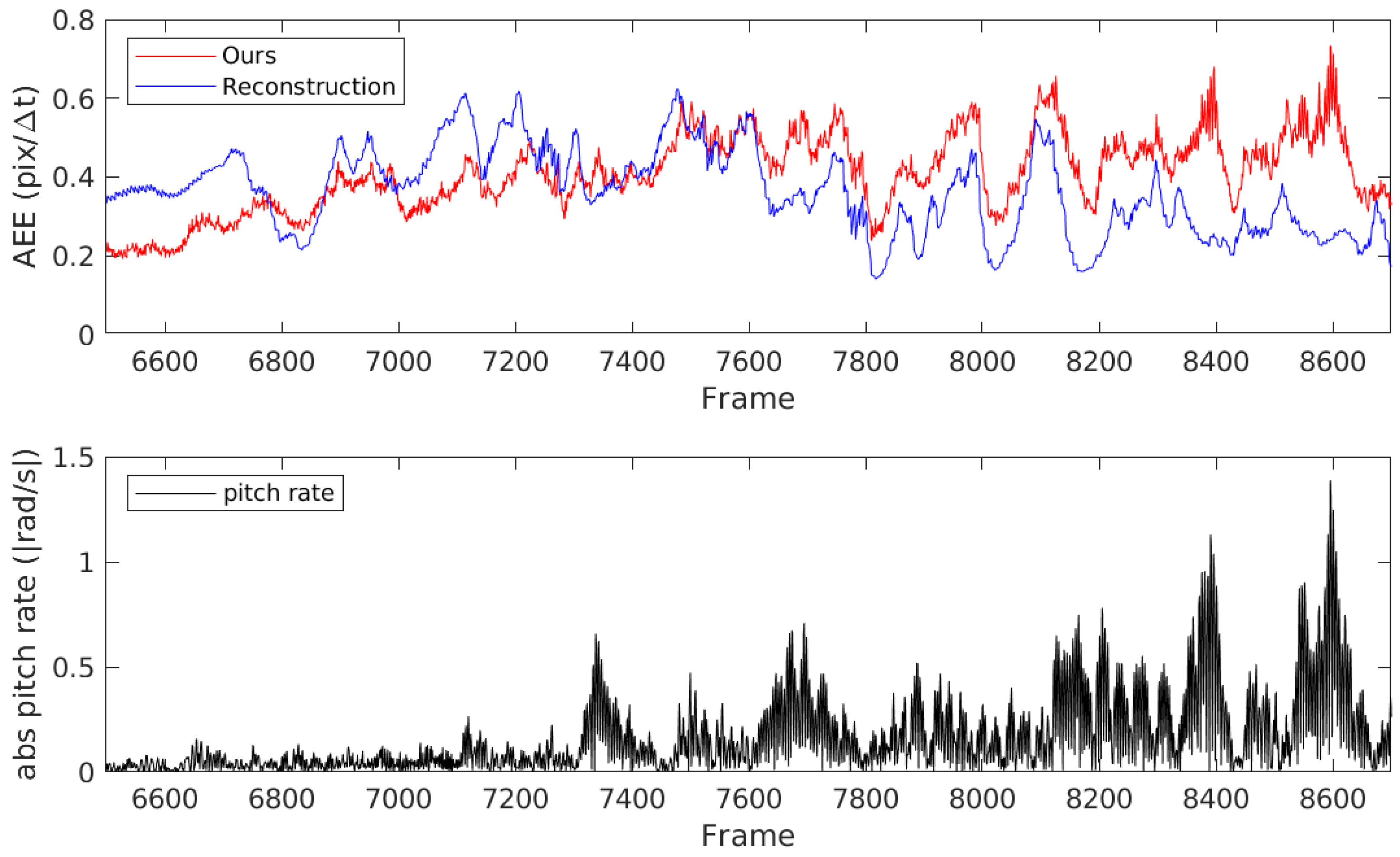
- Quantitative result
4.4. Study on Hyperparameters
5. Conclusions
Author Contributions
Funding
Institutional Review Board Statement
Informed Consent Statement
Data Availability Statement
Conflicts of Interest
References
- Gallego, G.; Delbruck, T.; Orchard, G.; Bartolozzi, C.; Taba, B.; Censi, A.; Leutenegger, S.; Davison, A.; Conradt, J.; Daniilidis, K.; et al. Event-based Vision: A Survey. arXiv 2019, arXiv:1904.08405. [Google Scholar]
- Kim, H.; Handa, A.; Benosman, R.; Ieng, S.H.; Davison, A. Simultaneous Mosaicing and Tracking with an Event Camera. In Proceedings of the British Machine Vision Conference (BMVC), Nottingham, UK, 1–5 September 2014. [Google Scholar] [CrossRef]
- Kim, H.; Leutenegger, S.; Davison, A.J. Real-time 3D reconstruction and 6-DoF tracking with an event camera. In Proceedings of the European Conference on Computer Vision (ECCV), Amsterdam, The Netherlands, 11–14 October 2016; pp. 349–364. [Google Scholar] [CrossRef]
- Rebecq, H.; Ranftl, R.; Koltun, V.; Scaramuzza, D. Events-to-Video: Bringing Modern Computer Vision to Event Cameras. In Proceedings of the IEEE Conference on Computer Vision and Pattern Recognition (CVPR), Long Beach, CA, USA, 16–20 June 2019; pp. 3857–3866. [Google Scholar]
- Lucas, B.D.; Kanade, T. An Iterative Image Registration Technique with an Application to Stereo Vision. 1981. Available online: https://ri.cmu.edu/pub_files/pub3/lucas_bruce_d_1981_2/lucas_bruce_d_1981_2.pdf (accessed on 20 January 2021).
- Horn, B.K.B.; Schunck, B.G. Determining Optical Flow. Artif. Intell. 1981, 17, 185–203. [Google Scholar] [CrossRef]
- Benosman, R.; Ieng, S.H.; Clercq, C.; Bartolozzi, C.; Srinivasan, M. Asynchronous frameless event-based optical flow. Neural Netw. 2012, 27, 32–37. [Google Scholar] [CrossRef] [PubMed]
- Brosch, T.; Tschechne, S.; Neumann, H. On event-based optical flow detection. Front. Neurosci. 2015. [Google Scholar] [CrossRef] [PubMed]
- Bardow, P.; Davison, A.J.; Leutenegger, S. Simultaneous Optical Flow and Intensity Estimation from an Event Camera. In Proceedings of the IEEE Conference on Computer Vision and Pattern Recognition (CVPR), Las Vegas, NV, USA, 27–30 June 2016; pp. 884–892. [Google Scholar] [CrossRef]
- Gallego, G.; Rebecq, H.; Scaramuzza, D. A Unifying Contrast Maximization Framework for Event Cameras, with Applications to Motion, Depth, and Optical Flow Estimation. In Proceedings of the IEEE Conference on Computer Vision and Pattern Recognition (CVPR), Salt Lake City, UT, USA, 18–22 June 2018; pp. 3867–3876. [Google Scholar] [CrossRef]
- Zhu, A.Z.; Yuan, L.; Chaney, K.; Daniilidis, K. Unsupervised Event-based Learning of Optical Flow, Depth, and Egomotion. In Proceedings of the IEEE Conference on Computer Vision and Pattern Recognition (CVPR), Long Beach, CA, USA, 16–20 June 2019; pp. 989–997. [Google Scholar]
- Gallego, G.; Gehrig, M.; Scaramuzza, D. Focus Is All You Need: Loss Functions for Event-Based Vision. In Proceedings of the IEEE Conference on Computer Vision and Pattern Recognition (CVPR), Long Beach, CA, USA, 16–20 June 2019; pp. 12272–12281. [Google Scholar] [CrossRef]
- Mueggler, E.; Rebecq, H.; Gallego, G.; Delbruck, T.; Scaramuzza, D. The Event-Camera Dataset and Simulator: Event-based Data for Pose Estimation, Visual Odometry, and SLAM. Int. J. Robot. Res. 2017, 36, 142–149. [Google Scholar] [CrossRef]
- Brandli, C.; Berner, R.; Yang, M.; Liu, S.C.; Delbruck, T. A 240 × 180 130 dB 3 μs latency global shutter spatiotemporal vision sensor. IEEE J. Solid State Circuits 2014, 49, 2333–2341. [Google Scholar] [CrossRef]
- Benosman, R.; Clercq, C.; Lagorce, X.; Sio-Hoi, I.; Bartolozzi, C. Event-Based Visual Flow. IEEE Trans. Neural Netw. Learn. Syst. 2014, 25, 407–417. [Google Scholar] [CrossRef] [PubMed]
- Rueckauer, B.; Delbruck, T. Evaluation of Event-Based Algorithms for Optical Flow with Ground-Truth from Inertial Measurement Sensor. Front. Neurosci. 2016, 10. [Google Scholar] [CrossRef] [PubMed]
- Zhu, A.; Yuan, L.; Chaney, K.; Daniilidis, K. EV-FlowNet: Self-Supervised Optical Flow Estimation for Event-based Cameras. Robot. Sci. Syst. 2018. [Google Scholar] [CrossRef]
- Ye, C.; Mitrokhin, A.; Fermüller, C.; Yorke, J.A.; Aloimonos, Y. Unsupervised Learning of Dense Optical Flow, Depth and Egomotion from Sparse Event Data. arXiv 2018, arXiv:1809.08625. [Google Scholar]
- Gallego, G.; Scaramuzza, D. Accurate Angular Velocity Estimation With an Event Camera. IEEE Robot. Autom. Lett. 2017, 2, 632–639. [Google Scholar] [CrossRef]
- Zhu, A.Z.; Atanasov, N.; Daniilidis, K. Event-based feature tracking with probabilistic data association. In Proceedings of the IEEE International Conference on Robotics and Automation (ICRA), Singapore, 29 May–3 June 2017; pp. 4465–4470. [Google Scholar] [CrossRef]
- Stoffregen, T.; Kleeman, L. Simultaneous Optical Flow and Segmentation (SOFAS) using Dynamic Vision Sensor. In Proceedings of the Australasian Conference on Robotics and Automation (ACRA), Sydney, Australia, 11–13 December 2017; pp. 52–61. [Google Scholar]
- Mitrokhin, A.; Fermuller, C.; Parameshwara, C.; Aloimonos, Y. Event-Based Moving Object Detection and Tracking. In Proceedings of the IEEE International Conference on Intelligent Robots and Systems (IROS), Madrid, Spain, 1–5 October 2018; pp. 1–9. [Google Scholar] [CrossRef]
- Stoffregen, T.; Kleeman, L. Event Cameras, Contrast Maximization and Reward Functions: An Analysis. In Proceedings of the IEEE/CVF Conference on Computer Vision and Pattern Recognition, Long Beach, CA, USA, 15–20 June 2019. [Google Scholar]
- Lagorce, X.; Orchard, G.; Galluppi, F.; Shi, B.E.; Benosman, R.B. HOTS: A Hierarchy of Event-Based Time-Surfaces for Pattern Recognition. IEEE Trans. Pattern Anal. Mach. Intell. 2017, 39, 1346–1359. [Google Scholar] [CrossRef] [PubMed]
- Manderscheid, J.; Sironi, A.; Bourdis, N.; Migliore, D.; Lepetit, V. Speed Invariant Time Surface for Learning to Detect Corner Points With Event-Based Cameras. In Proceedings of the IEEE Conference on Computer Vision and Pattern Recognition (CVPR), Long Beach, CA, USA, 16–20 June 2019; pp. 10237–10246. [Google Scholar] [CrossRef]
- Zach, C.; Pock, T.; Bischof, H. A Duality Based Approach for Realtime TV-L1 Optical Flow. Pattern Recognit. 2007, 214–223. [Google Scholar] [CrossRef]
- Sánchez Pérez, J.; Meinhardt-Llopis, E.; Facciolo, G. TV-L1 Optical Flow Estimation. Image Process. Line 2013, 3, 137–150. [Google Scholar] [CrossRef]
- Rebecq, H.; Gehrig, D.; Scaramuzza, D. ESIM: An Open Event Camera Simulator. Conf. Robot. Learn. 2018, 87, 969–982. [Google Scholar]
- Zhu, A.Z.; Thakur, D.; Ozaslan, T.; Pfrommer, B.; Kumar, V.; Daniilidis, K. The Multi Vehicle Stereo Event Camera Dataset: An Event Camera Dataset for 3D Perception. IEEE Robot. Autom. Lett. 2018, 3, 2032–2039. [Google Scholar] [CrossRef]
- Posch, C.; Serrano-Gotarredona, T.; Linares-Barranco, B.; Delbruck, T. Retinomorphic event-based vision sensors: Bioinspired cameras with spiking output. Proc. IEEE 2014, 102, 1470–1484. [Google Scholar] [CrossRef]
- Chambolle, A.; Pock, T. A first-order primal-dual algorithm for convex problems with applications to imaging. J. Math. Imaging Vis. 2011, 40, 120–145. [Google Scholar] [CrossRef]


| Day 1 | Day 2 | Night 1 | Night 2 | Night 3 | Flying 1 | Flying 2 | Flying 3 | Guernica | Paris | Graffiti | |
|---|---|---|---|---|---|---|---|---|---|---|---|
| Reconstruction [9] | 0.267 | 0.307 | 0.283 | 0.313 | 0.365 | 0.348 | 0.525 | 0.468 | 1.99 | 2.79 | 1.91 |
| Variance [10] | 0.479 | 0.479 | 0.418 | 0.368 | 0.438 | 0.351 | 0.525 | 0.469 | 4.01 | 3.11 | 1.90 |
| Surface Matching | 0.257 | 0.350 | 0.334 | 0.363 | 0.356 | 0.278 | 0.422 | 0.377 | 1.50 | 2.30 | 1.36 |
| 25 ms | 50 ms | 75 ms | ||
|---|---|---|---|---|
| 2.5 ms | 0.95 | 1.14 | - | |
| 5.0 ms | 1.34 | 1.50 | 1.61 | |
| 7.5 ms | - | 1.74 | 1.81 | |
Publisher’s Note: MDPI stays neutral with regard to jurisdictional claims in published maps and institutional affiliations. |
© 2021 by the authors. Licensee MDPI, Basel, Switzerland. This article is an open access article distributed under the terms and conditions of the Creative Commons Attribution (CC BY) license (http://creativecommons.org/licenses/by/4.0/).
Share and Cite
Nagata, J.; Sekikawa, Y.; Aoki, Y. Optical Flow Estimation by Matching Time Surface with Event-Based Cameras. Sensors 2021, 21, 1150. https://doi.org/10.3390/s21041150
Nagata J, Sekikawa Y, Aoki Y. Optical Flow Estimation by Matching Time Surface with Event-Based Cameras. Sensors. 2021; 21(4):1150. https://doi.org/10.3390/s21041150
Chicago/Turabian StyleNagata, Jun, Yusuke Sekikawa, and Yoshimitsu Aoki. 2021. "Optical Flow Estimation by Matching Time Surface with Event-Based Cameras" Sensors 21, no. 4: 1150. https://doi.org/10.3390/s21041150
APA StyleNagata, J., Sekikawa, Y., & Aoki, Y. (2021). Optical Flow Estimation by Matching Time Surface with Event-Based Cameras. Sensors, 21(4), 1150. https://doi.org/10.3390/s21041150