Comparison of Heating Strategies on Soil Water Measurement Using Actively Heated Fiber Optics on Contrasting Textured Soils

 , and
, and 
Abstract
1. Introduction
2. Materials and Methods
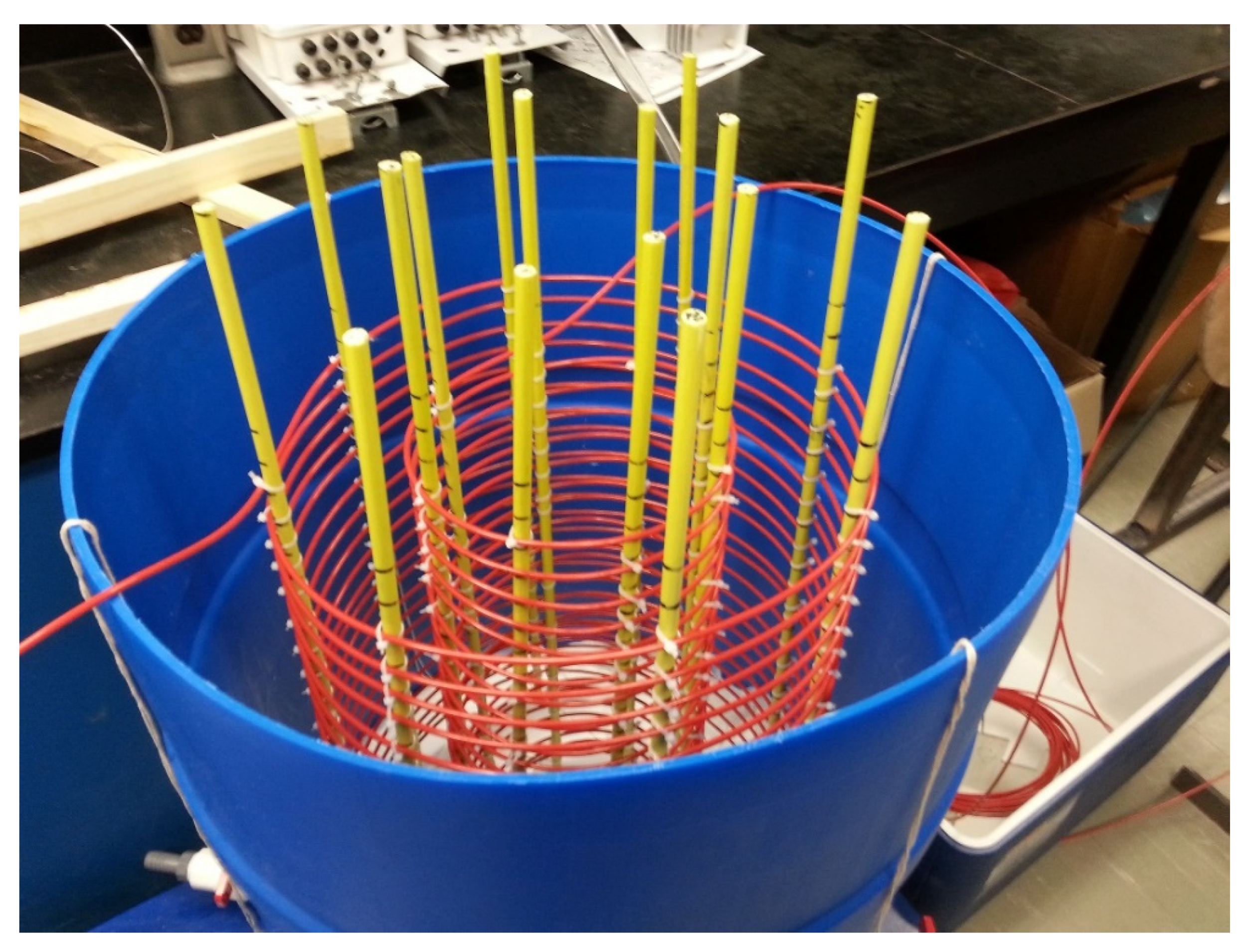
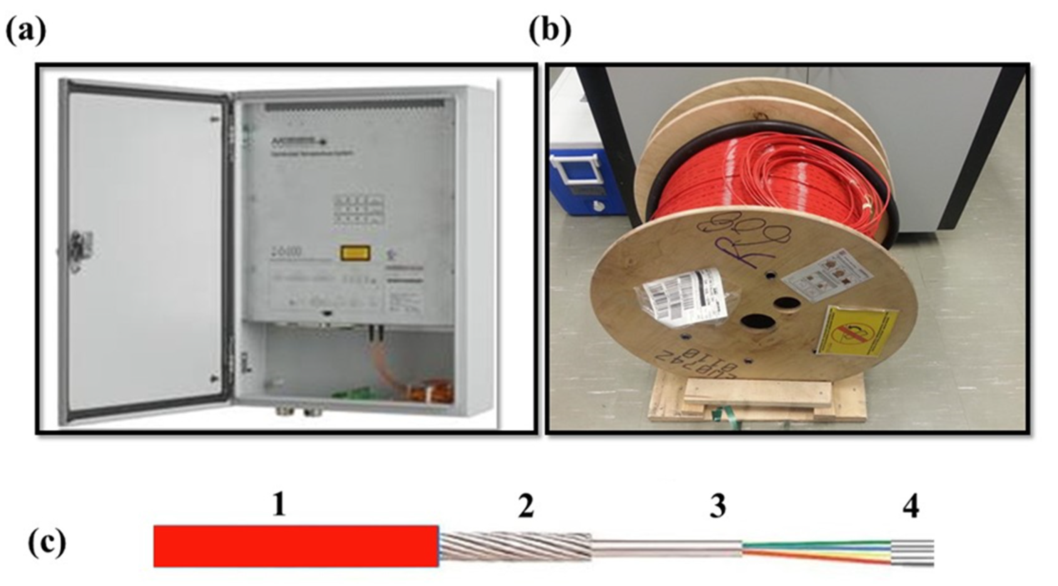
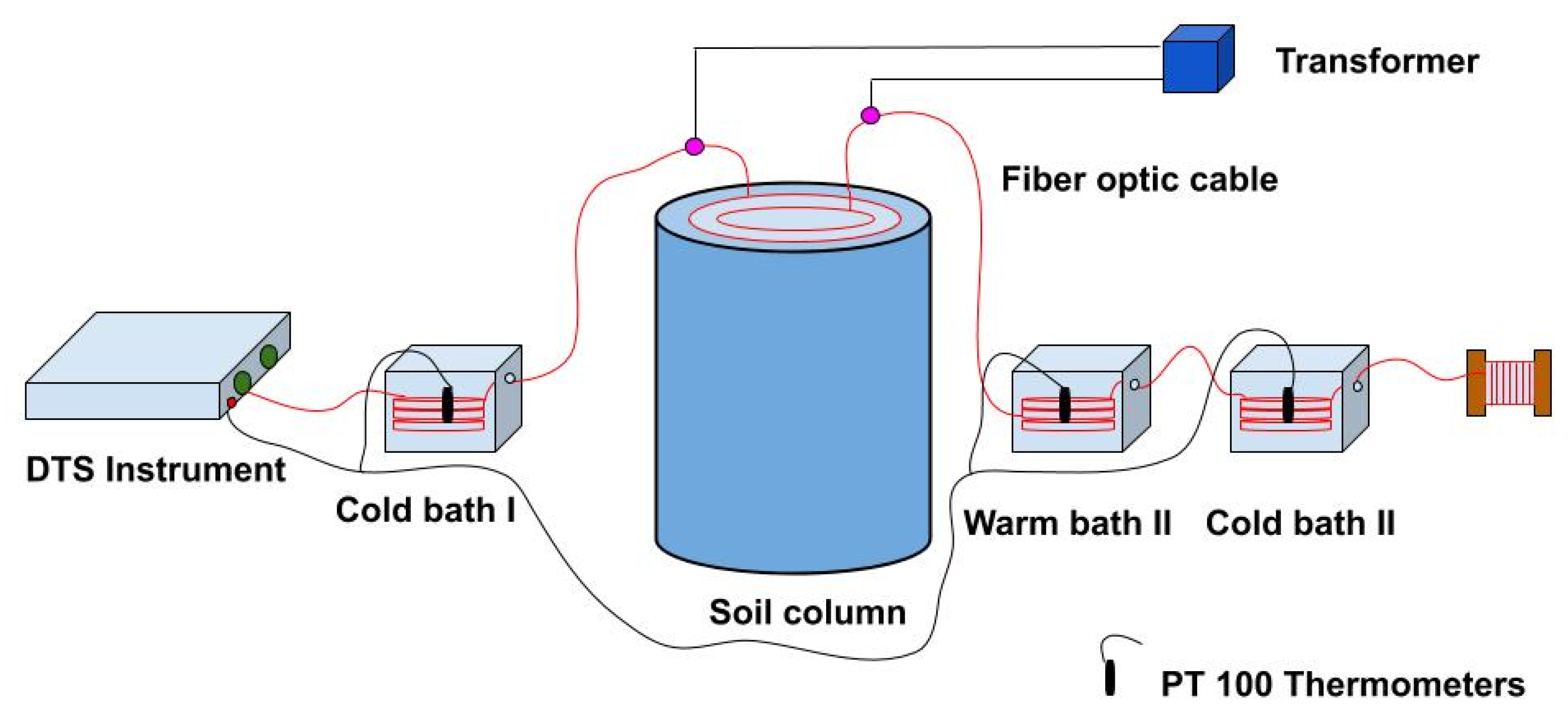
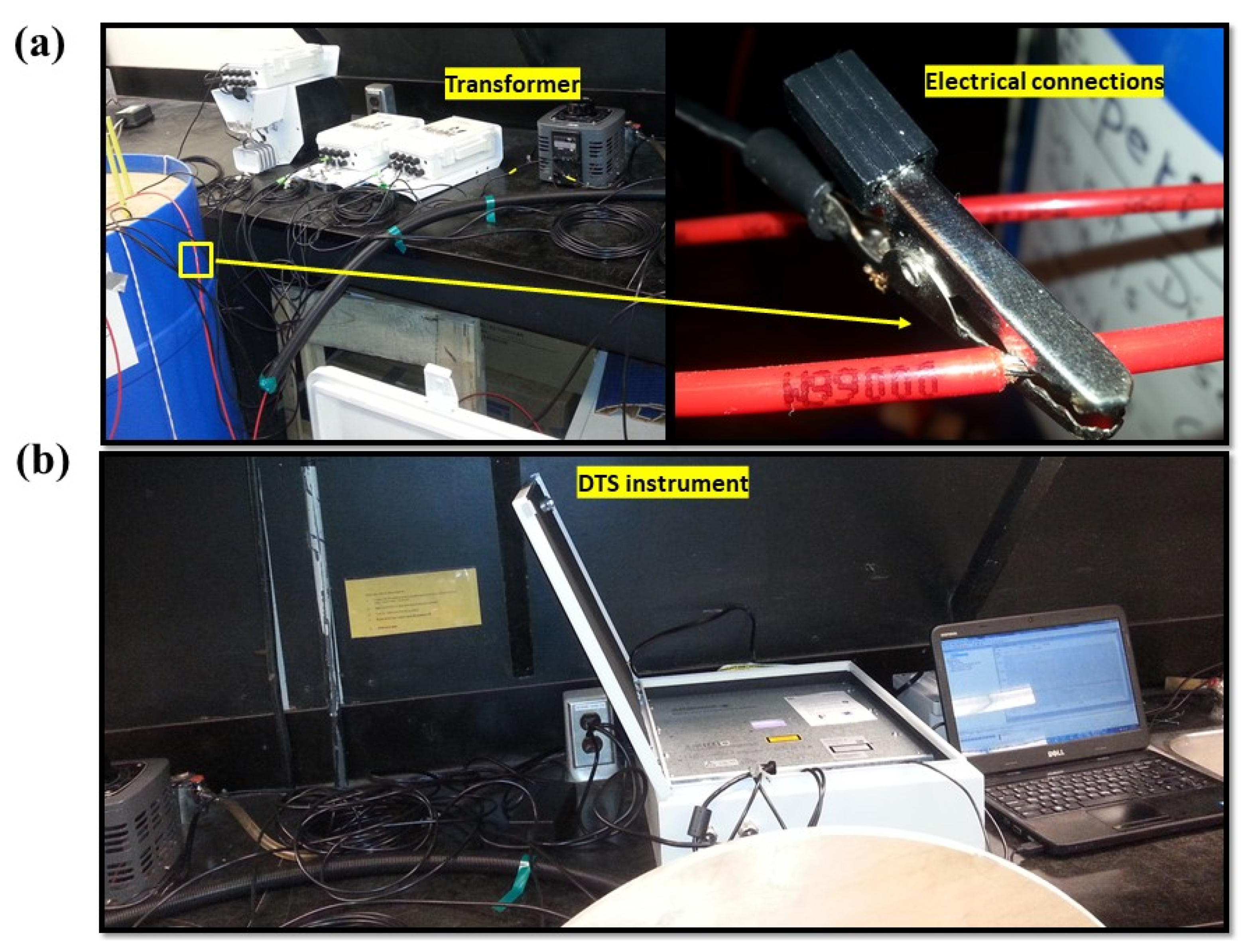
2.1. Soil Column Construction
2.2. Temperature Measurement
2.3. Heat Pulse Experiment
2.4. Data Analysis
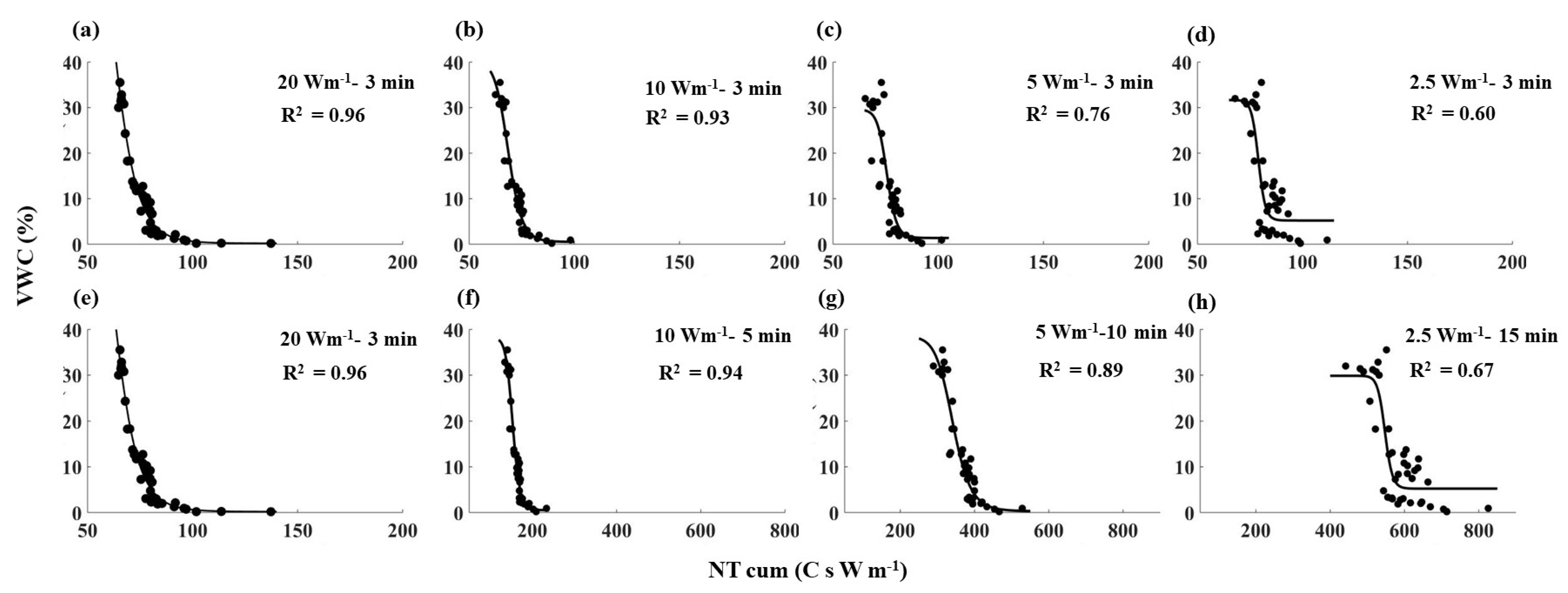
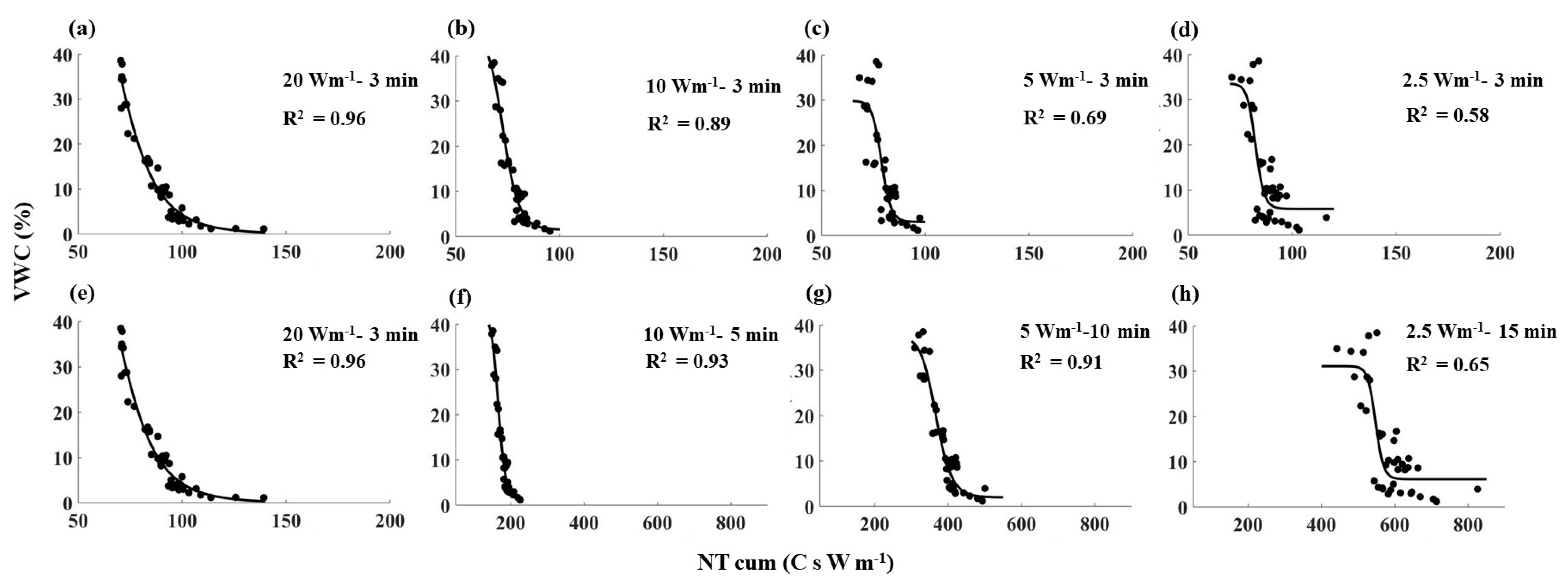
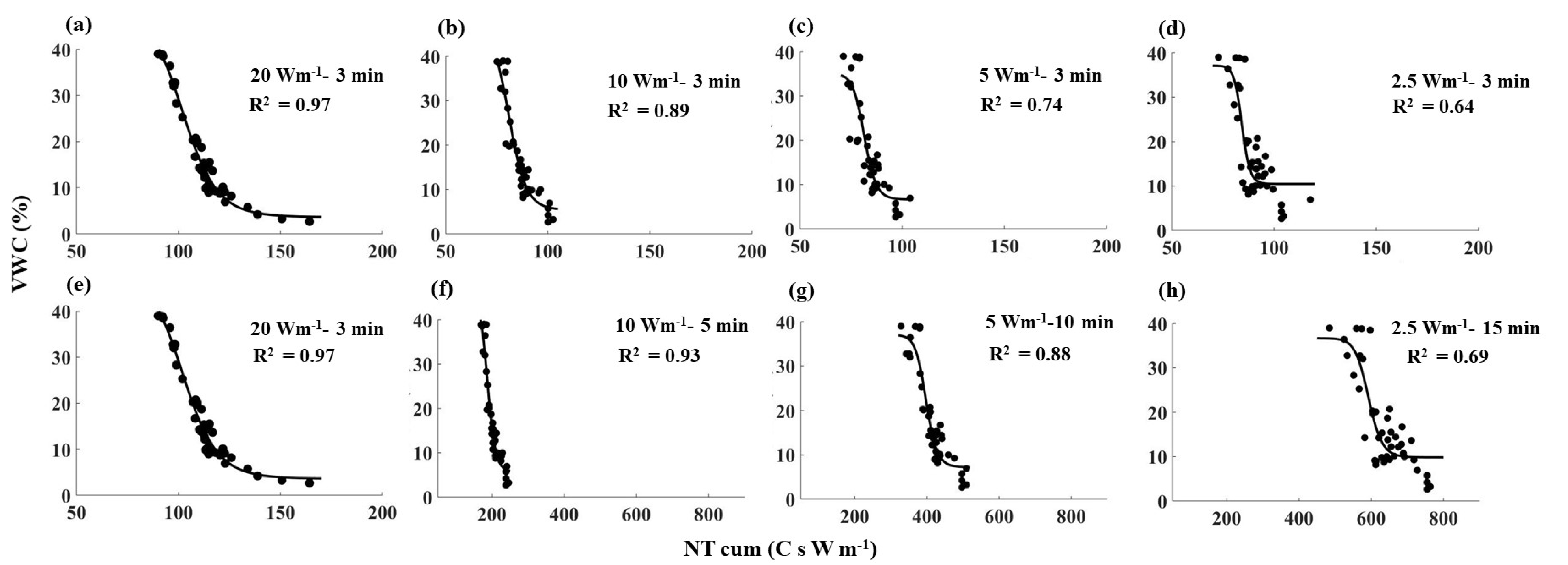
3. Results
3.1. Comparison of Tcum–SWC Relationships
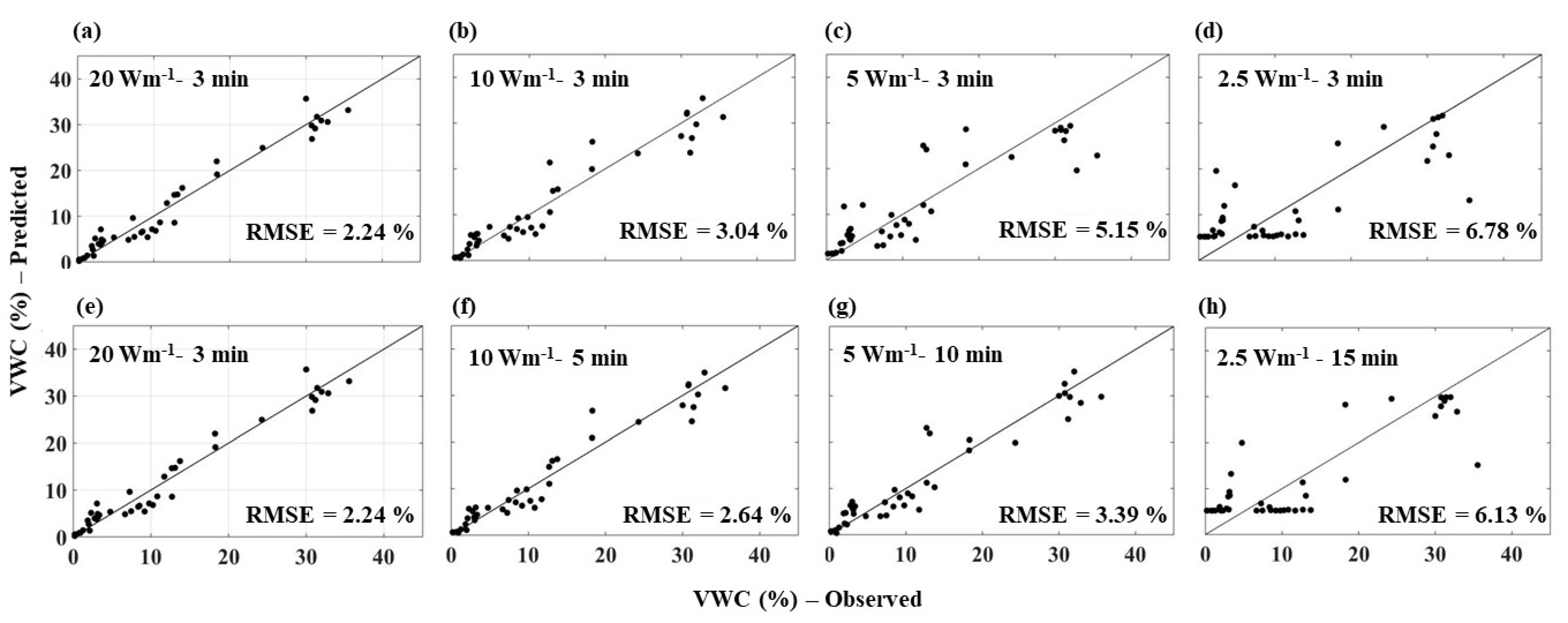
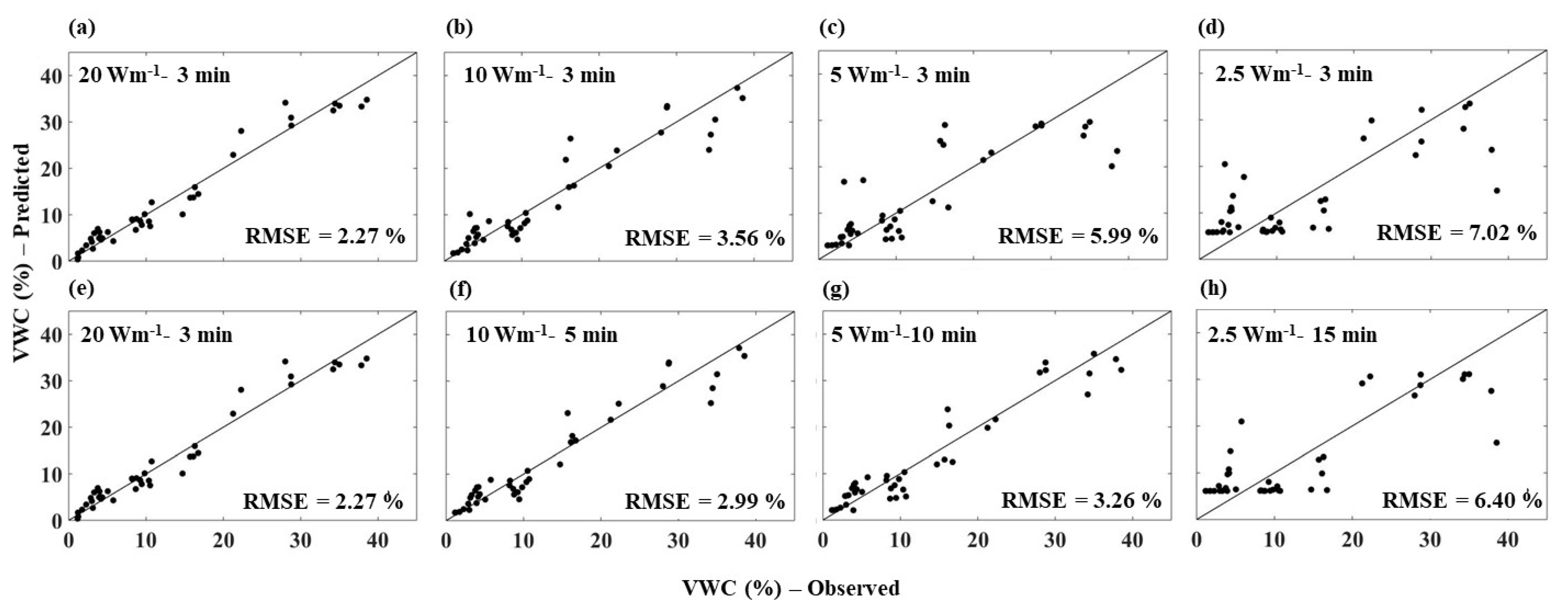
3.2. Comparison of Predicted Soil Water Content
4. Discussion
5. Conclusions
Author Contributions
Funding
Institutional Review Board Statement
Informed Consent Statement
Data Availability Statement
Acknowledgments
Conflicts of Interest
References
- Western, A.W.; Grayson, R.B.; Blöschl, G.; Willgoose, G.R.; McMahon, T.A. Observed spatial organization of soil moisture and its relation to terrain indices. Water Resour. Res. 1999, 35, 797–810. [Google Scholar] [CrossRef]
- Tallon, L.; Si, B. Representative soil water benchmarking for environmental monitoring. J. Environ. Inform. 2015, 4, 31–39. [Google Scholar] [CrossRef]
- Zreda, M.; Desilets, D.; Ferré, T.P.A.; Scott, R.L. Measuring soil moisture content non-invasively at intermediate spatial scale using cosmic-ray neutrons. Geophys. Res. Lett. 2008, 35, L21402. [Google Scholar] [CrossRef]
- Ragab, R.; Evans, J.G.; Battilani, A.; Solimando, D. The cosmic-ray soil moisture observation system (cosmos) for estimating the crop water requirement: New approach. Irrig. Drain. 2017, 66, 456–468. [Google Scholar] [CrossRef]
- Abdu, H.; Robinson, D.A.; Seyfried, M.; Jones, S.B. Geophysical imaging of watershed subsurface patterns and prediction of soil texture and water holding capacity. Water Resour. Res. 2008, 44, W00D18. [Google Scholar] [CrossRef]
- Moghadas, D.; Jadoon, K.Z.; McCabe, M.F. Spatiotemporal monitoring of soil water content profiles in an irrigated field using probabilistic inversion of time-lapse emi data. Adv. Water Resour. 2017, 110, 238–248. [Google Scholar] [CrossRef]
- Larson, K.M.; Small, E.E.; Gutmann, E.D.; Bilich, A.L.; Braun, J.J.; Zavorotny, V.U. Use of gps receivers as a soil moisture network for water cycle studies. Geophys. Res. Lett. 2008, 35, L24405. [Google Scholar] [CrossRef]
- Sayde, C.; Gregory, C.; Gil-Rodriguez, M.; Tufillaro, N.; Tyler, S.; van de Giesen, N.; English, M.; Cuenca, R.; Selker, J.S. Feasibility of soil moisture monitoring with heated fiber optics. Water Resour. Res. 2010, 46, W06201. [Google Scholar] [CrossRef]
- Steele‐Dunne, S.; Rutten, M.; Krzeminska, D.; Hausner, M.; Tyler, S.; Selker, J.; Bogaard, T.; Van de Giesen, N. Feasibility of soil moisture estimation using passive distributed temperature sensing. Water Resour. Res. 2010, 46, W03534. [Google Scholar] [CrossRef]
- Sayde, C.; Benitez Buelga, J.; Rodriguez-Sinobas, L.; El Khoury, L.; English, M.; van de Giesen, N.; Selker, J.S. Mapping variability of soil water content and flux across 1–1000 m scales using the Actively Heated Fiber Optic method. Water Resour. Res. 2014, 50, 7302–7317. [Google Scholar] [CrossRef]
- Gil-Rodríguez, M.; Rodríguez-Sinobas, L.; Benítez-Buelga, J.; Sánchez-Calvo, R. Application of active heat pulse method with fiber optic temperature sensing for estimation of wetting bulbs and water distribution in drip emitters. Agric. Water Manag. 2013, 120, 72–78. [Google Scholar] [CrossRef]
- Ciocca, F.; Lunati, I.; Van de Giesen, N.; Parlange, M.B. Heated Optical Fiber for Distributed Soil-Moisture Measurements: A Lysimeter Experiment. Vadose Zone J. 2012, 11. [Google Scholar] [CrossRef]
- Striegl, A.M.; Loheide, I.; Steven, P. Heated distributed temperature sensing for field scale soil moisture monitoring. Groundwater 2012, 50, 340–347. [Google Scholar] [CrossRef] [PubMed]
- Selker, J.; van de Giesen, N.; Westhoff, M.; Luxemburg, W.; Parlange, M.B. Fiber optics opens window on stream dynamics. Geophys. Res. Lett. 2006, 33, L24401. [Google Scholar] [CrossRef]
- Li, M.; Si, B.C.; Hu, W.; Dyck, M. Single-Probe Heat Pulse Method for Soil Water Content Determination: Comparison of Methods. Vadose Zone J. 2016, 15. [Google Scholar] [CrossRef]
- Dong, J.; Agliata, R.; Steele-Dunne, S.; Hoes, O.; Bogaard, T.; Greco, R.; Van de Giesen, N. The impacts of heating strategy on soil moisture estimation using actively heated fiber optics. Sensors 2017, 17, 2102. [Google Scholar] [CrossRef]
- Cao, D.; Fang, H.; Wang, F.; Zhu, H.; Sun, M. A Fiber Bragg-Grating-Based Miniature Sensor for the Fast Detection of Soil Moisture Profiles in Highway Slopes and Subgrades. Sensors 2018, 18, 4431. [Google Scholar] [CrossRef]
- Kurashima, T.; Horiguchi, T.; Tateda, M. Distributed-temperature sensing using stimulated Brillouin scattering in optical silica fibers. Opt. Lett. 1990, 15, 1038–1040. [Google Scholar] [CrossRef]
- Tyler, S.W.; Selker, J.S.; Hausner, M.B.; Hatch, C.E.; Torgersen, T.; Thodal, C.E.; Schladow, S.G. Environmental temperature sensing using Raman spectra DTS fiber—Optic methods. Water Resour. Res. 2009, 45. [Google Scholar] [CrossRef]
- Selker, J.S.; Thévenaz, L.; Huwald, H.; Mallet, A.; Luxemburg, W.; Van De Giesen, N.; Stejskal, M.; Zeman, J.; Westhoff, M.; Parlange, M.B. Distributed fiber—Optic temperature sensing for hydrologic systems. Water Resour. Res. 2006, 42. [Google Scholar] [CrossRef]
- Hausner, M.B.; Suárez, F.; Glander, K.E.; van de Giesen, N.; Selker, J.S.; Tyler, S.W. Calibrating single-ended fiber-optic Raman spectra distributed temperature sensing data. Sensors 2011, 11, 10859–10879. [Google Scholar] [CrossRef] [PubMed]


| Soil Type | Sand (%) | Silt (%) | Clay (%) | Bulk Density (Mg m−3) | Total Organic Carbon (%) |
|---|---|---|---|---|---|
| Sand | 100 | - | - | 1.65 | - |
| Sandy loam | 67 | 21 | 12 | 1.50 | 2.65 |
| Clay loam | 45 | 19 | 36 | 1.40 | 3.24 |
| Heating Strategy | 1 | 2 | 3 | 4 | 5 | 6 | 7 |
|---|---|---|---|---|---|---|---|
| Power intensity (W m−1) | 2.5 | 5 | 10 | 20 | 2.5 | 5 | 10 |
| Heating duration (min) | 3 | 3 | 3 | 3 | 15 | 10 | 5 |
Publisher’s Note: MDPI stays neutral with regard to jurisdictional claims in published maps and institutional affiliations. |
© 2021 by the authors. Licensee MDPI, Basel, Switzerland. This article is an open access article distributed under the terms and conditions of the Creative Commons Attribution (CC BY) license (http://creativecommons.org/licenses/by/4.0/).
Share and Cite
Vidana Gamage, D.N.; Vasava, H.B.; Strachan, I.B.; Adamchuk, V.I.; Biswas, A. Comparison of Heating Strategies on Soil Water Measurement Using Actively Heated Fiber Optics on Contrasting Textured Soils. Sensors 2021, 21, 962. https://doi.org/10.3390/s21030962
Vidana Gamage DN, Vasava HB, Strachan IB, Adamchuk VI, Biswas A. Comparison of Heating Strategies on Soil Water Measurement Using Actively Heated Fiber Optics on Contrasting Textured Soils. Sensors. 2021; 21(3):962. https://doi.org/10.3390/s21030962
Chicago/Turabian StyleVidana Gamage, Duminda N., Hiteshkumar B. Vasava, Ian B. Strachan, Viacheslav I. Adamchuk, and Asim Biswas. 2021. "Comparison of Heating Strategies on Soil Water Measurement Using Actively Heated Fiber Optics on Contrasting Textured Soils" Sensors 21, no. 3: 962. https://doi.org/10.3390/s21030962
APA StyleVidana Gamage, D. N., Vasava, H. B., Strachan, I. B., Adamchuk, V. I., & Biswas, A. (2021). Comparison of Heating Strategies on Soil Water Measurement Using Actively Heated Fiber Optics on Contrasting Textured Soils. Sensors, 21(3), 962. https://doi.org/10.3390/s21030962