Lightweight and Efficient Image Dehazing Network Guided by Transmission Estimation from Real-World Hazy Scenes

 , and
, and
Abstract
1. Introduction
- We propose a lightweight network, TGL-Net, based on a condensed residual encoder–decoder structure with skip connections for the fast dehazing of real-world images.
- To compute transmission errors without additional information for real-world hazy images, a reference transmission map is automatically estimated from a hazy image using a non-learning-based method F-DCP, which is a transmission-improved DCP method based on filters.
- A double-error loss function is introduced to combine the errors of a transmission map and dehazed output to supervise the training process of the network. With guidance from the proposed loss function, prior information is introduced into the model, yielding outputs with richer details and information.
- Both natural images and synthetic datasets are used for training the TGL-Net to make the model more applicable to real-world image dehazing and to achieve more rapid convergence during the training process.
2. Related Work
3. Proposed Method
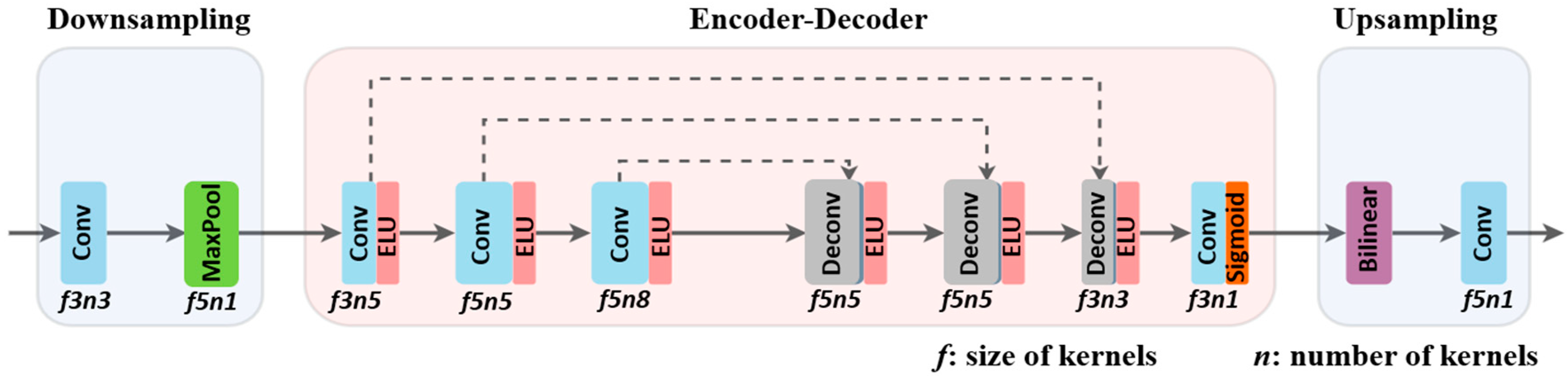
3.1. Architecture
3.1.1. Downsampling
3.1.2. Encoder–Decoder
3.1.3. Upsampling
3.2. Double Error Loss Function
3.3. Network Training
| Algorithm 1 Training algorithm |
| Set: the batch size the set of network parameters global atmospheric light error tolerance threshold Input: Sample hazy examples Sample haze-free examples 1: repeat 2: F-DCP(I), transmission map produced from F-DCP; 3: , transmission map produced from TGL-Net; 4: Calculate the using and by Equation (2); 5: Calculate by Equation (3); 6: Calculate the using and by Equation (4); 7: Bring and into Equation (5) to get ; 8: Update TGL-Net by descending the gradient of ; 9: until |
4. Experimental Results
4.1. Experimental Setting
4.1.1. Datasets
4.1.2. Implementation Details
4.1.3. Quality Measures
4.2. Comparisons
4.2.1. Evaluations on NTIRE Datasets
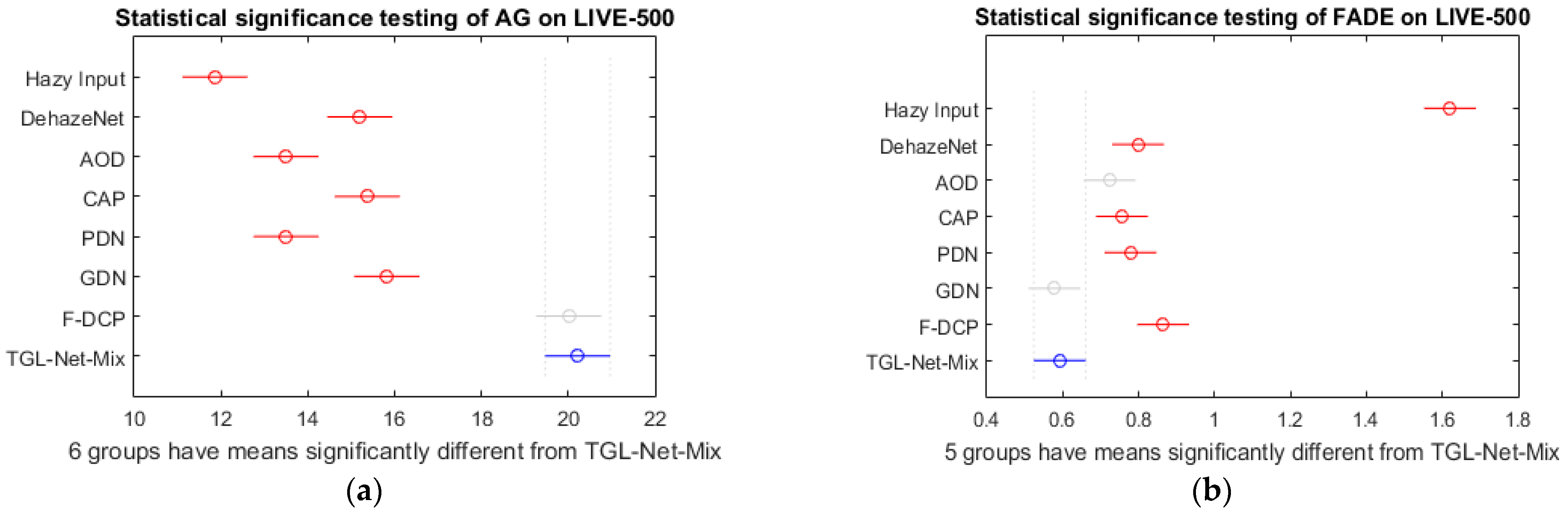
4.2.2. Evaluations on Other Datasets
4.2.3. Network Size and Efficiency
4.3. Ablation Study
4.3.1. Transmission Loss and Training Set
4.3.2. Downsampling and Upsampling
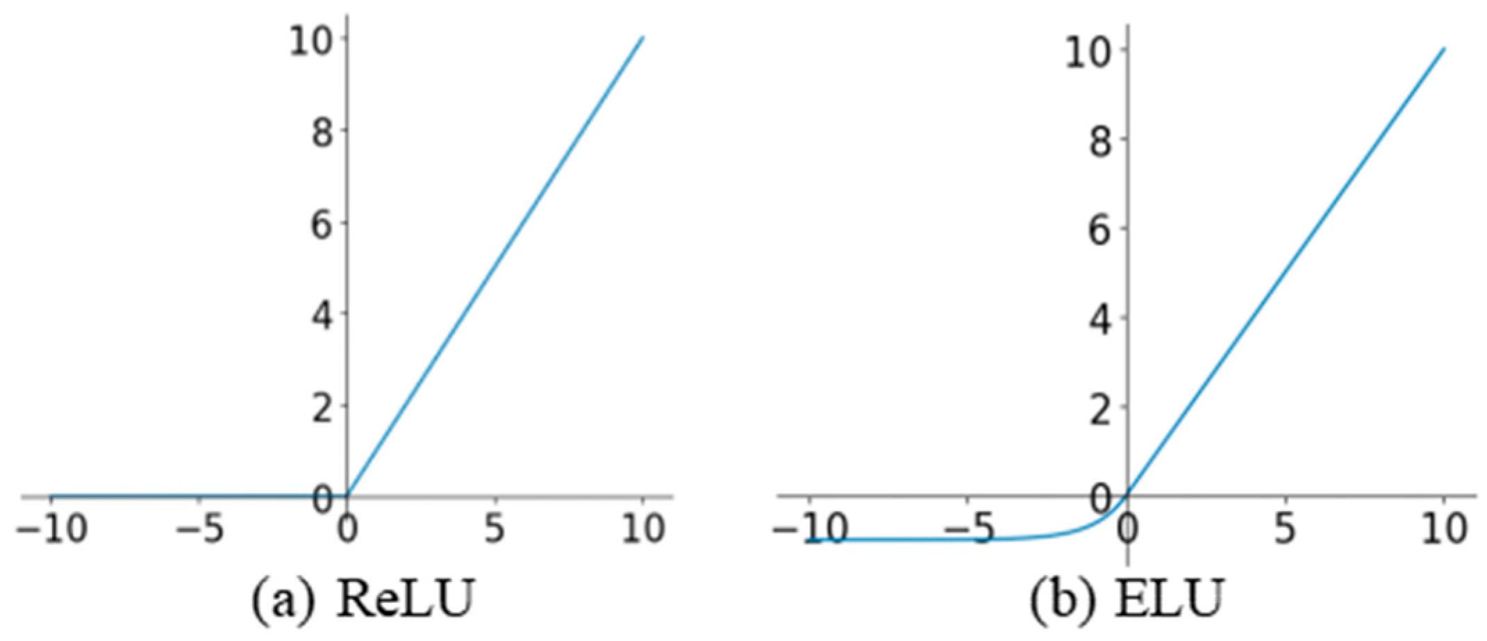
4.3.3. ReLU and ELU Activations
4.4. Transmission Map
4.5. Results on Images from Other Domains
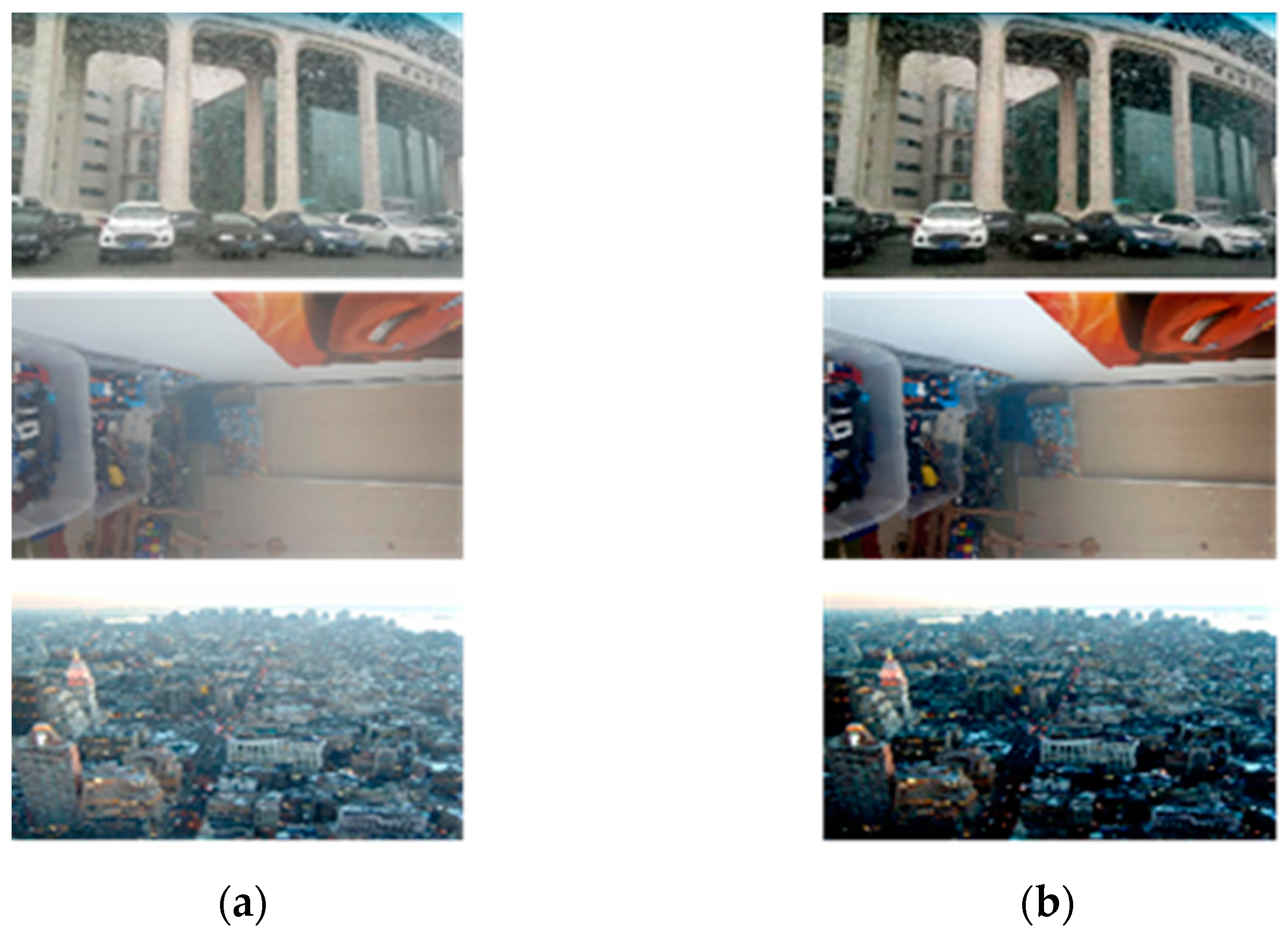
4.6. Results on Challenging Cases
5. Conclusions
Author Contributions
Funding
Institutional Review Board Statement
Informed Consent Statement
Data Availability Statement
Conflicts of Interest
References
- Narasimhan, S.G.; Nayar, S.K. Vision and the atmosphere. Int. J. Comput. Vis. 2002, 48, 233–254. [Google Scholar] [CrossRef]
- Zhu, Q.; Mai, J.; Shao, L. A fast single image haze removal algorithm using color attenuation prior. IEEE Trans. Image Process. 2015, 24, 3522–3533. [Google Scholar] [PubMed]
- Berman, D.; Avidan, S.; Treibitz, T. Non-local image dehazing. In Proceedings of the 2016 IEEE Conference on Computer Vision and Pattern Recognition (CVPR), Las Vegas, NV, USA, 27–30 June 2016; pp. 1674–1682. [Google Scholar]
- He, K.; Sun, J.; Tang, X. Single image haze removal using dark channel prior. IEEE Trans. Pattern Anal. Mach. Intell. 2011, 33, 2341–2353. [Google Scholar]
- Kopf, J.; Neubert, B.; Chen, B.; Cohen, M.; Cohen-Or, D.; Deussen, O.; Uyttendaele, M.; Lischinski, D. Deep photo: Model-based photograph enhancement and viewing. ACM Trans. Graph. 2018, 27, 116. [Google Scholar]
- Cai, B.; Xu, X.; Jia, K.; Qing, C.; Tao, D. Dehazenet: An end-to-end system for single image haze removal. IEEE Trans. Image Process. 2016, 25, 5187–5198. [Google Scholar] [CrossRef]
- Ren, W.; Liu, S.; Zhang, H.; Pan, J.; Cao, X.; Yang, M.H. Single image dehazing via multi-scale convolutional neural networks. In Proceedings of the 14th European Conference on Computer Vision, Amsterdam, The Netherlands, 8–16 October 2016. [Google Scholar]
- Li, B.; Peng, X.; Wang, Z.; Xu, J.; Feng, D. AOD-net: All in-one dehazing network. In Proceedings of the 2017 IEEE International Conference on Computer Vision, Venice, Italy, 22–29 October 2017; pp. 4770–4778. [Google Scholar]
- Engin, D.; Genc, A.; Ekenel, H.K. Cycle-Dehaze: Enhanced CycleGAN for single image dehazing. In Proceedings of the IEEE Conference on Computer Vision and Pattern Recognition Workshops, CVPR Workshops 2018, Salt Lake City, UT, USA, 18–22 June 2018; pp. 825–833. [Google Scholar]
- Yang, D.; Sun, J. Proximal dehaze-net: A prior learning-based deep network for single image dehazing. In Proceedings of the ECCV 2018, Munich, Germany, 8–14 September 2018; pp. 702–717. [Google Scholar]
- Liu, X.; Ma, Y.; Shi, Z.; Chen, J. GridDehazeNet: Attention-based multi-scale network for image dehazing. In Proceedings of the International Conference on Computer Vision, Seoul, Korea, 27 October–2 November 2019; pp. 7314–7323. [Google Scholar]
- Chen, W.; Ding, J.; Kuo, S. PMS-Net: Robust haze removal based on patch map for single images. In Proceedings of the CVPR, Long Beach, CA, USA, 16–20 June 2019; pp. 11681–11689. [Google Scholar]
- Zhang, H.; Sindagi, V.; Patel, V.M. Joint transmission map estimation and dehazing using deep networks. IEEE Trans. Circuits Syst. Video Technol. 2020, 30, 1975–1986. [Google Scholar] [CrossRef]
- Li, L.; Dong, Y.; Ren, W.; Pan, J.; Gao, C.; Sang, N.; Yang, M.H. Semi-supervised image dehazing. IEEE Trans. Image Process. 2020, 29, 2766–2779. [Google Scholar] [CrossRef]
- Chen, Y.; Li, Z.; Bhanu, B.; Tang, D.; Peng, Q.; Zhang, Q. Improve transmission by designing filters for image dehazing. In Proceedings of the 2018 IEEE 3rd International Conference on Image, Vision and Computing (ICIVC 2018), Chongqing, China, 27–29 June 2018; pp. 374–378. [Google Scholar]
- Kim, T.K.; Paik, J.K.; Kang, B.S. Contrast enhancement system using spatially adaptive histogram equalization with temporal filtering. IEEE Trans. Consum. Electron. 1998, 44, 82–87. [Google Scholar]
- Lucchese, L.; Mitra, S.K.; Mukherjee, J. A new algorithm based on saturation and desaturation in the xy chromaticity diagram for enhancement and re-rendition of color images. In Proceedings of the 2001 International Conference on Image Processing, Thessaloniki, Greece, 7–10 October 2001; pp. 1077–1080. [Google Scholar]
- Tan, R.T. Visibility in bad weather from a single image. In Proceedings of the 2008 IEEE Conference on Computer Vision and Pattern Recognition, Anchorage, AK, USA, 23–28 June 2008; pp. 24–26. [Google Scholar]
- Meng, G.; Wang, Y.; Duan, J.; Xiang, S.; Pan, C. Efficient image dehazing with boundary constraint and contextual regularization. In Proceedings of the ICCV—IEEE International Conference on Computer Vision, Sydney, Australia, 1–8 December 2013; pp. 617–624. [Google Scholar]
- Fattal, R. Dehazing using color-lines. ACM Trans. Graph. 2014, 34, 1–14. [Google Scholar] [CrossRef]
- Silberman, N.; Hoiem, D.; Kohli, P.; Fergus, R. Indoor segmentation and support inference from RGB images. In Proceedings of the 12th European Conference on Computer Vision, Florence, Italy, 7–13 October 2012; pp. 746–760. [Google Scholar]
- Scharstein, D.; Hirschmüller, H.; Kitajima, Y.; Krathwohl, G.; Nešić, N.; Wang, X.; Westling, P. High-resolution stereo datasets with subpixel-accurate ground truth. In Proceedings of the 36th German Conference on Pattern Recognition Münster, 2–5 September 2014; pp. 31–42. [Google Scholar]
- Li, B.; Ren, W.; Fu, D.; Tao, D.; Feng, D.; Zeng, W.; Wang, Z. Benchmarking single image dehazing and beyond. IEEE Trans. Image Process. 2019, 28, 492–505. [Google Scholar] [CrossRef]
- Ancuti, C.O.; Ancuti, C.; Timofte, R.; Vleeschouwer, C.D. I-HAZE: A dehazing benchmark with real hazy and haze-free indoor images. In Proceedings of the Advanced Concepts for Intelligent Vision Systems, Espace Mendes France, Poitiers, France, 24–27 September 2018; pp. 620–631. [Google Scholar]
- Ancuti, C.O.; Ancuti, C.; Timofte, R.; Vleeschouwer, C.D. O-HAZE: A dehazing benchmark with real hazy and haze-free outdoor images. In Proceedings of the 2018 IEEE Conference on Computer Vision and Pattern Recognition Workshops, CVPR Workshops 2018, Salt Lake City, UT, USA, 18–22 June 2018; pp. 754–762. [Google Scholar]
- Ancuti, C.O.; Ancuti, C.; Sbert, M.; Timofte, R. Dense haze: A benchmark for image dehazing with dense-haze and haze-free images. arXiv 2019, arXiv:1904.02904. [Google Scholar]
- Mao, X.; Shen, C.; Yang, Y. Image restoration using very deep convolutional encoder-decoder networks with symmetric skip connections. In Proceedings of the 30th International Conference on Neural Information Processing Systems, Barcelona, Spain, 5–10 December 2016; pp. 2802–2810. [Google Scholar]
- He, K.; Zhang, X.; Ren, S.; Sun, J. Deep residual learning for image recognition. In Proceedings of the 2016 IEEE Conference on Computer Vision and Pattern Recognition (CVPR), Las Vegas, NV, USA, 27–30 June 2016; pp. 770–778. [Google Scholar]
- Glorot, X.; Bengio, Y. Understanding the difficulty of training deep feedforward neural networks. In Proceedings of the AIS Conference, Sardinia, Italy, 13–15 May 2010; pp. 249–256. [Google Scholar]
- Clevert, D.A.; Unterthiner, T.; Hochreiter, S. Fast and accurate deep network learning by exponential linear units (ELUs). In Proceedings of the International Conference on Learning Representations, San Juan, Puerto Rico, 12–19 November 2019. [Google Scholar]
- Ancuti, C.; Ancuti, C.O.; Timofte, R. NTIRE 2018 challenge on image dehazing: Methods and results. In Proceedings of the IEEE Conference on Computer Vision and Pattern Recognition Workshops, CVPR Workshops 2018, Salt Lake City, UT, USA, 18–22 June 2018; pp. 891–901. [Google Scholar]
- Galdran, A.; Alvarez-Gila, A.; Bria, A.; Vazquez-Corral, J.; Bertalmío, M. On the duality between retinex and image dehazing. In Proceedings of the IEEE Conference on Computer Vision and Pattern Recognition Workshops, CVPR Workshops 2018, Salt Lake City, UT, USA, 18–22 June 2018; pp. 8212–8221. [Google Scholar]
- Choi, L.K.; You, J.; Bovik, A.C. Referenceless prediction of perceptual fog density and perceptual image defogging. IEEE Trans. Image Process. 2015, 24, 3888–3901. [Google Scholar] [CrossRef] [PubMed]
- Zhang, H.; Sindagi, V.; Patel, V.M. Multi-scale single image dehazing using perceptual pyramid deep network. In Proceedings of the IEEE Conference on Computer Vision and Pattern Recognition Workshops, CVPR Workshops 2018, Salt Lake City, UT, USA, 18–22 June 2018; pp. 902–911. [Google Scholar]
- Liu, Y.; Yang, H.; Gao, S.; Yang, K.; Yang, K. Criteria to evaluate the fidelity of image enhancement by MSRCR. IET Image Process. 2018, 12, 880–887. [Google Scholar] [CrossRef]
- Gu, K.; Tao, D.; Qiao, J.F.; Lin, W. Learning a no-reference quality assessment model of enhanced images with big data. IEEE Trans. Neural Netw. Learn. Syst. 2018, 29, 1301–1313. [Google Scholar] [CrossRef] [PubMed]
- Ying, Z.; Niu, H.; Gupta, P.; Mahajan, D.; Ghadiyaram, D.; Bovik, A. From patches to pictures (PaQ-2-PiQ): Mapping the perceptual space of picture quality. In Proceedings of the IEEE Conference on Computer Vision and Pattern Recognition Workshops, CVPR, Seattle, WA, USA, 14–19 June 2020; pp. 3575–3585. [Google Scholar]
- Yang, H.; Pan, J.; Yan, Q.; Sun, W.; Ren, J.; Tai, Y. Image dehazing using bilinear composition loss function. arXiv 2017, arXiv:1710.00279. [Google Scholar]


| Dehaze Network | Ours | DehazeNet | AOD | Cycle | PDN | GDN | PMS-Net | Joint-GAN | SSID |
|---|---|---|---|---|---|---|---|---|---|
| Published in | -- | TIP | ICCV | CVPR | ECCV | ECCV | CVPR | TCSVT | TIP |
| Published year | 2021 | 2016 | 2017 | 2018 | 2018 | 2019 | 2019 | 2020 | 2020 |
| Reference No. | -- | [6] | [8] | [9] | [10] | [11] | [12] | [13] | [14] |
| Symmetrical structure | ✓ | x | x | x | x | ✓ | x | ✓ | ✓ |
| Skip connection | ✓ | x | partly | partly | x | partly | partly | ✓ | ✓ |
| Transmission loss | ✓ | ✓ | x | x | ✓ | x | x | ✓ | x |
| Transmission-guided | ✓ | ✓ | x | x | ✓ | x | ✓ | ✓ | x |
| Estimate transmission from real-world images | ✓ | x | x | x | x | x | x | x | x |
| Training on real-world images | ✓ | x | x | ✓ | x | x | x | x | ✓ |
| Training on synthetic images | ✓ | ✓ | ✓ | ✓ | ✓ | ✓ | ✓ | ✓ | ✓ |
| Lightweight (compared to AOD) | ✓ rank 2 | ✓ rank 3 | ✓ rank 1 | x | x | x | x | x | x |
| Efficient (comparable to AOD) | ✓ rank 1 | x | ✓ rank 2 | x | x | x | x | ✓ rank 3 | x |
| Network Phase | Type | Input Size h × w × c | Kernels f × f × n |
|---|---|---|---|
| Downsampling | Conv | 480 × 640 × 3 | 3 × 3 × 3 |
| MaxPool | 480 × 640 × 3 | 5 × 5 × 1 | |
| Encoder– Decoder | Conv | 96 × 128 × 3 | 3 × 3 × 5 |
| 96 × 128 × 5 | 5 × 5 × 5 | ||
| 96 × 128 × 5 | 5 × 5 × 8 | ||
| Deconv | 96 × 128 × 8 | 5 × 5 × 5 | |
| 96 × 128 × 5 | 5 × 5 × 5 | ||
| 96 × 128 × 5 | 3 × 3 × 3 | ||
| Conv | 96 × 128 × 3 | 3 × 3 ×1 | |
| Upsampling | Bilinear | 96 × 128 × 1 | - |
| Conv | 480 × 640 × 1 | 5 × 5 × 1 |
| Method/Input | NTIRE18Val-10 | NTIRE18Train-60 | ||
|---|---|---|---|---|
| PSNR | SSIM | PSNR | SSIM | |
| Hazy Input | 13.683 | 0.664 | 14.243 | 0.660 |
| DehazeNet [6] | 14.042 | 0.638 | 14.521 | 0.640 |
| AOD [8] | 15.161 | 0.656 | 15.550 | 0.652 |
| F-DCP [15] | 14.863 | 0.676 | 15.171 | 0.665 |
| TGL-Net-Syn | 15.164 | 0.650 | 15.462 | 0.626 |
| TGL-Net-Mix | 15.480 | 0.659 | - | - |
| Method/Input | NTIRE18-20 | NTIRE19-10 | ||||||||
|---|---|---|---|---|---|---|---|---|---|---|
| AG | IE | FADE | BIQME | PaQ2PiQ | AG | IE | FADE | BIQME | PaQ2PiQ | |
| Hazy Input | 4.17 | 1.77 | 2.81 | 0.45 | 65.30 | 0.93 | 0.92 | 5.91 | 0.35 | 61.86 |
| DehazeNet [6] | 5.92 | 2.24 | 1.11 | 0.53 | 64.91 | 1.36 | 1.42 | 3.28 | 0.36 | 62.93 |
| AOD [8] | 5.55 | 2.24 | 1.13 | 0.53 | 63.08 | 2.07 | 1.90 | 1.17 | 0.47 | 60.74 |
| Cycle [9] | 5.06 | 3.78 | 1.65 | 0.43 | 69.27 | 0.93 | 0.84 | 5.83 | 0.36 | 60.67 |
| F-DCP [15] | 8.69 | 3.32 | 1.02 | 0.60 | 67.05 | 3.04 | 1.62 | 4.39 | 0.39 | 65.59 |
| TGL-Net-Mix | 9.19 | 2.62 | 0.92 | 0.59 | 65.94 | 3.29 | 1.81 | 2.56 | 0.41 | 66.79 |
| Method/Input | LIVE-500 | Internet-48 | ||||||||
|---|---|---|---|---|---|---|---|---|---|---|
| AG | IE | FADE | BIQME | PiQ2PaQ | AG | IE | FADE | BIQME | PiQ2PaQ | |
| Hazy Input | 11.86 | 6.65 | 1.62 | 0.51 | 68.70 | 9.20 | 5.04 | 2.06 | 0.48 | 68.14 |
| DehazeNet [6] | 15.20 | 7.91 | 0.80 | 0.56 | 67.96 | 12.32 | 6.13 | 0.99 | 0.56 | 68.29 |
| AOD [8] | 13.50 | 8.53 | 0.72 | 0.56 | 66.76 | 11.04 | 6.21 | 0.99 | 0.54 | 67.77 |
| CAP [2] | 15.37 | 6.63 | 0.76 | 0.55 | 67.46 | 13.14 | 5.20 | 0.94 | 0.55 | 67.77 |
| PDN [10] | 13.50 | 8.17 | 0.78 | 0.58 | 68.25 | 12.66 | 6.92 | 0.83 | 0.59 | 68.35 |
| GDN [11] | 15.82 | 7.81 | 0.58 | 0.54 | 67.19 | 12.38 | 6.72 | 0.75 | 0.56 | 67.59 |
| F-DCP [15] | 20.01 | 11.08 | 0.87 | 0.59 | 69.75 | 16.92 | 8.49 | 1.04 | 0.58 | 68.77 |
| TGL-Net-Mix | 20.22 | 7.88 | 0.59 | 0.54 | 68.13 | 15.93 | 6.29 | 0.91 | 0.54 | 68.40 |
| Models | DehazeNet [6] | AOD [8] | Bilinear-Net [38] | PMS-Net [12] | Joint-GAN [13] | RED-Net20 [21] | RED-Net30 [21] | TGL-Net (Ours) |
|---|---|---|---|---|---|---|---|---|
| Parameters | 8.11 K | 1.71 K | 298.81 K | 20.77 M | 3.32 M | 0.64 M | 0.99 M | 3.57 K |
| Models | DehazeNet [6] | AOD [8] | CAP [2] | PDN [12] | GDN [13] | F-DCP [15] | TGL-Net |
|---|---|---|---|---|---|---|---|
| LIVE-500 | 3.362 | 0.609 | 0.928 | 3.541 | 10.726 | 0.815 | 0.088 |
| Internet-48 | 3.438 | 0.599 | 1.177 | 4.059 | 13.873 | 0.983 | 0.087 |
| Models | DehazeNet [6] | AOD [8] | TGL-Net |
|---|---|---|---|
| NTIRE 2018 | 47.50 | 1.14 | 0.046 |
| Models | Transmission Loss Guided? | Training Set | PSNR on NTIRE18Val-10 |
|---|---|---|---|
| L-Net-Mix | x | A + B | 15.40 |
| TGL-Net-Syn | ✓ | Only A | 15.16 |
| TGL-Net-Mix | ✓ | A + B | 15.48 |
| Method | NTIRE18-20 | Internet-48 | NTIRE19-10 |
|---|---|---|---|
| L-Net-Mix | 4.77 | 10.93 | 1.73 |
| TGL-Net-Mix | 9.19 | 16.05 | 3.29 |
| Network Model | TGL-Net-Mix | TGL-ResFix | ||
|---|---|---|---|---|
| Resolution of Input Image | 2048 × 2048 | 3840 × 3840 | 2048 × 2048 | 3840 × 3840 |
| Computations (GFLOPs) | 2.09 | 7.38 | 30.79 | 108.26 |
| Run time (s) | 0.89 | 2.69 | 4.15 | 15.32 |
| CPU utilization (%) | 13.5 | 19.9 | 20.5 | 35.7 |
Publisher’s Note: MDPI stays neutral with regard to jurisdictional claims in published maps and institutional affiliations. |
© 2021 by the authors. Licensee MDPI, Basel, Switzerland. This article is an open access article distributed under the terms and conditions of the Creative Commons Attribution (CC BY) license (http://creativecommons.org/licenses/by/4.0/).
Share and Cite
Li, Z.; Zhang, J.; Zhong, R.; Bhanu, B.; Chen, Y.; Zhang, Q.; Tang, H. Lightweight and Efficient Image Dehazing Network Guided by Transmission Estimation from Real-World Hazy Scenes. Sensors 2021, 21, 960. https://doi.org/10.3390/s21030960
Li Z, Zhang J, Zhong R, Bhanu B, Chen Y, Zhang Q, Tang H. Lightweight and Efficient Image Dehazing Network Guided by Transmission Estimation from Real-World Hazy Scenes. Sensors. 2021; 21(3):960. https://doi.org/10.3390/s21030960
Chicago/Turabian StyleLi, Zhan, Jianhang Zhang, Ruibin Zhong, Bir Bhanu, Yuling Chen, Qingfeng Zhang, and Haoqing Tang. 2021. "Lightweight and Efficient Image Dehazing Network Guided by Transmission Estimation from Real-World Hazy Scenes" Sensors 21, no. 3: 960. https://doi.org/10.3390/s21030960
APA StyleLi, Z., Zhang, J., Zhong, R., Bhanu, B., Chen, Y., Zhang, Q., & Tang, H. (2021). Lightweight and Efficient Image Dehazing Network Guided by Transmission Estimation from Real-World Hazy Scenes. Sensors, 21(3), 960. https://doi.org/10.3390/s21030960