
A Machine Learning Multi-Class Approach for Fall Detection Systems Based on Wearable Sensors with a Study on Sampling Rates Selection †


Abstract
1. Introduction
- RQ1:
- What is the difference in performance across various types of Machine Learning (ML) algorithms in a FDS?To answer this, we developed a reliable FDS by the mean of wearable sensors (accelerometer and gyroscope) and ML algorithms. The goal is to compare lazy, eager and ensemble learning algorithms and assess their results. We implemented five algorithms and tested them in the same setup.
- RQ2:
- What is the effect of the sensors’ sampling rate on the fall detection?To study this, we analyzed the influence of the sensors’ sampling rate on the detection. We filtered the data in order to reduce the number of samples measured per second. We then experimented on the filtered data with five ML algorithms. This research question extends our previous work [8].
- RQ3:
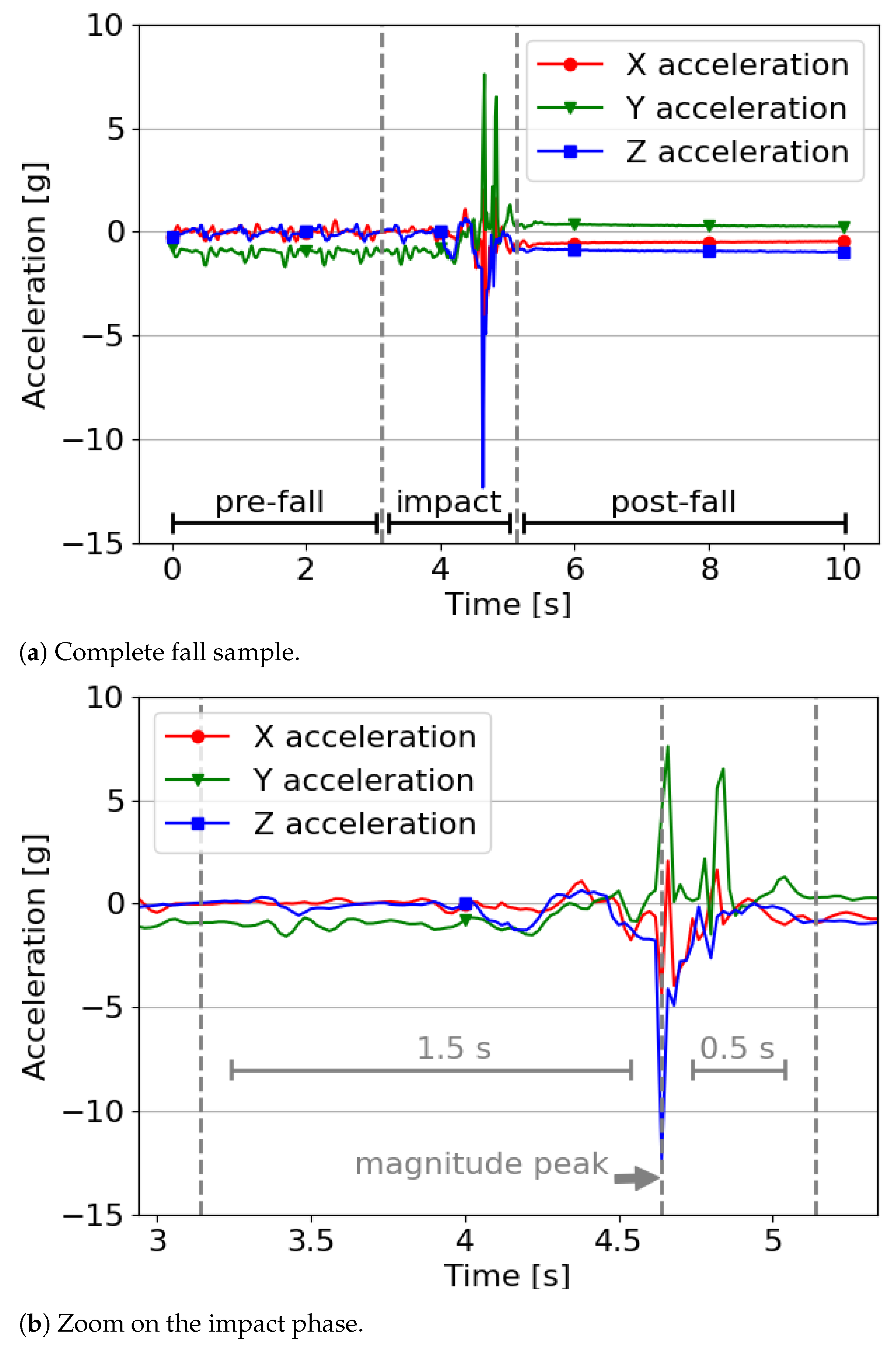
- What is the difference in performance across various types of ML algorithms by adopting a multi-class approach for identifying phases of a fall?We experimented a different fall detection approach where falls are split into three phases. These are: the period before the fall happens (pre-fall), the fall itself (impact) and after the fall happened (post-fall). This research question extends our previous work [8].
2. Related Work
2.1. Choice of Sensors and Sampling Rate
2.2. Sensing Position
2.3. Algorithms
2.4. Classification Strategies
2.5. Strengths and Weaknesses
3. Materials and Methods
3.1. Dataset
3.2. Data Preprocessing
- From 5 to 15 s.
- From 25 to 35 s.
- From 45 to 55 s.
- From 65 to 75 s.
- From 85 to 95 s.
3.3. Feature Extraction
3.4. Classification Algorithms
3.4.1. k-Nearest Neighbor (KNN)
3.4.2. Support Vector Machines (SVM)
- C makes a compromise between the number of misclassified instances and the margins width of the hyperplane. The lower the value, the larger the margins but potentially increasing the number of errors. When the margins are thin, the number of misclassified samples is low, but this can lead to overfitting.
- Kernel changes the employed mathematical function which creates the hyperplane. A typically used kernel is the Radial Basis Function.
- Gamma defines the influence that one data has compared to the other ones. The higher the value, the bigger its influence range, but this can lead to overfitting. With a low value, the model is at risk of underfitting.
3.4.3. Decision Tree (DT)
- Criterion is the function allowing to measure the quality of the split of a node. A commonly used criterion is Gini impurity.
- Splitter is the split selection method of each node because there may be several split solutions. A commonly used splitter is the best split.
- Max depth defines the maximum depth that a tree can reach during its creation. A big depth complicates the structure and tends to create overfitting on the data. But on the contrary, a low depth tends to create underfitting.
- Min samples split is the minimum number of data required to enable the split of a node. This value is usually low because the higher it is, the more constrained the model becomes, which creates underfitting.
- Min samples leaf is the minimum number of data required to consider a node as a leaf. Its effect is similar to the previous parameter because a high value would create underfitting.
- Max features corresponds to the maximum number of features to take into account when the algorithm searches for the best split. This hyper-parameter depends on the employed data but also tends to produce overfitting when its value is high.
3.4.4. Random Forest (RF)
3.4.5. Gradient Boosting (GB)
- Loss defines the loss function which must be optimized.
- Learning rate slows the learning speed of the algorithm by reducing the contribution that each tree produces. This avoids to rapidly create overfitting.
- Estimator corresponds to the number of sequential DTs. A high number would produce good results but a number too high may create an overfitting issue and use more computational power and memory. The idea is to make a compromise between the number of estimators and the learning rate.
- Subsample defines the data fraction used to train each tree. When the fraction is smaller than 1, the model becomes a Stochastic GB algorithm which reduces the variance but increases the bias.
3.5. Evaluation
- True negative (TN): Correct classification of a negative condition, meaning a reject.
- False positive (FP): Incorrect classification of a negative condition, meaning a false alarm.
- False negative (FN): Incorrect classification of a positive condition, meaning a missed.
- True positive (TP): Correct classification of a positive condition, meaning a hit.
3.6. Multi-Class Approach Considerations
4. Results and Discussion
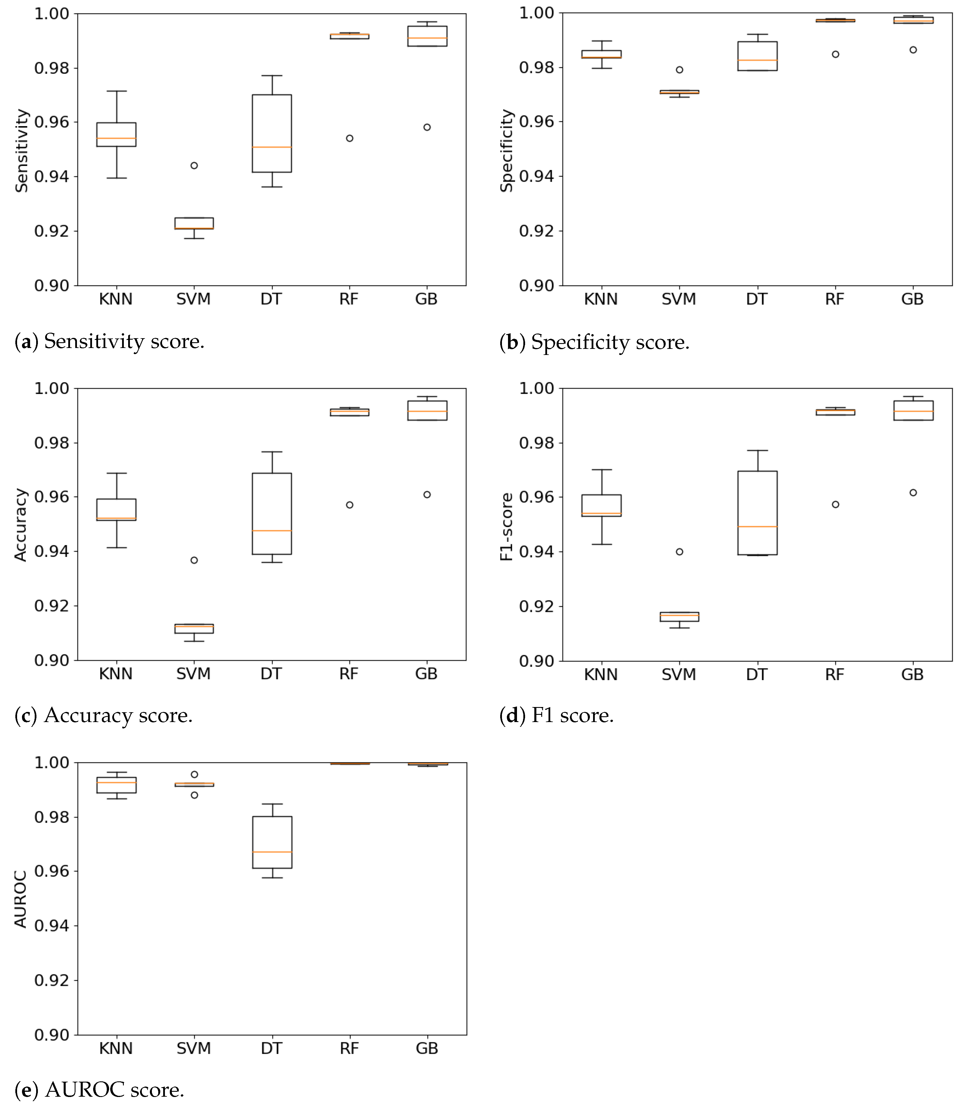
4.1. Fall Detection System (FDS) Performance
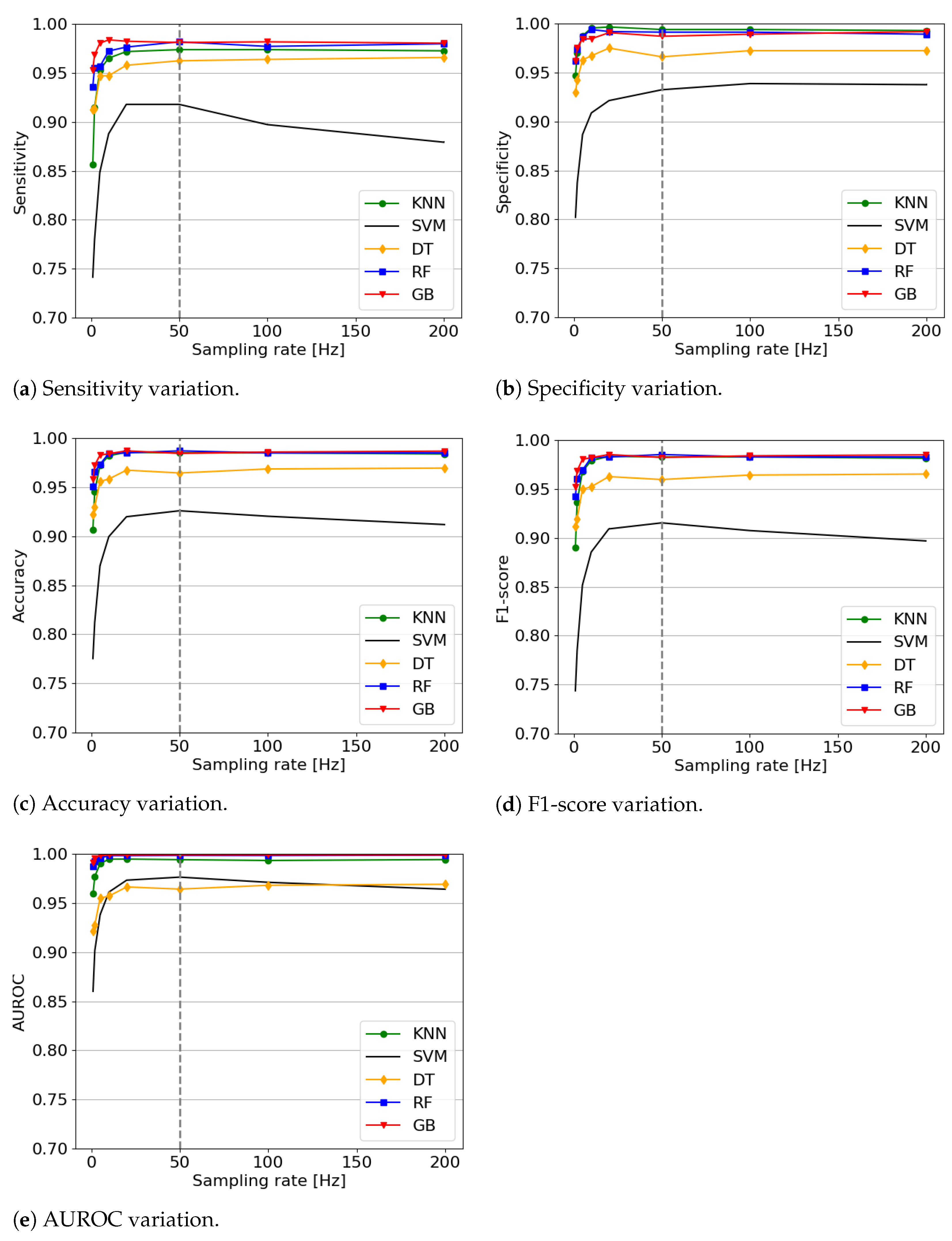
4.2. Sensors’ Sampling Rate Effect
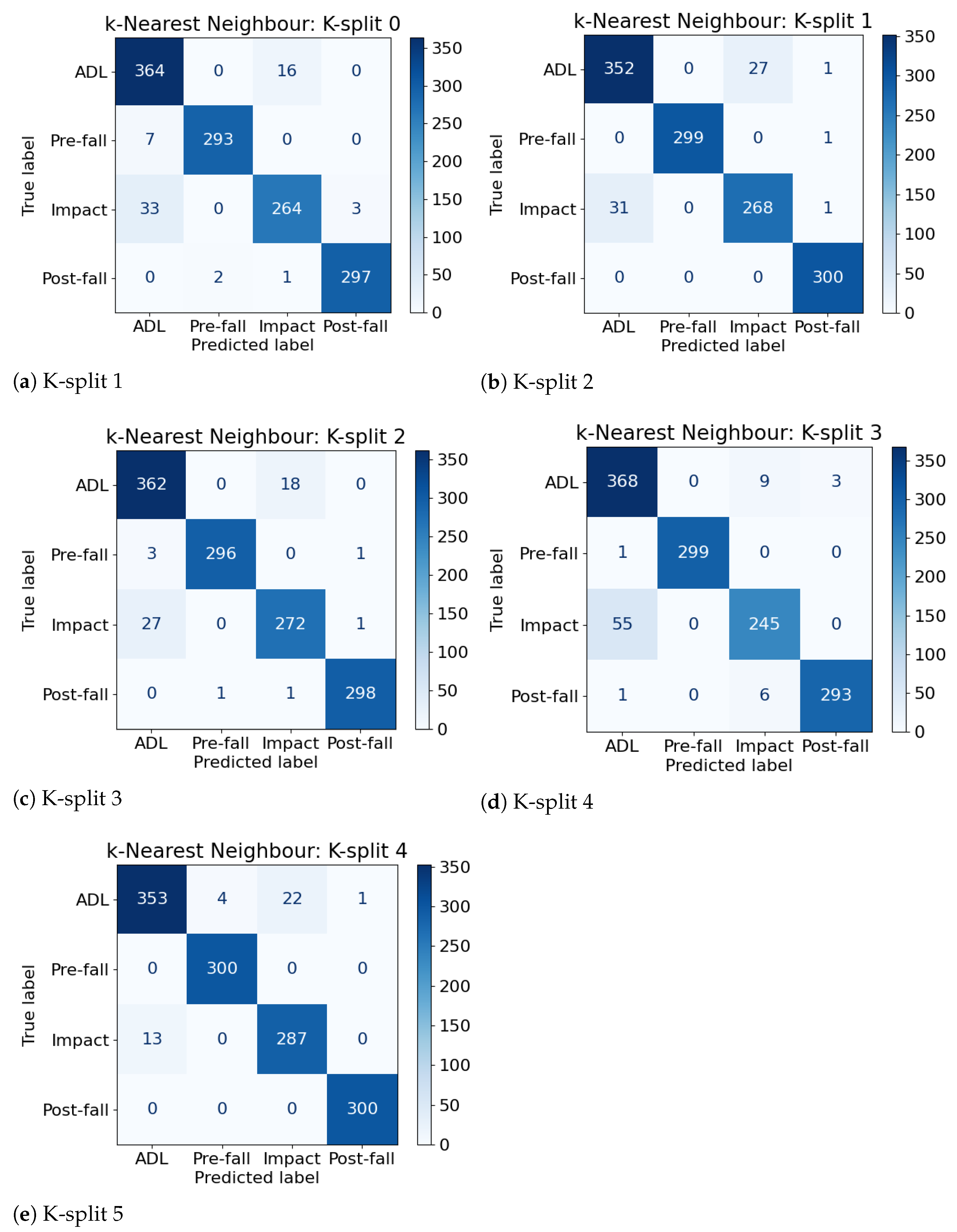
4.3. Multi-Class Approach Performance
5. Conclusions and Future Work
- RQ1
- What is the difference in performance across various types of Machine Learning (ML) algorithms in a FDS?Our FDS implemented several ML algorithms for comparison: k-Nearest Neighbors, Support Vector Machine, Decision Trees, Random Forest and Gradient Boosting. Our results are an improvement over those reported by Musci et al. [36] and Sucerquia et al. [31], with a final Sensitivity and Specificity over 98%. The system is reliable as we were able to test it on a large dataset containing several thousands of Activities of Daily Living (ADLs) and falls. We obtained these results using various ML algorithms which we were able to compare. We observed that ensemble learning algorithms perform better than lazy or eager learning ones. We also further investigated the effect of the sensors’ sampling rate on the detection rate.
- RQ2
- What is the effect of the sensors’ sampling rate on the fall detection?We discovered a tendency that a high sampling rate usually produces better results than a lower one. However, it is not necessary to have an extremely high sampling rate (i.e., in the several hundreds). We recommend using a sampling rate of 50 Hz because it produces improved results with any algorithm while keeping a rather low computational cost.
- RQ3
- What is the difference in performance across various types of ML algorithms by adopting a multi-class approach for identifying phases of a fall?We found that the multi-class approach to identify the phases of a fall showed promising results with an accuracy close to 99%. In addition, it includes key features which are the possibility for improved performance by adding subsequent logic to the ML algorithm to address possible misclassifications. Given this performance, we would advocate this multi-class approach as being useful in a different contexts such as fall prevention systems.
Author Contributions
Funding
Institutional Review Board Statement
Informed Consent Statement
Data Availability Statement
Acknowledgments
Conflicts of Interest
Abbreviations
| ADL | Activity of Daily Living |
| ALS | Assisted-Living System |
| AUROC | Area Under the Receiver Operating Characteristics Curve |
| BDM | Bayesian Decision Making |
| DL | Deep Learning |
| DT | Decision Tree |
| FDS | Fall Detection System |
| FN | False Negative |
| FP | False Positive |
| GB | Gradient Boosting |
| KNN | K-Nearest Neighbor |
| ML | Machine Learning |
| RF | Random Forest |
| SE | Sensitivity |
| SP | Specificity |
| SVM | Support Vector Machine |
| TN | True Negative |
| TP | True Positive |
References
- Rubenstein, L.Z. Falls in older people: Epidemiology, risk factors and strategies for prevention. Age Ageing 2006, 35, ii37–ii41. [Google Scholar] [CrossRef]
- World Health Organization. WHO Global Report on Falls Prevention in Older Age; OCLC: Ocn226291980; World Health Organization: Geneva, Switzerland, 2008. [Google Scholar]
- Sadigh, S.; Reimers, A.; Andersson, R.; Laflamme, L. Falls and Fall-Related Injuries Among the Elderly: A Survey of Residential-Care Facilities in a Swedish Municipality. J. Community Health 2004, 29, 129–140. [Google Scholar] [CrossRef]
- Wild, D.; Nayak, U.S.; Isaacs, B. How dangerous are falls in old people at home? Br. Med. J. (Clin. Res. Ed.) 1981, 282, 266–268. [Google Scholar] [CrossRef] [PubMed]
- Rashidi, P.; Mihailidis, A. A Survey on Ambient-Assisted Living Tools for Older Adults. IEEE J. Biomed. Health Inform. 2013, 17, 579–590. [Google Scholar] [CrossRef] [PubMed]
- Hawley-Hague, H.; Boulton, E.; Hall, A.; Pfeiffer, K.; Todd, C. Older adults’ perceptions of technologies aimed at falls prevention, detection or monitoring: A systematic review. Int. J. Med Inform. 2014, 83, 416–426. [Google Scholar] [CrossRef] [PubMed]
- Noury, N.; Fleury, A.; Rumeau, P.; Bourke, A.K.; Laighin, G.O.; Rialle, V.; Lundy, J.E. Fall detection—Principles and Methods. In Proceedings of the 2007 29th Annual International Conference of the IEEE Engineering in Medicine and Biology Society, Lyon, France, 22–26 August 2007; pp. 1663–1666. [Google Scholar] [CrossRef]
- Zurbuchen, N.; Wilde, A.; Bruegger, P. A Comparison of Machine Learning Algorithms for Fall Detection using Wearable Sensors. In Proceedings of the The 2nd International Conference on Artifical Intelligence in Information and Communication, Fukuoka, Japan, 19–21 February 2020. [Google Scholar]
- Mubashir, M.; Shao, L.; Seed, L. A survey on fall detection: Principles and approaches. Neurocomputing 2013, 100, 144–152. [Google Scholar] [CrossRef]
- Yu, X. Approaches and principles of fall detection for elderly and patient. In Proceedings of the HealthCom 2008—10th International Conference on e-health Networking, Applications and Services, Singapore, 7–9 July 2008; pp. 42–47. [Google Scholar] [CrossRef]
- Abbate, S.; Avvenuti, M.; Bonatesta, F.; Cola, G.; Corsini, P.; Vecchio, A. A smartphone-based fall detection system. Pervasive Mob. Comput. 2012, 8, 883–899. [Google Scholar] [CrossRef]
- Bourke, A.K.; O’Brien, J.V.; Lyons, G.M. Evaluation of a threshold-based tri-axial accelerometer fall detection algorithm. Gait Posture 2007, 26, 194–199. [Google Scholar] [CrossRef]
- Chan, A.M.; Selvaraj, N.; Ferdosi, N.; Narasimhan, R. Wireless patch sensor for remote monitoring of heart rate, respiration, activity, and falls. In Proceedings of the 2013 35th Annual International Conference of the IEEE Engineering in Medicine and Biology Society (EMBC), Osaka, Japan, 3–7 July 2013; pp. 6115–6118. [Google Scholar] [CrossRef]
- Kangas, M.; Konttila, A.; Lindgren, P.; Winblad, I.; Jämsä, T. Comparison of low-complexity fall detection algorithms for body attached accelerometers. Gait Posture 2008, 28, 285–291. [Google Scholar] [CrossRef] [PubMed]
- Yuwono, M.; Moulton, B.D.; Su, S.W.; Celler, B.G.; Nguyen, H.T. Unsupervised machine-learning method for improving the performance of ambulatory fall-detection systems. BioMed. Eng. OnLine 2012, 11, 9. [Google Scholar] [CrossRef]
- Bourke, A.K.; Lyons, G.M. A threshold-based fall-detection algorithm using a bi-axial gyroscope sensor. Med Eng. Phys. 2008, 30, 84–90. [Google Scholar] [CrossRef]
- Tang, M.; Ou, D. Fall Detection System for Monitoring an Elderly Person Based on Six-Axis Gyroscopes. In Proceedings of the 2018 3rd International Conference on Electrical, Automation and Mechanical Engineering (EAME 2018), Xi’an, China, 24–25 June 2018. [Google Scholar] [CrossRef]
- Dinh, A.; Teng, D.; Chen, L.; Shi, Y.; McCrosky, C.; Basran, J.; Bello-Hass, V.D. Implementation of a Physical Activity Monitoring System for the Elderly People with Built-in Vital Sign and Fall Detection. In Proceedings of the 2009 Sixth International Conference on Information Technology: New Generations, Las Vegas, NV, USA, 27–29 April 2009; pp. 1226–1231. [Google Scholar] [CrossRef]
- Wang, J.; Zhang, Z.; Li, B.; Lee, S.; Sherratt, R.S. An enhanced fall detection system for elderly person monitoring using consumer home networks. IEEE Trans. Consum. Electron. 2014, 60, 23–29. [Google Scholar] [CrossRef]
- Fudickar, S.J.; Lindemann, A.; Schnor, B. Threshold-based Fall Detection on Smart Phones. In Proceedings of the HEALTHINF, Angers, France, 3–6 March 2014; pp. 303–309. [Google Scholar] [CrossRef]
- Medrano, C.; Igual, R.; Plaza, I.; Castro, M. Detecting Falls as Novelties in Acceleration Patterns Acquired with Smartphones. PLoS ONE 2014, 9, e94811. [Google Scholar] [CrossRef]
- Hwang, J.Y.; Kang, J.M.; Jang, Y.W.; Kim, H.C. Development of novel algorithm and real-time monitoring ambulatory system using Bluetooth module for fall detection in the elderly. In Proceedings of the The 26th Annual International Conference of the IEEE Engineering in Medicine and Biology Society, San Francisco, CA, USA, 1–5 September 2004; Volume 1, pp. 2204–2207. [Google Scholar] [CrossRef]
- Choi, Y.; Ralhan, A.S.; Ko, S. A Study on Machine Learning Algorithms for Fall Detection and Movement Classification. In Proceedings of the 2011 International Conference on Information Science and Applications, Jeju Island, Korea, 26–29 April 2011; pp. 1–8. [Google Scholar] [CrossRef]
- Gjoreski, H.; Lustrek, M.; Gams, M. Accelerometer Placement for Posture Recognition and Fall Detection. In Proceedings of the 2011 Seventh International Conference on Intelligent Environments, Nottingham, UK, 25–28 July 2011; pp. 47–54. [Google Scholar] [CrossRef]
- Aziz, O.; Robinovitch, S.N. An Analysis of the Accuracy of Wearable Sensors for Classifying the Causes of Falls in Humans. IEEE Trans. Neural Syst. Rehabil. Eng. 2011, 19, 670–676. [Google Scholar] [CrossRef]
- Bagalà, F.; Becker, C.; Cappello, A.; Chiari, L.; Aminian, K.; Hausdorff, J.M.; Zijlstra, W.; Klenk, J. Evaluation of Accelerometer-Based Fall Detection Algorithms on Real-World Falls. PLoS ONE 2012, 7, e37062. [Google Scholar] [CrossRef]
- Özdemir, A.T.; Barshan, B. Detecting Falls with Wearable Sensors Using Machine Learning Techniques. Sensors 2014, 14, 10691–10708. [Google Scholar] [CrossRef]
- Vilarinho, T.; Farshchian, B.; Bajer, D.G.; Dahl, O.H.; Egge, I.; Hegdal, S.S.; Lønes, A.; Slettevold, J.N.; Weggersen, S.M. A Combined Smartphone and Smartwatch Fall Detection System. In Proceedings of the 2015 IEEE International Conference on Computer and Information Technology; Ubiquitous Computing and Communications; Dependable, Autonomic and Secure Computing; Pervasive Intelligence and Computing, Liverpool, UK, 26–28 October 2015; pp. 1443–1448. [Google Scholar] [CrossRef]
- Casilari, E.; Oviedo-Jiménez, M.A. Automatic Fall Detection System Based on the Combined Use of a Smartphone and a Smartwatch. PLoS ONE 2015, 10, e0140929. [Google Scholar] [CrossRef]
- Gibson, R.M.; Amira, A.; Ramzan, N.; Casaseca-de-la Higuera, P.; Pervez, Z. Multiple comparator classifier framework for accelerometer-based fall detection and diagnostic. Appl. Soft Comput. 2016, 39, 94–103. [Google Scholar] [CrossRef]
- Sucerquia, A.; López, J.D.; Vargas-Bonilla, J.F. SisFall: A Fall and Movement Dataset. Sensors 2017, 17, 198. [Google Scholar] [CrossRef]
- Hsieh, C.Y.; Liu, K.C.; Huang, C.N.; Chu, W.C.; Chan, C.T. Novel Hierarchical Fall Detection Algorithm Using a Multiphase Fall Model. Sensors 2017, 17, 307. [Google Scholar] [CrossRef]
- Krupitzer, C.; Sztyler, T.; Edinger, J.; Breitbach, M.; Stuckenschmidt, H.; Becker, C. Hips Do Lie! A Position-Aware Mobile Fall Detection System. In Proceedings of the 2018 IEEE International Conference on Pervasive Computing and Communications (PerCom), Athens, Greece, 19–23 March 2018; pp. 1–10. [Google Scholar] [CrossRef]
- Krupitzer, C.; Sztyler, T.; Edinger, J.; Breitbach, M.; Stuckenschmidt, H.; Becker, C. Beyond position-awareness—Extending a self-adaptive fall detection system. Pervasive Mob. Comput. 2019, 58, 101026. [Google Scholar] [CrossRef]
- Casilari, E.; Lora-Rivera, R.; García-Lagos, F. A Study on the Application of Convolutional Neural Networks to Fall Detection Evaluated with Multiple Public Datasets. Sensors 2020, 20, 1466. [Google Scholar] [CrossRef]
- Musci, M.; De Martini, D.; Blago, N.; Facchinetti, T.; Piastra, M. Online Fall Detection using Recurrent Neural Networks. arXiv 2018, arXiv:1804.04976. [Google Scholar]
- SISTEMIC: SisFall Dataset. 2017. Available online: http://sistemic.udea.edu.co/en/investigacion/proyectos/english-falls/ (accessed on 16 December 2020).
- Nyan, M.N.; Tay, F.E.H.; Murugasu, E. A wearable system for pre-impact fall detection. J. Biomech. 2008, 41, 3475–3481. [Google Scholar] [CrossRef]
- Casilari, E.; Santoyo-Ramón, J.A.; Cano-García, J.M. Analysis of Public Datasets for Wearable Fall Detection Systems. Sensors 2017, 17, 1513. [Google Scholar] [CrossRef]
- Casilari, E.; Santoyo-Ramón, J.A.; Cano-García, J.M. UMAFall: A Multisensor Dataset for the Research on Automatic Fall Detection. Procedia Comput. Sci. 2017, 110, 32–39. [Google Scholar] [CrossRef]
- Micucci, D.; Mobilio, M.; Napoletano, P.; Micucci, D.; Mobilio, M.; Napoletano, P. UniMiB SHAR: A Dataset for Human Activity Recognition Using Acceleration Data from Smartphones. Appl. Sci. 2017, 7, 1101. [Google Scholar] [CrossRef]
- Pedregosa, F.; Varoquaux, G.; Gramfort, A.; Michel, V.; Thirion, B.; Grisel, O.; Blondel, M.; Prettenhofer, P.; Weiss, R.; Dubourg, V.; et al. Scikit-learn: Machine Learning in Python. J. Mach. Learn. Res. 2011, 12, 2825–2830. [Google Scholar]
- Witten, I.H.; Frank, E.; Hall, M.A.; Pal, C.J. Data Mining: Practical Machine Learning Tools and Techniques; Morgan Kaufmann: Burlington, MA, USA, 2017; ISBN 978-0-12-804291-5. [Google Scholar]
- Fawcett, T. An introduction to ROC analysis. Pattern Recognit. Lett. 2006, 27, 861–874. [Google Scholar] [CrossRef]
- Chavarriaga, R.; Sagha, H.; Calatroni, A.; Digumarti, S.T.; Tröster, G.; Millán, J.d.R.; Roggen, D. The Opportunity challenge: A benchmark database for on-body sensor-based activity recognition. Pattern Recognit. Lett. 2013, 34, 2033–2042. [Google Scholar] [CrossRef]
- Ordóñez, F.J.; Roggen, D. Deep Convolutional and LSTM Recurrent Neural Networks for Multimodal Wearable Activity Recognition. Sensors 2016, 16, 115. [Google Scholar] [CrossRef]


| Research Authors (Year) | Sensors | Freq. | Algorithm | Reported Outcomes |
|---|---|---|---|---|
| Hwang et al. [22] (2004) | Accelerometer, gyroscope and tilt sensor placed at the chest. | Not reported | Threshold on each sensor compared sequentially. | Accuracy 96.7% |
| Bourke et al. [12] (2007) | Accelerometer placed at the thigh and chest. | 1 kHz | Double acceleration thresholds applied on both sensors. | SP 100% |
| Bourke et al. [16] (2008) | Bi-axial gyroscope placed at the chest. | 1 kHz | Treble angular thresholds. | SE 100% SP 100% |
| Kangas et al. [14] (2008) | Accelerometer placed at the waist, head and wrist. | 400 Hz | Several simple algorithms including thresholds and posture recognition. | SE 97.5% SP 100% |
| Dinh et al. [18] (2009) | Accelerometer and gyroscope placed at the chest. | 40 Hz | Supervised ML algorithms (SVM, Naïve Bayes, C4.5, Ripple-down rules and RBF. | Accuracy 97% |
| Choi et al. [23] (2011) | Accelerometer and gyroscope placed at the belt. | 10–18 Hz | Naive Bayesian Algorithm to identify specific falls and ADLs. | Accuracy 99.4% |
| Gjoreski et al. [24] (2011) | Four accelerometers placed at the chest, waist, thigh and ankle | 6 Hz | Several simple algorithms including thresholds and posture recognition. | Accuracy 99% |
| Aziz et al. [25] (2011) | Three accelerometers placed at the sternum, right ankle and left ankle | 120 Hz | Linear discriminant analysis to identify three causes of fall. | SE 96% SP 98% |
| Yuwono et al. [15] (2012) | Accelerometer placed at the waist. | 20 Hz | Unsupervised ML algorithms (clustering, MLP and augmented RBF neural network) with WT. | SE 100% SP 99.33% |
| Bagalà et al. [26] (2012) | Accelerometer placed at the lower back. | 100 Hz | Comparison of several threshold-based algorithms with posture recognition. | SE 83% SP 94% |
| Abbate et al. [11] (2012) | Accelerometer from a belt worn smartphone. | 50 Hz | Neural network with 8 features extracted as input and a 4 classes classification. | SE 100% SP 100% |
| Chan et al. [13] (2013) | Three accelerometers placed at the chest. | 62.5 Hz | Combination of thresholds, posture measurements and posture recognition. | SE 95.2% SP 100% |
| Fudickar et al. [20] (2014) | Accelerometer from a smartphone worn at the hip. | 50–800 Hz | Threshold-based with sequential posture recognition. | SE 99% |
| Wang et al. [19] (2014) | Accelerometer and cardiotachometer placed at the chest. | Not reported | Treble thresholds including impact magnitude, trunk angle and heart rate. | SE 96.8% SP 97.5% |
| Medrano et al. [21] (2014) | Smartphone accelerometer in a pocket (for 95% of ADL data), a hand bag (5%), or two smartphones in separate hand bags (for falls). | unstable, 16.7–52 Hz | One-class SVM, kNN (k = 1), kNN-sum (k = 2) and K-means + 1 NN (k = 800) | SE > 89% SP > 88% |
| Özdemir et al. [27] (2014) | Accelerometer, gyroscope and magnetometer placed at the head, chest, back, wrist, ankle and thigh. | 25 Hz | Features extraction at the total peak acceleration and use of ML algorithms (KNN, LSM, SVM, BDM, DTW and ANN). | SE 100% SP > 99% |
| Vilarinho et al. [28] (2015) | Accelerometer and gyroscope from the smartphone and smartwatch respectively placed at the thigh and wrist. | Not reported | Acceleration threshold and pattern recognition from both devices | SE 63% SP 78% |
| Casilari et al. [29] (2015) | Accelerometer and gyroscope from the smartphone and smartwatch respectively placed at the thigh and wrist. | Not reported | Several thresholds compared to each other with every combination of sensors. | SE 96.7% SP 100% |
| Gibson et al. [30] (2016) | Accelerometer placed at the chest. | 50 Hz | Combination of several algorithms (ANN, KNN, RBF, PPCA, LDA) | SE > 90% SP > 90% |
| Sucerquia et al. [31] (2017) | Accelerometer placed at the waist. | 200 Hz | Threshold-based classifier with feature extraction. | Accuracy 96% |
| Hsieh et al. [32] (2017) | Accelerometer placed at the waist. | 128 Hz | Threshold-based Classifier followed by SVM. | Accuracy > 98.74% |
| Krupitzer et al. [33,34] (2018, 2019) | Accelerometers placed at the chest, waist and thigh. | 20–200 Hz | Self-adaptive pervasive fall detection system combining multiple datasets. | SE 75% |
| Tang et al. [17] (2018) | Six-axis gyroscope inside a bracelet worn at the wrist. | Not reported | Three-feature vector fed into SVM. | Accuracy 100% |
| Casilari et al. [35] (2020) | Accelerometry signals from several datasets mainly placed at the waist. | 10–200 Hz | Deep Learning with Convolutional Neural Networks | SE > 98% SP > 98% |
| Characteristics | Casilari et al. [40] (2016) | Sucerquia et al. [31] (2017) | Micucci et al. [41] (2017) |
|---|---|---|---|
| Dataset name | UMAFall | SisFall | UniMiB SHAR |
| No. of sensing points | 5 | 1 | 1 |
| No. of sensors per point | 3 | 3 | 1 |
| Type of sensors | A|G|M | A|A|G | A |
| Positions of the points | Ch|Wa|Wr|Th|An | Wa | Th |
| Sampling rates per sensor [Hz] | 20|20|20|100|20 | 200|200|200 | 50 |
| No. of types of ADL/Falls | 12/3 | 19/15 | 9/8 |
| No. of samples ADL/Falls) | 746 (538/208) | 4505 (2707/1798) | 7013 (5314/1699) |
| No. of subjects (Female/Male) | (8/11) | 38 (19/19) | 30 (24/6) |
| Subjects’ age range | 18–68 | 19–75 | 18–60 |
| Subjects’ weight range [kg] | 50–93 | 41.5–102 | 50–82 |
| Subjects’ height range [cm] | 155–195 | 149–183 | 160–190 |
| Activity | Duration [s] |
|---|---|
| Walking slowly | 100 |
| Walking quickly | 100 |
| Jogging slowly | 100 |
| Jogging quickly | 100 |
| Walking upstairs and downstairs slowly | 25 |
| Walking upstairs and downstairs quickly | 25 |
| Slowly sit and get up in a half-height chair | 12 |
| Quickly sit and get up in a half-height chair | 12 |
| Slowly sit and get up in a low-height chair | 12 |
| Quickly sit and get up in a low-height chair | 12 |
| Sitting, trying to get up, and collapse into a chair | 12 |
| Sitting, lying slowly, wait a moment, and sit again | 12 |
| Sitting, lying quickly, wait a moment, and sit again | 12 |
| Changing position while lying (back-lateral-back) | 12 |
| Standing, slowly bending at knees, and getting up | 12 |
| Standing, slowly bending w/o knees, and getting up | 12 |
| Standing, get into and get out of a car | 25 |
| Stumble while walking | 12 |
| Gently jump without falling (to reach a high object) | 12 |
| Fall forward while walking, caused by a slip | 15 |
| Fall backward while walking, caused by a slip | 15 |
| Lateral fall while walking, caused by a slip | 15 |
| Fall forward while walking, caused by a trip | 15 |
| Fall forward while jogging, caused by a trip | 15 |
| Vertical fall while walking, caused by fainting | 15 |
| Fall while walking with damping, caused by fainting | 15 |
| Fall forward when trying to get up | 15 |
| Lateral fall when trying to get up | 15 |
| Fall forward when trying to sit down | 15 |
| Fall backward when trying to sit down | 15 |
| Lateral fall when trying to sit down | 15 |
| Fall forward while sitting, caused by fainting | 15 |
| Fall backward while sitting, caused by fainting | 15 |
| Lateral fall while sitting, caused by fainting | 15 |
| Feature Classes | Domain |
|---|---|
| Variance | Time |
| Standard deviation | Time |
| Mean | Time |
| Median | Time |
| Maximum | Time |
| Minimum | Time |
| Delta (peak-to-peak) | Time |
| 25th Centile | Time |
| 75th Centile | Time |
| Power Spectral Density | Frequency |
| Power Spectral Entropy | Frequency |
| Frequency [Hz] | KNN [%] | SVM [%] | DT [%] | RF [%] | GB [%] |
|---|---|---|---|---|---|
| 1 | 85.66 | 74.13 | 91.26 | 93.60 | 95.33 |
| 2 | 91.46 | 77.93 | 91.33 | 95.53 | 96.86 |
| 5 | 95.33 | 84.86 | 94.73 | 95.66 | 98.06 |
| 10 | 96.53 | 88.80 | 94.73 | 97.26 | 98.40 |
| 20 | 97.20 | 91.80 | 95.80 | 97.66 | 98.26 |
| 50 | 97.40 | 91.80 | 96.26 | 98.20 | 98.13 |
| 100 | 97.40 | 93.89 | 96.40 | 97.73 | 98.20 |
| 200 | 97.26 | 93.78 | 96.60 | 98.00 | 98.06 |
| Frequency [Hz] | KNN [%] | SVM [%] | DT [%] | RF [%] | GB [%] |
|---|---|---|---|---|---|
| 1 | 94.68 | 80.21 | 93.00 | 96.21 | 96.21 |
| 2 | 97.05 | 83.73 | 94.26 | 97.42 | 97.57 |
| 5 | 98.78 | 88.68 | 96.32 | 98.68 | 98.47 |
| 10 | 99.57 | 90.89 | 96.73 | 99.42 | 98.47 |
| 20 | 99.68 | 92.15 | 97.52 | 99.21 | 99.10 |
| 50 | 99.42 | 93.26 | 96.63 | 99.15 | 98.73 |
| 100 | 99.42 | 93.89 | 97.26 | 99.15 | 98.94 |
| 200 | 99.31 | 93.78 | 97.26 | 98.94 | 99.21 |
| Frequency [Hz] | KNN [%] | SVM [%] | DT [%] | RF [%] | GB [%] |
|---|---|---|---|---|---|
| 1 | 90.70 | 77.52 | 92.23 | 95.05 | 95.82 |
| 2 | 94.58 | 81.17 | 92.97 | 96.58 | 97.26 |
| 5 | 97.26 | 87.00 | 95.61 | 97.35 | 98.29 |
| 10 | 98.23 | 89.97 | 95.85 | 98.47 | 98.44 |
| 20 | 98.58 | 92.00 | 96.76 | 98.52 | 98.73 |
| 50 | 98.52 | 92.61 | 96.47 | 98.73 | 98.47 |
| 100 | 98.52 | 92.05 | 96.88 | 98.52 | 98.61 |
| 200 | 98.41 | 91.20 | 96.97 | 98.52 | 98.70 |
| Frequency [Hz] | KNN [%] | SVM [%] | DT [%] | RF [%] | GB [%] |
|---|---|---|---|---|---|
| 1 | 88.98 | 74.35 | 91.18 | 94.28 | 95.24 |
| 2 | 93.68 | 78.47 | 91.97 | 96.08 | 96.88 |
| 5 | 96.81 | 85.17 | 94.99 | 96.94 | 98.06 |
| 10 | 97.93 | 88.56 | 95.25 | 98.23 | 98.23 |
| 20 | 98.36 | 90.93 | 96.29 | 98.30 | 98.55 |
| 50 | 98.30 | 91.55 | 95.99 | 98.55 | 98.25 |
| 100 | 98.30 | 90.76 | 96.45 | 98.31 | 98.42 |
| 200 | 98.17 | 89.70 | 96.55 | 98.31 | 98.52 |
| Frequency [Hz] | KNN [%] | SVM [%] | DT [%] | RF [%] | GB [%] |
|---|---|---|---|---|---|
| 1 | 95.97 | 86.02 | 92.13 | 98.72 | 99.12 |
| 2 | 97.73 | 90.17 | 92.79 | 99.26 | 99.61 |
| 5 | 99.03 | 93.83 | 95.52 | 99.60 | 99.87 |
| 10 | 99.49 | 96.14 | 95.73 | 99.85 | 99.93 |
| 20 | 99.50 | 97.35 | 96.66 | 99.85 | 99.92 |
| 50 | 99.44 | 97.66 | 96.44 | 99.87 | 99.93 |
| 100 | 99.36 | 97.13 | 96.83 | 99.86 | 99.93 |
| 200 | 99.45 | 96.43 | 96.93 | 99.90 | 99.93 |
Publisher’s Note: MDPI stays neutral with regard to jurisdictional claims in published maps and institutional affiliations. |
© 2021 by the authors. Licensee MDPI, Basel, Switzerland. This article is an open access article distributed under the terms and conditions of the Creative Commons Attribution (CC BY) license (http://creativecommons.org/licenses/by/4.0/).
Share and Cite
Zurbuchen, N.; Wilde, A.; Bruegger, P. A Machine Learning Multi-Class Approach for Fall Detection Systems Based on Wearable Sensors with a Study on Sampling Rates Selection. Sensors 2021, 21, 938. https://doi.org/10.3390/s21030938
Zurbuchen N, Wilde A, Bruegger P. A Machine Learning Multi-Class Approach for Fall Detection Systems Based on Wearable Sensors with a Study on Sampling Rates Selection. Sensors. 2021; 21(3):938. https://doi.org/10.3390/s21030938
Chicago/Turabian StyleZurbuchen, Nicolas, Adriana Wilde, and Pascal Bruegger. 2021. "A Machine Learning Multi-Class Approach for Fall Detection Systems Based on Wearable Sensors with a Study on Sampling Rates Selection" Sensors 21, no. 3: 938. https://doi.org/10.3390/s21030938
APA StyleZurbuchen, N., Wilde, A., & Bruegger, P. (2021). A Machine Learning Multi-Class Approach for Fall Detection Systems Based on Wearable Sensors with a Study on Sampling Rates Selection. Sensors, 21(3), 938. https://doi.org/10.3390/s21030938