Detecting and Tracking the Positions of Wild Ungulates Using Sound Recordings

 ,
, 
Abstract
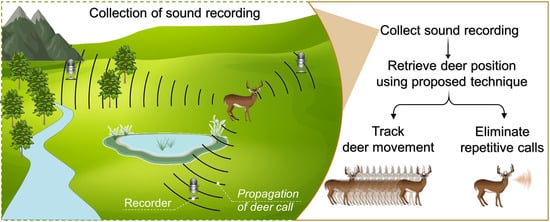
1. Introduction
2. Methods
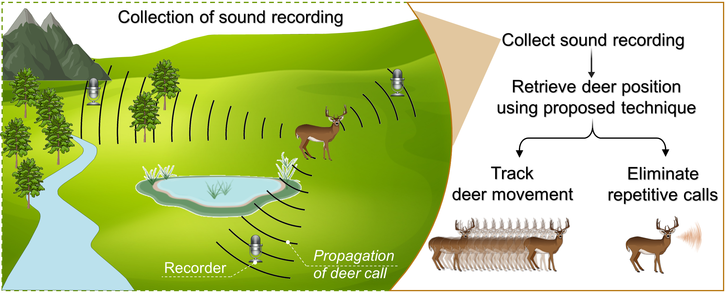
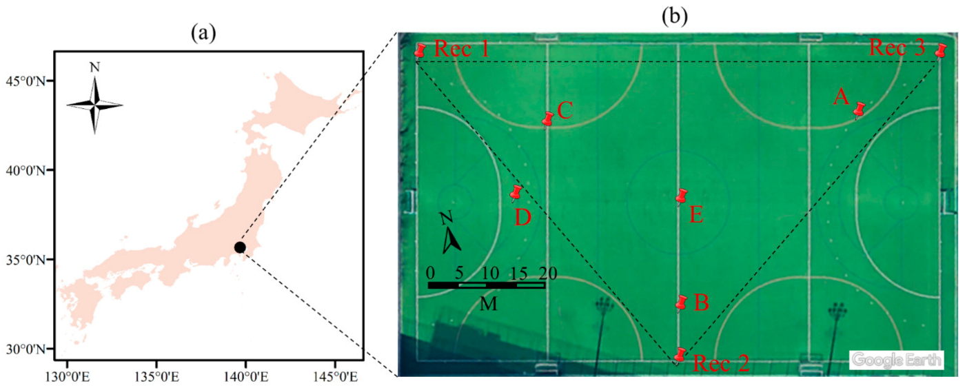
2.1. Study Area
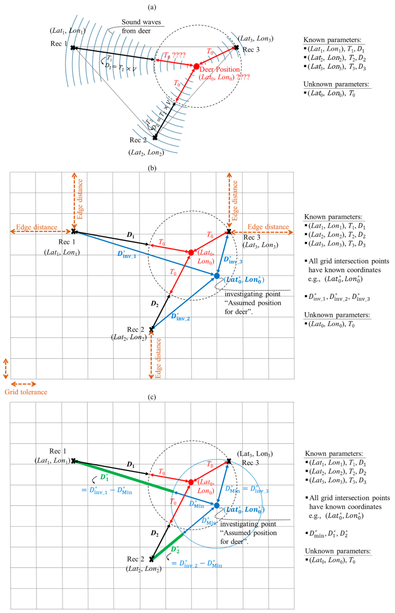
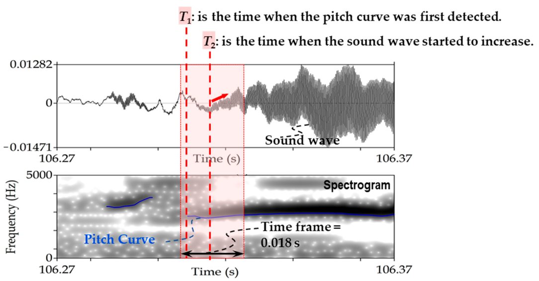
2.2. Description of Proposed Technique
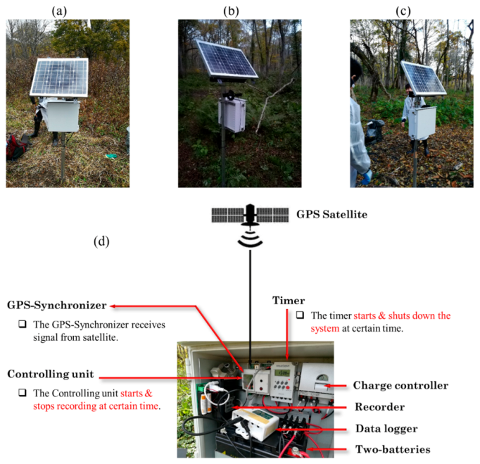
2.3. Development of Sound Recording System
2.4. Distance between Sound Recording Units
3. Results and Discussion
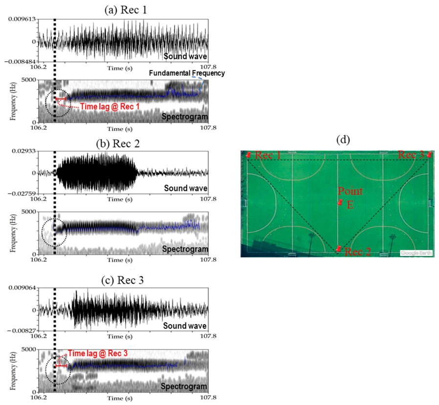
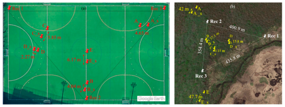
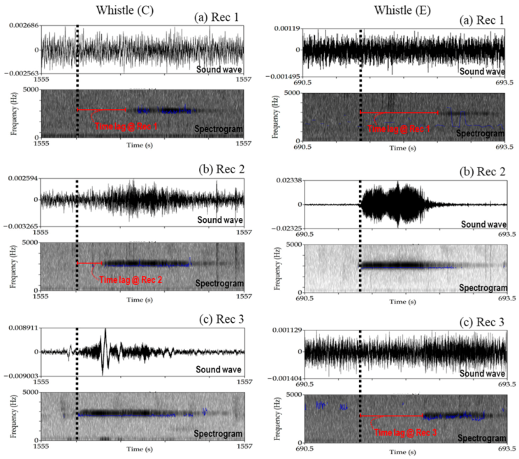
3.1. Validation of the UTokyo Experiment
3.2. Validation of the Oze Marshland Experiment
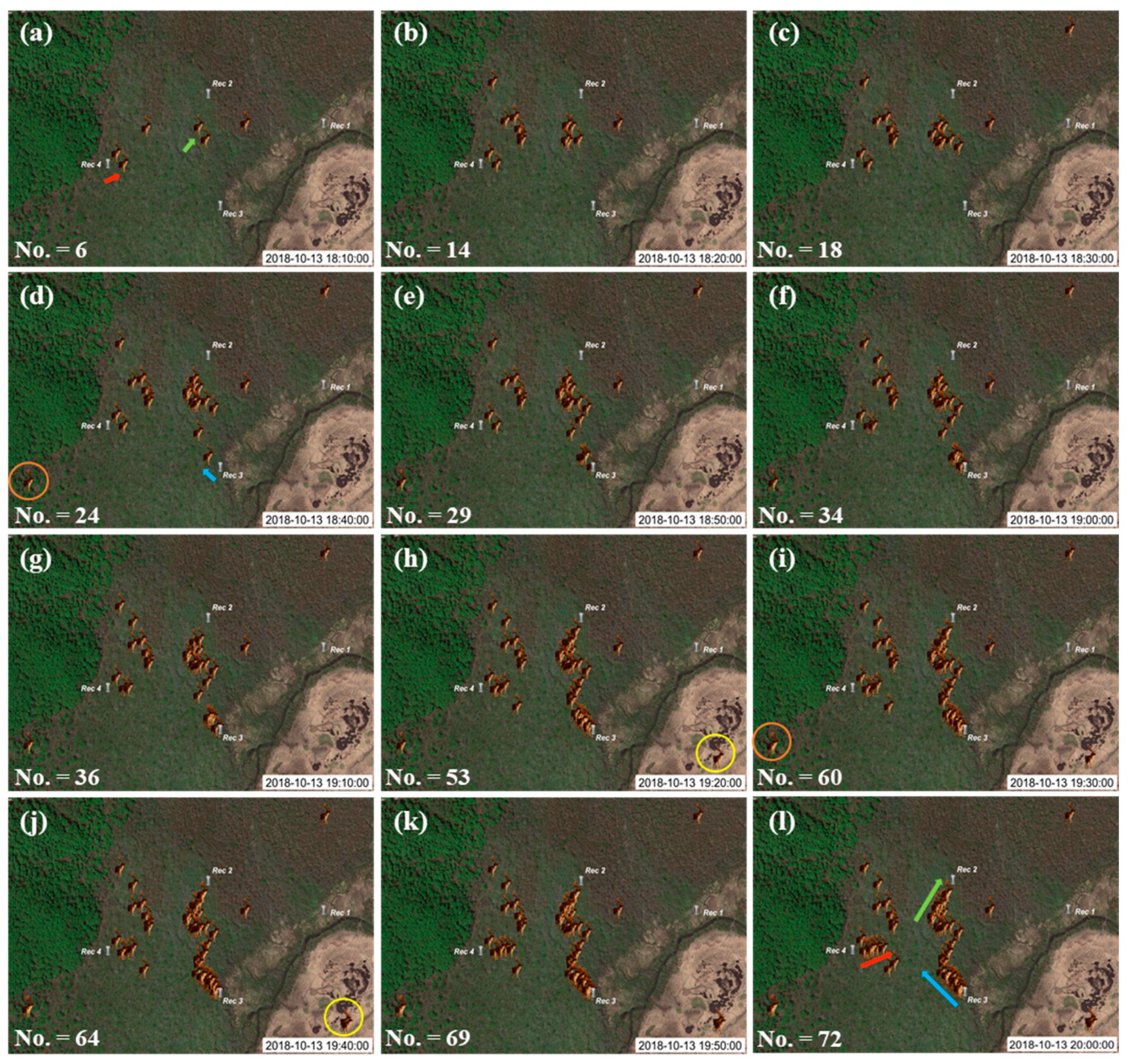
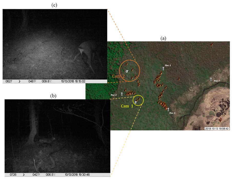
3.3. Tracking Deer Calls in Oze
4. Conclusions and Recommendations
Supplementary Materials
Author Contributions
Funding
Institutional Review Board Statement
Informed Consent Statement
Acknowledgments
Conflicts of Interest
References
- Acevedo, P.; Ruiz-Fons, F.; Vicente, J.; Reyes-García, A.R.; Alzaga, V.; Gortázar, C. Estimating red deer abundance in a wide range of management situations in Mediterranean habitats. J. Zool. 2008, 276, 37–47. [Google Scholar] [CrossRef]
- Enari, H.; Enari, H.; Okuda, K.; Yoshita, M.; Kuno, T.; Okuda, K. Feasibility assessment of active and passive acoustic monitoring of sika deer populations. Ecol. Indic. 2017, 79, 155–162. [Google Scholar] [CrossRef]
- Ando, M.; Shibata, E. Bark-Stripping Preference of Sika Deer and Its Seasonality on Mt. Ohdaigahara, Central Japan. In Sika Deer; Springer: Berlin/Heidelberg, Germany, 2009; pp. 207–216. [Google Scholar]
- Morellet, N.; Gaillard, J.; Hewison, A.J.M.; Ballon, P.; Boscardin, Y.; Duncan, P.; Klein, F.; Maillard, D. Indicators of ecological change: New tools for managing populations of large herbivores. J. Appl. Ecol. 2007, 44, 634–643. [Google Scholar] [CrossRef]
- Naito, T.; Kimura, Y. Sika deer in the Oze area. In A Comprehensive Study of the Oze Area; Oze Research Group: Maebashi, Japan, 1998; pp. 725–739. [Google Scholar]
- Takafumi, H.; Kamii, T.; Murai, T.; Yoshida, R.; Sato, A.; Tachiki, Y.; Akamatsu, R.; Yoshida, T. Seasonal and year-round use of the Kushiro Wetland, Hokkaido, Japan by sika deer (Cervus nippon yesoensis). PeerJ 2017, 5, e3869. [Google Scholar] [CrossRef] [PubMed]
- Takatsuki, S. Effects of sika deer on vegetation in Japan: A review. Biol. Conserv. 2009, 142, 1922–1929. [Google Scholar] [CrossRef]
- Enari, H.; Enari, H.S.; Okuda, K.; Maruyama, T.; Okuda, K.N. An evaluation of the efficiency of passive acoustic monitoring in detecting deer and primates in comparison with camera traps. Ecol. Indic. 2019, 98, 753–762. [Google Scholar] [CrossRef]
- Takayama, K.; Sonoda, A.; Hayashida, Y.; Ishii, D.; Yanagita, D.; Matsumoto, S.; Katahira, K.; Oshima, I.; Nakanishi, Y.; Inaome, T.; et al. Wild Sika Deer Invasions of the Grasslands within Livestock Farms. J. Warm Reg. Soc. Anim. Sci. 2017, 60, 21–26. [Google Scholar]
- Clare, J.; McKinney, S.T.; DePue, J.E.; Loftin, C.S. Pairing field methods to improve inference in wildlife surveys while accommodating detection covariance. Ecol. Appl. 2017, 27, 2031–2047. [Google Scholar] [CrossRef]
- Nakano, T.; Bavuudorj, G.; Iijima, Y.; Ito, T.Y. Quantitative evaluation of grazing effect on nomadically grazed grassland ecosystems by using time-lapse cameras. Agric. Ecosyst. Environ. 2020, 287, 106685. [Google Scholar] [CrossRef]
- Nakashima, Y.; Hongo, S.; Akomo-Okoue, E.F. Landscape-scale estimation of forest ungulate density and biomass using camera traps: Applying the REST model. Biol. Conserv. 2020, 241, 108381. [Google Scholar] [CrossRef]
- Lahkar, D.; Ahmed, M.F.; Begum, R.H.; Das, S.K.; Harihar, A. Responses of a wild ungulate assemblage to anthropogenic influences in Manas National Park, India. Biol. Conserv. 2020, 243, 108425. [Google Scholar] [CrossRef]
- Igarashi, T.; Takatsuki, S. Effects of defoliation and digging caused by sika deer on the Oze mires of central Japan. Biosph. Conserv. Nat. Wildl. Hum. 2008, 9, 9–16. [Google Scholar]
- Abdalla, M.; Hastings, A.; Chadwick, D.R.; Jones, D.L.; Evans, C.D.; Jones, M.B.; Rees, R.M.; Smith, P. Critical review of the impacts of grazing intensity on soil organic carbon storage and other soil quality indicators in extensively managed grasslands. Agric. Ecosyst. Environ. 2018, 253, 62–81. [Google Scholar] [CrossRef] [PubMed]
- Steen, K.A.; Villa-Henriksen, A.; Therkildsen, O.R.; Green, O. Automatic detection of animals in mowing operations using thermal cameras. Sensors 2012, 12, 7587–7597. [Google Scholar] [CrossRef] [PubMed]
- Alves, J.; da Silva, A.A.; Soares, A.M.V.M.; Fonseca, C. Pellet group count methods to estimate red deer densities: Precision, potential accuracy and efficiency. Mamm. Biol. 2013, 78, 134–141. [Google Scholar] [CrossRef]
- Kimuyu, D.M.; Veblen, K.E.; Riginos, C.; Chira, R.M.; Githaiga, J.M.; Young, T.P. Influence of cattle on browsing and grazing wildlife varies with rainfall and presence of megaherbivores. Ecol. Appl. 2017, 27, 786–798. [Google Scholar] [CrossRef]
- Kufeld, R.C.; Olterman, J.H.; Bowden, D.C. A helicopter quadrat census for mule deer on Uncompahgre Plateau, Colorado. J. Wildl. Manag. 1980, 632–639. [Google Scholar] [CrossRef]
- Krebs, C.J. Ecological Methodology; Harper & Row: New York, NY, USA, 1989. [Google Scholar]
- Poulsen, J.R.; Clark, C.J.; Bolker, B.M. Decoupling the effects of logging and hunting on an Afrotropical animal community. Ecol. Appl. 2011, 21, 1819–1836. [Google Scholar] [CrossRef]
- Walsh, P.D.; White, L.J.T. Evaluating the steady state assumption: Simulations of gorilla nest decay. Ecol. Appl. 2005, 15, 1342–1350. [Google Scholar] [CrossRef]
- Mourão, G.; Coutinho, M.; Mauro, R.; Campos, Z.; Tomás, W.; Magnusson, W. Aerial surveys of caiman, marsh deer and pampas deer in the Pantanal Wetland of Brazil. Biol. Conserv. 2000, 92, 175–183. [Google Scholar] [CrossRef]
- Hodgson, J.C.; Baylis, S.M.; Mott, R.; Herrod, A.; Clarke, R.H. Precision wildlife monitoring using unmanned aerial vehicles. Sci. Rep. 2016, 6, 22574. [Google Scholar] [CrossRef] [PubMed]
- Wang, D.; Shao, Q.; Yue, H. Surveying Wild Animals from Satellites, Manned Aircraft and Unmanned Aerial Systems (UASs): A Review. Remote Sens. 2019, 11, 1308. [Google Scholar] [CrossRef]
- Barbedo, J.G.A.; Koenigkan, L.V.; Santos, T.T.; Santos, P.M. A Study on the Detection of Cattle in UAV Images Using Deep Learning. Sensors 2019, 19, 5436. [Google Scholar] [CrossRef] [PubMed]
- Drake, K.L.; Frey, M.; Hogan, D.; Hedley, R. Using digital recordings and sonogram analysis to obtain counts of yellow rails. Wildl. Soc. Bull. 2016, 40, 346–354. [Google Scholar] [CrossRef]
- Aihara, I.; Bishop, P.J.; Ohmer, M.E.B.; Awano, H.; Mizumoto, T.; Okuno, H.G.; Narins, P.M.; Hero, J.-M. Visualizing phonotactic behavior of female frogs in darkness. Sci. Rep. 2017, 7, 10539. [Google Scholar] [CrossRef]
- Kessel, S.T.; Cooke, S.J.; Heupel, M.R.; Hussey, N.E.; Simpfendorfer, C.A.; Vagle, S.; Fisk, A.T. A review of detection range testing in aquatic passive acoustic telemetry studies. Rev. Fish Biol. Fish. 2014, 24, 199–218. [Google Scholar] [CrossRef]
- Marques, T.A.; Thomas, L.; Martin, S.W.; Mellinger, D.K.; Ward, J.A.; Moretti, D.J.; Harris, D.; Tyack, P.L. Estimating animal population density using passive acoustics. Biol. Rev. 2013, 88, 287–309. [Google Scholar] [CrossRef]
- Minami, M. Vocal Repertoire and the Functions of Vocalization in the Rutting Season in Sika Deer, Cervus Nippon; Osaka City University: Osaka, Japan, 1997. [Google Scholar]
- Tayanin, D.; Lindell, K. Hunting and Fishing in a Kammu Village: Revisiting a Classic Study in Southeast Asian Ethnography; NIAS Press: Copenhagen, Denmark, 2012. [Google Scholar]
- Ninan, K.N.; Inoue, M. Valuing forest ecosystem services: Case study of a forest reserve in Japan. Ecosyst. Serv. 2013, 5, 78–87. [Google Scholar] [CrossRef]
- Goto, T. Wildlife Management Office (WMO) Field Note No.141. Available online: http://wmo.co.jp/field_note/no-141 (accessed on 1 February 2020).
- NLNI Lakes Data, National Land Numerical Information, Japan. Available online: http://nlftp.mlit.go.jp/ksj/ (accessed on 14 March 2017).
- Veness, C. Calculate Distance and Bearing between Two Latitude/Longitude Points. Available online: https://www.movable-type.co.uk/scripts/latlong.html (accessed on 10 April 2018).
- Chai, T.; Draxler, R.R. Root mean square error (RMSE) or mean absolute error (MAE)?—Arguments against Avoiding RMSE in the Literature. Geosci. Model Dev. 2014, 7, 1247–1250. [Google Scholar] [CrossRef]
- Kamei, T.; Takeda, K.; Izumiyama, S.; Ohshima, K. The effect of hunting on the behavior and habitat utilization of sika deer (Cervus nippon). Mammal Study 2010, 35, 235–241. [Google Scholar] [CrossRef]
- Boersma, P. Praat, a system for doing phonetics by computer. Glot Int. 2001, 2, 341–347. [Google Scholar]
- Audacity. Audacity (R): Free Audio Editor and Recorder, Version 2.0.6. Available online: http://windinthew.users.sourceforge.net/?lang=en (accessed on 26 January 2021).
- Lavi; Ahuja, A.K. Speech Signal De-noising using Wavelet Transform and Different Standard Softwares: Performance Evaluation and Comparisons Study. In Proceedings of the 2018 5th IEEE Uttar Pradesh Section International Conference on Electrical, Electronics and Computer Engineering (UPCON), Gorakhpur, India, 2–4 November 2018; pp. 1–6. [Google Scholar]
- Castro, I.; De Rosa, A.; Priyadarshani, N.; Bradbury, L.; Marsland, S. Experimental test of birdcall detection by autonomous recorder units and by human observers using broadcast. Ecol. Evol. 2019, 9, 2376–2397. [Google Scholar] [CrossRef] [PubMed]
- Priyadarshani, N.; Castro, I.; Marsland, S. The impact of environmental factors in birdsong acquisition using automated recorders. Ecol. Evol. 2018, 8, 5016–5033. [Google Scholar] [CrossRef] [PubMed]


| UTokyo Experiment Site | Oze National Park | ||||
|---|---|---|---|---|---|
| Lat | Long | Lat | Long | ||
| Rec1 | 35°39′38.12″ N | 139°40′54.13″ E | Rec1 | 36°56′31.91″ N | 139°13′38.43″ E |
| Rec2 | 35°39′36.19″ N | 139°40′55.57″ E | Rec2 | 36°56′34.92″ N | 139°13′22.63″ E |
| Rec3 | 35°39′37.63″ N | 139°40′57.72″ E | Rec3 | 36°56′23.49″ N | 139°13′24.27″ E |
| A | 35°39′37.38″ N | 139°40′57.09″ E | Rec4 | 36°56′27.78″ N | 139°13′08.86″ E |
| B | 35°39′36.48″ N | 139°40′55.63″ E | A | 36°56′38.62″ N | 139°13′18.70″ E |
| C | 35°39′37.61″ N | 139°40′54.96″ E | B | 36°56′30.14″ N | 139°13′23.51″ E |
| D | 35°39′37.23″ N | 139°40′54.66″ E | C | 36°56′28.36″ N | 139°13′25.95″ E |
| E | 35°39′37.06″ N | 139°40′55.76″ E | D | 36°56′30.29″ N | 139°13′29.18″ E |
| E | 36°56′19.48″ N | 139°13′25.56″ E | |||
| Distance from Rec 1 | 181 m | 297 m | 423 m | 545 m | 761 m |
|---|---|---|---|---|---|
| Audibility of sound | O | O | O | X |
Publisher’s Note: MDPI stays neutral with regard to jurisdictional claims in published maps and institutional affiliations. |
© 2021 by the authors. Licensee MDPI, Basel, Switzerland. This article is an open access article distributed under the terms and conditions of the Creative Commons Attribution (CC BY) license (http://creativecommons.org/licenses/by/4.0/).
Share and Cite
Salem, S.I.; Fujisao, K.; Maki, M.; Okumura, T.; Oki, K. Detecting and Tracking the Positions of Wild Ungulates Using Sound Recordings. Sensors 2021, 21, 866. https://doi.org/10.3390/s21030866
Salem SI, Fujisao K, Maki M, Okumura T, Oki K. Detecting and Tracking the Positions of Wild Ungulates Using Sound Recordings. Sensors. 2021; 21(3):866. https://doi.org/10.3390/s21030866
Chicago/Turabian StyleSalem, Salem Ibrahim, Kazuhiko Fujisao, Masayasu Maki, Tadanobu Okumura, and Kazuo Oki. 2021. "Detecting and Tracking the Positions of Wild Ungulates Using Sound Recordings" Sensors 21, no. 3: 866. https://doi.org/10.3390/s21030866
APA StyleSalem, S. I., Fujisao, K., Maki, M., Okumura, T., & Oki, K. (2021). Detecting and Tracking the Positions of Wild Ungulates Using Sound Recordings. Sensors, 21(3), 866. https://doi.org/10.3390/s21030866