Abstract
This paper presents a systematization and a comparison of the binary successive approximation (SA) variants. Three different variants are distinguished and all of them are applied in the analog-to-digital conversion. Regardless of an analog-to-digital converter circuit solution, the adoption of the specific SA variant imposes a particular character of the conversion process and related parameters. One of them is the ability to direct conversion of non-removeable physical quantities such as time intervals. Referencing to this aspect a general systematization of the variants and a name for each of them is proposed. In addition, the article raises the issues related to the complexity of implementation and energy consumption for each of the discussed binary SA variants.
1. Introduction
The successive approximation (SA) method is known at least from the 16th century [1]. One of its most common applications was conversion weight of an object to numbers, which in fact is simple analog-to-digital conversion already.
The first implementation of the binary SA scheme in electronic analog-to-digital conversion dates back to the 1950s. Developed for decades it has become fundamental and one of the most successful analog-to-digital conversion techniques. Nowadays, it is usually chosen as compromise between fast but expensive flash and precise but slow integrating analog-to-digital conversion method [1,2,3].
From the very first SA analog-to-digital converter (ADC) all of the solutions based on one of the three binary SA variants. However, in most cases the clear statement referencing to applied SA variant is omitted. Moreover, in literature the SA method itself is often incorrectly identified with only one SA variant. This is possibly caused by a lack of systematization. Therefore, based on the most distinctive parameters of the binary SA variants, a name for each of them is proposed.
Each of the three SA variants has specific properties and one of them is the ability to direct conversion of some non-removable physical quantities such as time intervals. There are cases, where it plays a crucial role and its lack can be an inconvenient obstacle or even disqualifying limitation [4]. If only for this reason, the awareness of differences between the SA variants is important, because it allows to choose the most appropriate one for a specific application.
The following sections are focused especially on the systematization and naming of the SA variants based on the above-mentioned ability to direct conversion of some physical quantities. In addition, the issues of energy consumption and complexity of implementation are discussed.
2. The Binary Successive Approximation Variants
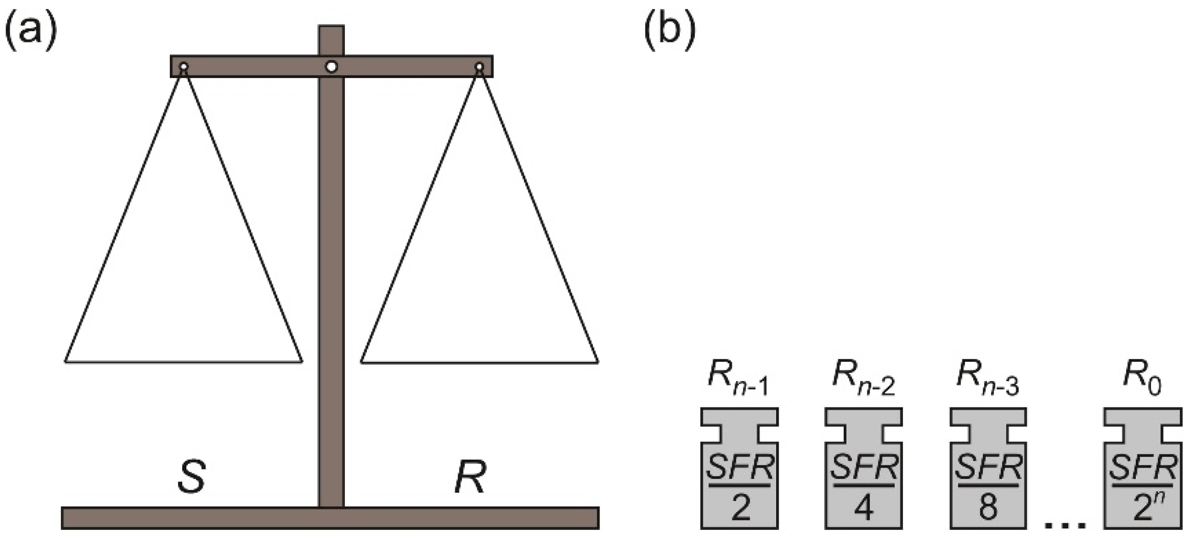
In general, the binary SA method approximates the measured input value XIN with an appropriate subset of predefined, binary-scaled reference units. The unique character of the SA is derived from a very well-known weighing method, which uses a pan balance and a set of reference elements. This is one of the reasons why it is convenient to illustrate the binary SA method as a weighing process. Such an approach is also used in the following analysis in order to explain the differences between the presented algorithms. Both the pan balance and the reference elements are shown in Figure 1.

Figure 1.
The model of the binary SA conversion system: (a) the pan balance model; (b) the binary-scaled reference elements.
The used model of the balance consists of the source pan S and the reference pan R (Figure 1a). The binary-scaled reference elements Rn−1, …, R0 (Figure 1b) are placed on the pans in order to accomplish appropriate binary SA algorithm. The measured input value XIN is always placed on the pan S, but the placement of the reference elements Rn−1, …, R0 depends on the applied SA variant.
The values of the reference elements Rn−1, …, R0 are defined as Rk = 2kR0, for k = 0, 1, …, n − 1. Obviously, there is an accurate relation between the reference elements Rn−1, …, R0 and the parameters of the pan weighing. First of all, with n reference elements Rn−1, …, R0 it is possible to represent the measured input value XIN as one of the 2n different subsets of the reference elements Rn−1, …, R0. Moreover, the total weight of the subsets can vary in range ⟨0, R0, …, (2n − 1)R0⟩. Secondly, because of the finite number of the reference elements Rn−1, …, R0, the resolution of the conversion process is also finite.
Considering the above, the input weight XIN is always measured with determined resolution R0. In addition, it has to be less than 2nR0 in order to be properly measured. This limiting value can be termed as signal full range (SFR):
2.1. Oscillating Successive Approximation
The first variant of the binary SA method requires one set of the reference elements Rn−1, …, R0. Their placement is limited to the pan R only.
The conversion process starts from placing the measured input element XIN on the pan S. Simultaneously, the biggest reference element Rn−1 is placed on the pan R (Figure 2a). At each next step, until the smallest reference element R0 is used, two operations are performed. Firstly, the current state of the pan balance is analyzed. If the total weight of the reference elements currently placed on the pan R is not greater than the weight of the measured input value XIN (Figure 2a), the most recently placed reference element Rk is left on the pan R. Otherwise, the most recently placed reference element Rk is removed from the pan R (Figure 2b,c), which means a change of the previously made decision. Secondly, in both cases, twice smaller reference element Rk−1 (k ≥ 1) is placed on the pan R.
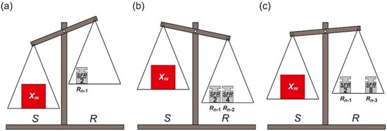
Figure 2.
Illustration of oscillating successive approximation steps: (a) the first step; (b) the overestimation; (c) compensation of the overestimation.
The last step of the conversion process is made after the placement of the smallest reference element R0 on the pan R. It is limited only to decision if the reference element R0 should be removed from the pan R or not.
When the conversion process is completed the measured input value XIN is approximated by an appropriate subset of the reference elements which are left on the pan R. Thus, the final result of the conversion process can be expressed as:
where Pk indicates if the k-th reference element Rk has been left on the pan R (Pk = 1) or not (Pk = 0).
Figure 3 presents the conversion process in the time domain. Performed operations of adding and optional removing the reference elements Rn−1, …, R0 from the pan R cause oscillations around the measured input value XIN. Therefore, the name oscillating successive approximation (OSA) is proposed for this algorithm [5].
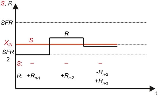
Figure 3.
Oscillating successive approximation process in the time domain.
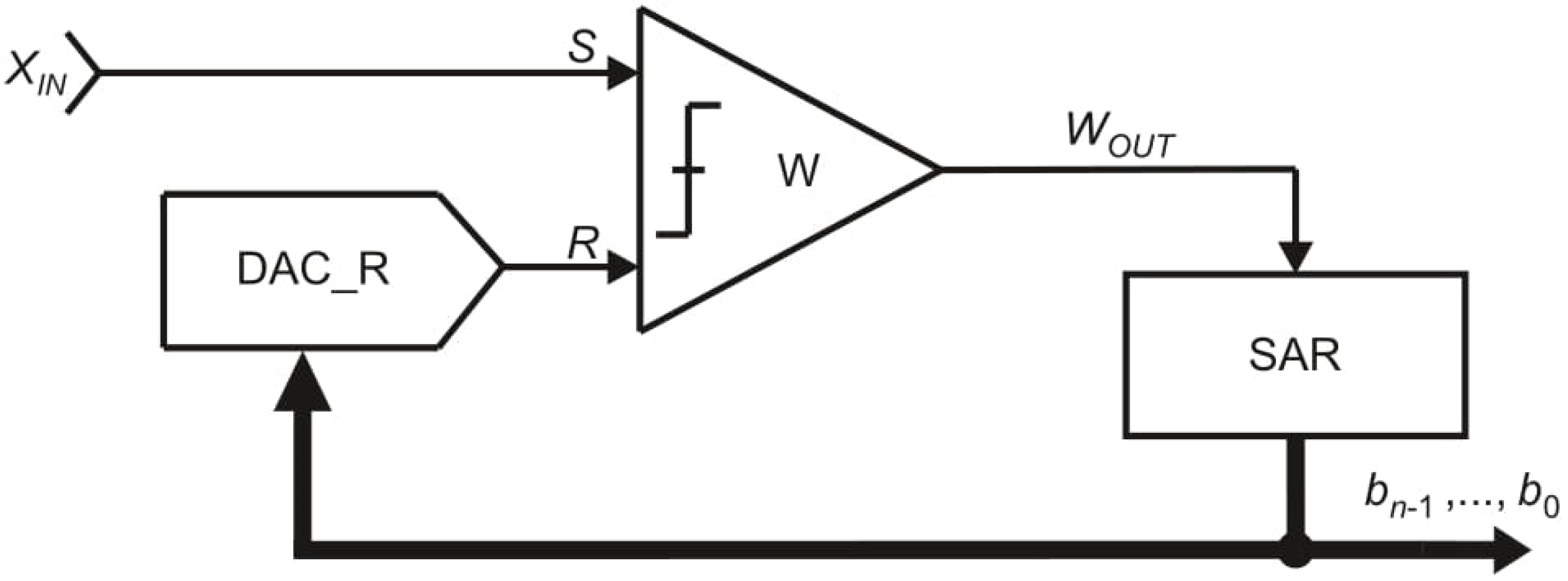
The model of the OSA converter is shown in Figure 4. It consists of one comparator W, one digital-to-analog converter DAC_R and a control logic block SAR (Successive Approximation Register). The inputs of the comparator W, signed as S and R, refer accordingly to the pans S and R. The digital-to-analog converter DAC_R in reference path generates the reference signal R. The comparator W compares the signals S and R and indicates to the control logic SAR the relation between them. Based on this information the control logic decides if the reference signal R should be reduced or not.
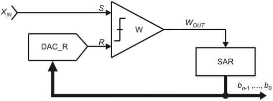
Figure 4.
Simplified model of the oscillating successive approximation converter.
The equivalent of the measured input value XIN is represented by the n-bit digital output word bn−1, …, b0. At the i-th step of the conversion process, for i = 2, 3, …, n + 1 (except the first step), one bit bi is evaluated, starting from the most significant bit bn−1. If the reference signal R is not greater than the source signal S, the bit bn−i + 1 is set to logic “1”. Otherwise, the bit bn−i + 1 is set to logic “0”.
One of the most distinctive features of the OSA variant is necessity of removing specific reference element Rk (Figure 2c) in case of overestimation (Figure 2b). This subtraction means a change of the previously made decision. Obviously, such operation is not always possible during the conversion process. Considering a specific case, when the measured input value XIN is non-removable, non-decremental physical quantity, the reference elements Rn−1, …, R0 are also non-decremental. An example of such measured physical quantity XIN is time interval for which the reference elements Rn−1, …, R0 are also non-decremental time units. In such case the time reference elements Rn−1, …, R0 cannot be directly removed during conversion, because it is impossible to turn back time. Nevertheless, it should be noted that indirect conversion of non-removable values is still possible using the OSA algorithm [6]. It requires an additional preconversion process to replace non-removable value XIN by removable physical quantity (e.g., charge or voltage).
2.2. Full-Scale Monotonic Successive Approximation
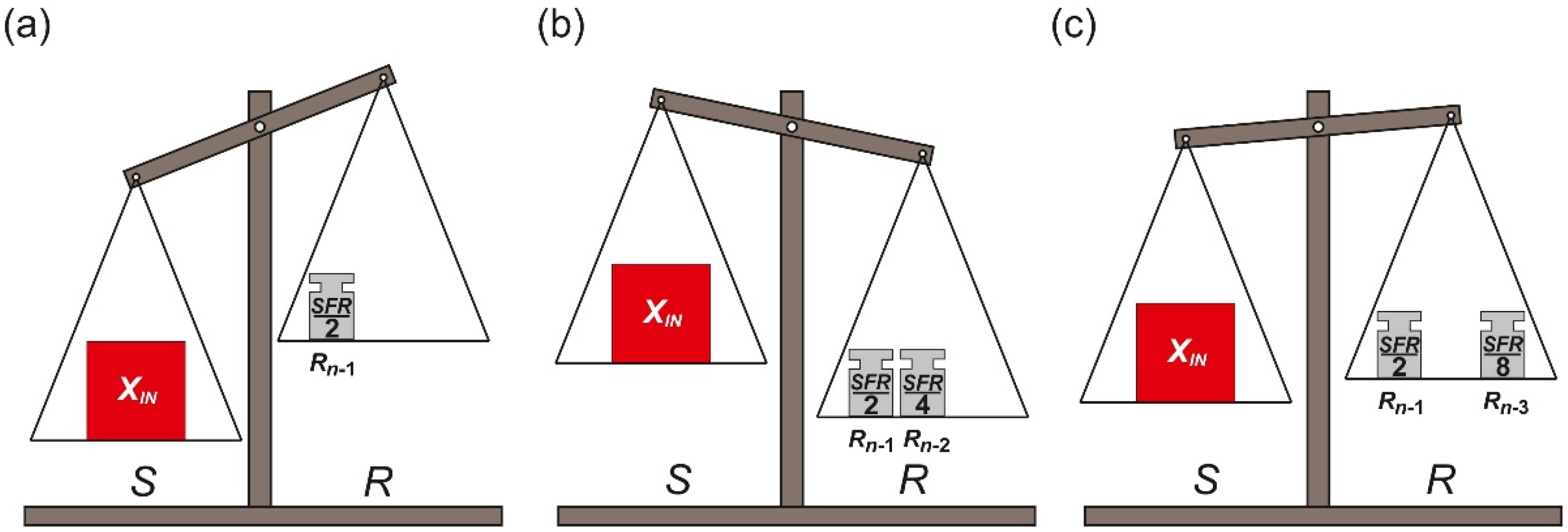
The necessity of removal operation, which is associated with the OSA algorithm, does not occur in the second SA variant. The problem is solved by an additional set of binary-scaled reference elements An−1, …, A0 defined as Ak = 2kA0 (Figure 5—white reference weights). Each additional reference element Ak from the set An−1, …, A0 is equal to the appropriate reference element Rk (Ak = Rk) from the set Rn−1, …, R0 (Figure 5—gray reference weights). Similarly to the OSA, the reference elements Rn−1, …, R0 can be placed only on the pan R, but the additional reference elements An−1, …, A0 can be placed only on the pan S.
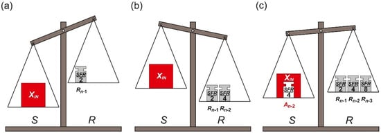
Figure 5.
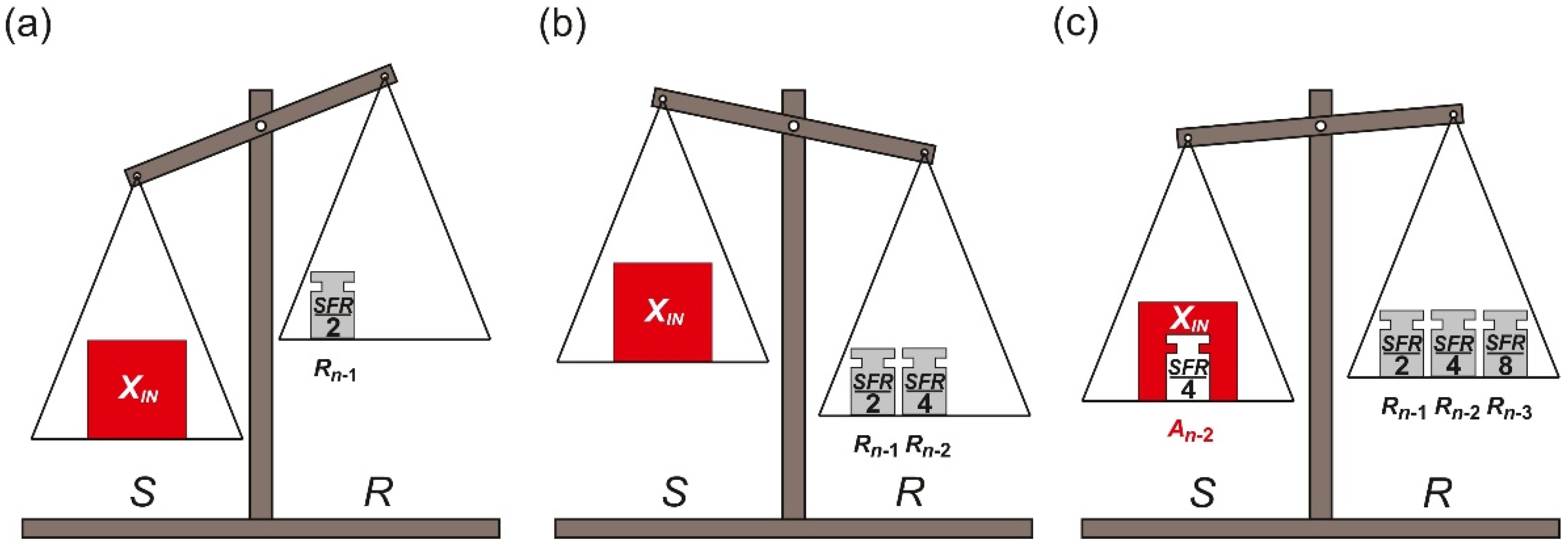
Illustration of full-scale monotonic successive approximation steps: (a) the first step; (b) the overestimation; (c) compensation of the overestimation.
The conversion process starts when the measured input element XIN is placed on the source pan S. Simultaneously, the biggest reference element Rn−1 is placed on the pan R (Figure 5a). At each next step, until the smallest reference element R0 is used, two operations are performed. Firstly, the current state of the pan balance is analyzed. If the total weight of the reference elements currently placed on the pan R is not greater than the total weight of the elements currently placed on the pan S (Figure 5a), no correction is needed at this step. Otherwise, the most recently placed reference element Rk is compensated by the appropriate additional reference element Ak placed on the pan S (Figure 5b,c). Secondly, in both cases, subsequent reference element Rk−1 (k ≥ 1) is placed on the pan R.
When the smallest reference element R0 is used, the conversion is at its final step. The last operation required to accomplish the conversion process is a decision whether to add the additional reference element A0 on the pan S or not.
It clearly follows from the above that all of the reference elements Rn−1, …, R0 are successively placed on the pan R and none of them is removed. On the other hand, the additional reference elements An−1, …, A0 complement the measured input value XIN with the assumption that the total weight on the source pan S has to be contained in range ⟨SFR − R0, SFR). Thus, the measured input value XIN can be evaluated as the difference between the subsets of the reference elements and the additional reference elements placed on the pans:
where Pk indicates if the k-th additional reference element Ak has been placed on the pan S (Pk = 1) or not (Pk = 0). Moreover, at the end of the conversion process the total weight on the pan R always equals (SFR − R0), so the Equation (3) can be rewritten as:
It should be noted that the subtraction in the Equations (3) and (4) is not necessary in order to obtain the correct result. The equivalent of the measured input value XIN can also be expressed as the additional reference elements from the set An−1, …, A0, which remained unused (do not complement the input value XIN on the pan S) at the end of the conversion process:
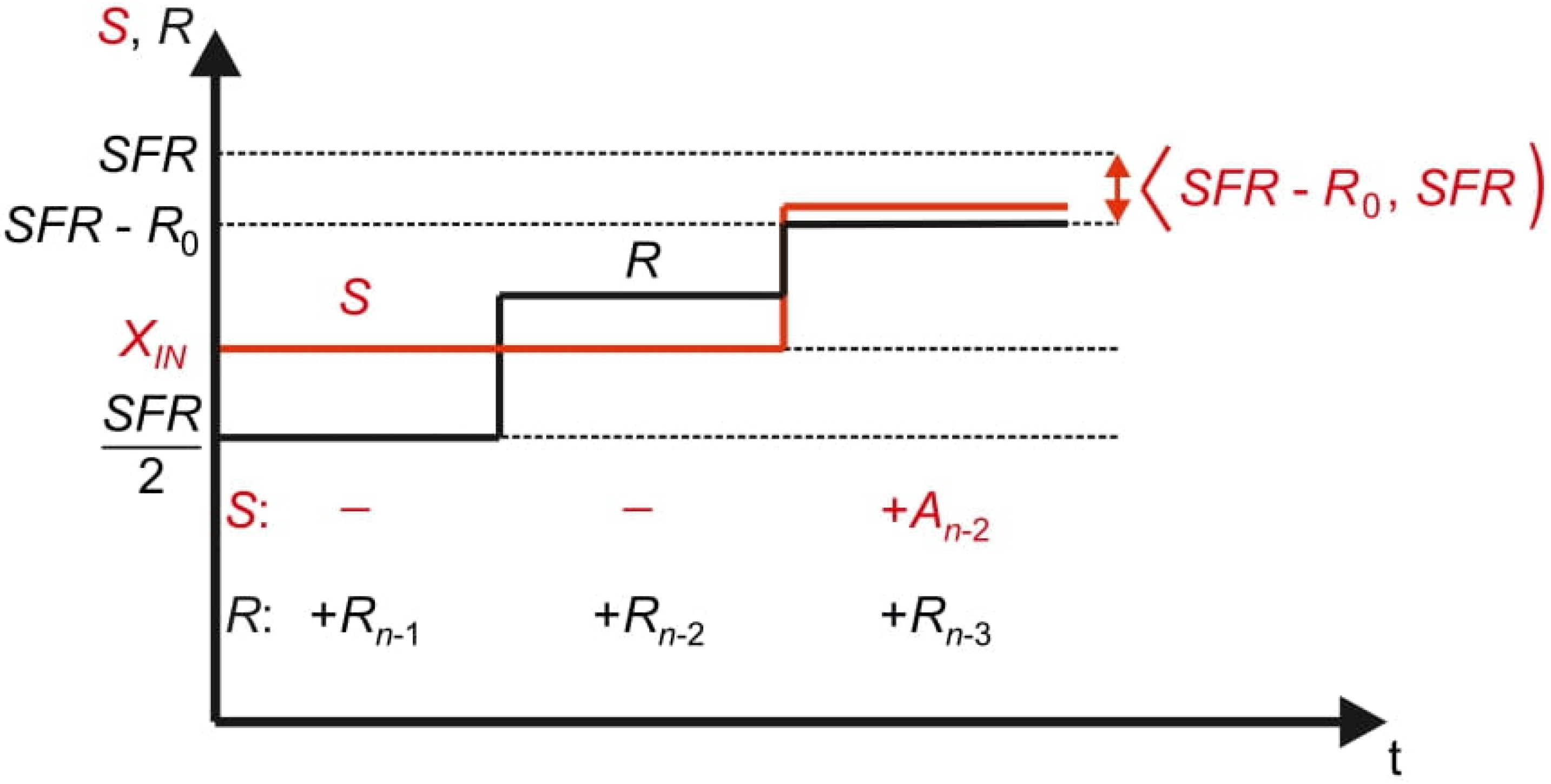
The algorithm ensures that the total weight of each of the pans can only increase, so the removal operation (change of the previously made decision) is unnecessary. The total weight of the elements placed on the pan R will monotonically approach to (SFR − R0) while the total weight of the elements placed on the pan S will be complemented in order to be contained between (SFR − R0) and SFR (Figure 6). Relating to this specific, monotonic character of the functions the name full-scale monotonic successive approximation (FSMSA) is proposed for this algorithm.
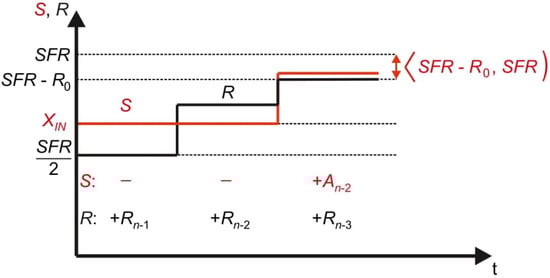
Figure 6.
Full-scale monotonic successive approximation process in the time domain.
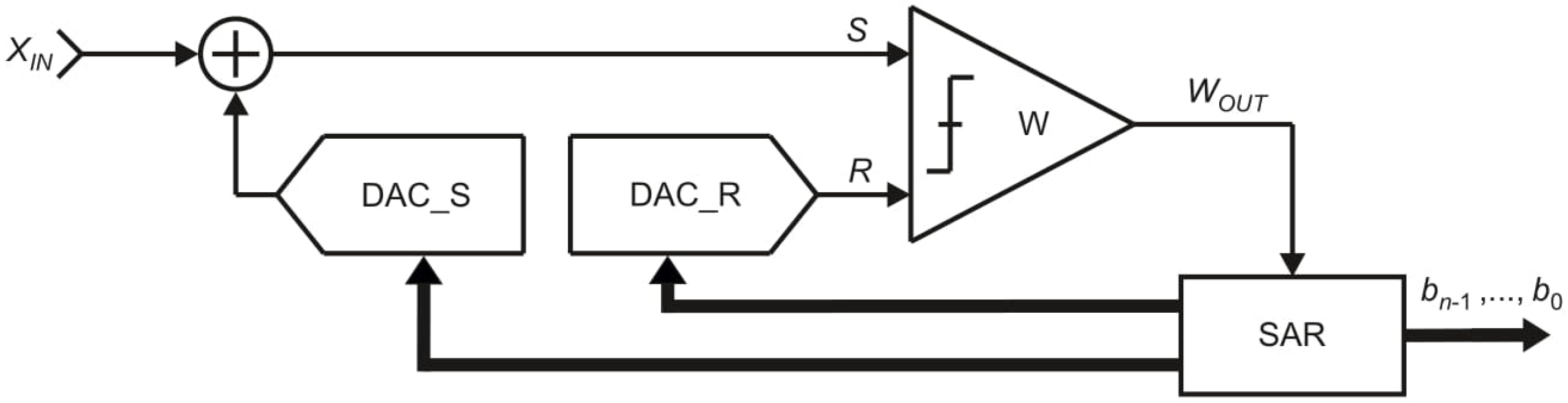
The simplified model of the FSMSA algorithm consists of one comparator W, two digital-to-analog converters—DAC_R and DAC_S—and a control logic block SAR (Figure 7). Similar to the OSA, the digital-to-analog converter DAC_R represents the behavior of the pan R. The additional digital-to-analog converter DAC_S generates the component of the source signal S, which complement the measured input value XIN. The comparator W indicates to the control logic SAR current relation between the source signal S and the reference signal R. Based on this information, the control logic SAR decides whether the value of the source signal S should be increased or not.
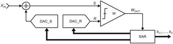
Figure 7.
Simplified model of full-scale monotonic successive approximation converter.
In the FSMSA variant of the SA method, similarly to the OSA, the digital equivalent of the measured input value XIN is represented by the n-bit digital output word bn−1, …, b0. During the conversion process, based on the output value WOUT of the comparator W, the subsequent bits bn−1, …, b0 are evaluated. At the i-th step of the conversion process (i = 2, 3, …, n + 1), if the reference signal R is not greater than the source signal S, the bit bn−i + 1 is set to logic “1”. Otherwise, the bit bn−i + 1 is set to logic “0”.
As it has been shown, the FSMSA variant does not require removal operation. It means that once made decision does not have to be changed in order to acquire the right equivalent of the measured input value XIN. This feature was achieved, among others, by using the additional set of the reference elements An−1, …, A0. When the measured input value XIN is overestimated (S < R), the appropriate element from the additional reference set An−1, …, A0 is used for compensation.
Lack of the removal operation allows for direct conversion of non-removable values such as time intervals. In the FSMSA variant the measured time interval XIN need only to be increased by the additional reference elements An−1, …, A0 defined in the time domain. It allows to avoid the necessity of removal operation, which is impossible in case of time measurement. Of course, the usage of the additional reference elements An−1, …, A0 by definition causes an increase in the hardware resources and energy consumption. Nevertheless, the advantage over OSA in the direct conversion ability causes that there are solutions based on the FSMSA variant [7].
2.3. Monotonic Successive Approximation
The third successive approximation algorithm requires, as in case of the OSA, only one set of the reference elements Rn−1, …, R0 to approximate the measured input value XIN. However, similarly to the FSMSA, the reference elements Rn−1, …, R0 can be placed on both pans: S and R. The practical consequence of having just one set of the reference elements Rn−1, …, R0 in combination with the fact that they can be distributed on both pans (S and R) is that a given weight Rk can be used for both estimation (pan R) and compensation of overestimation (pan S).
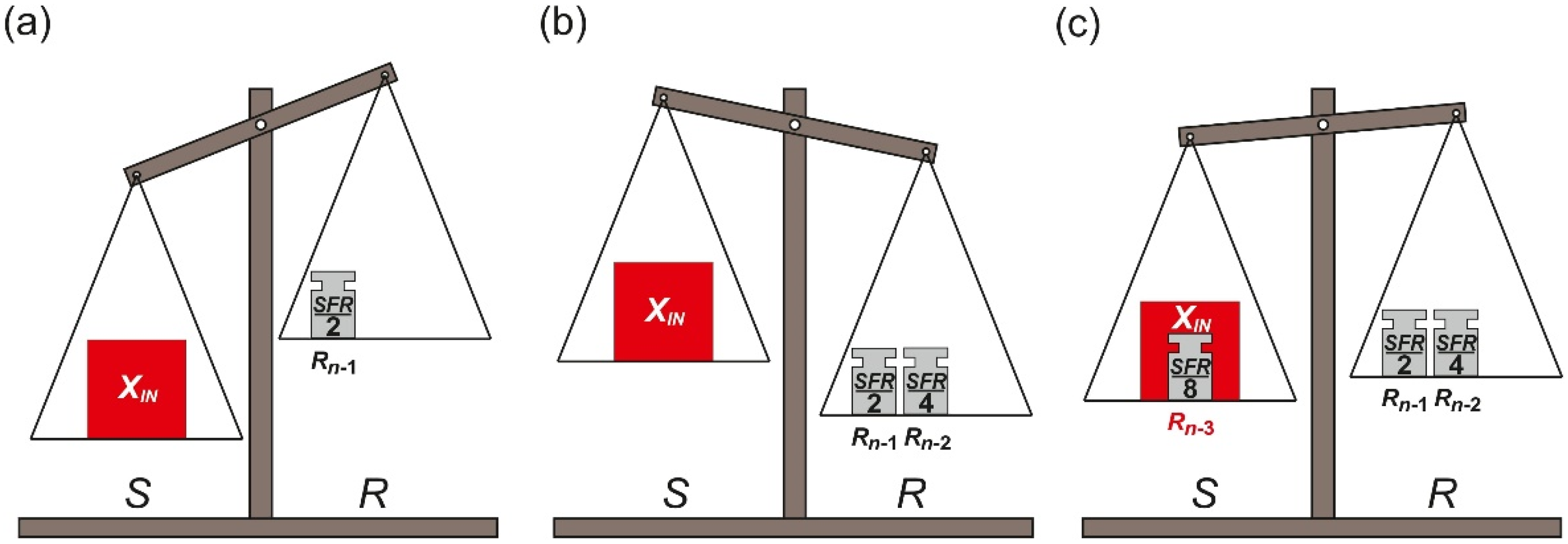
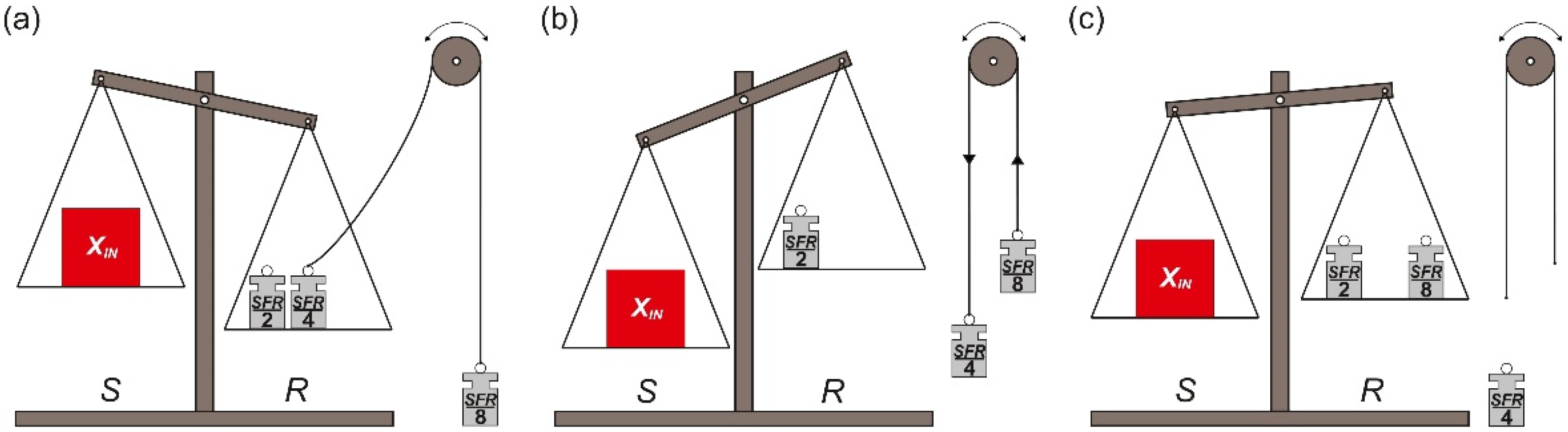
The conversion process starts when the measured input element XIN is placed on the source pan S. Simultaneously, the biggest reference element Rn−1 is placed on the reference pan R (Figure 8a). At each next step, the subsequent reference element Rk (k < n − 1) is placed on the pan (S or R), on which currently accumulated elements weigh less (Figure 8b,c).

Figure 8.
Illustration of monotonic successive approximation steps: (a) the first step; (b) the overestimation; (c) compensation of the overestimation.
The last step of the conversion process is performed once the last reference element R0 is placed on one of the pans. It is limited only to determining the final deflection of the pan balance. This information is used to determine the final result of the conversion process.
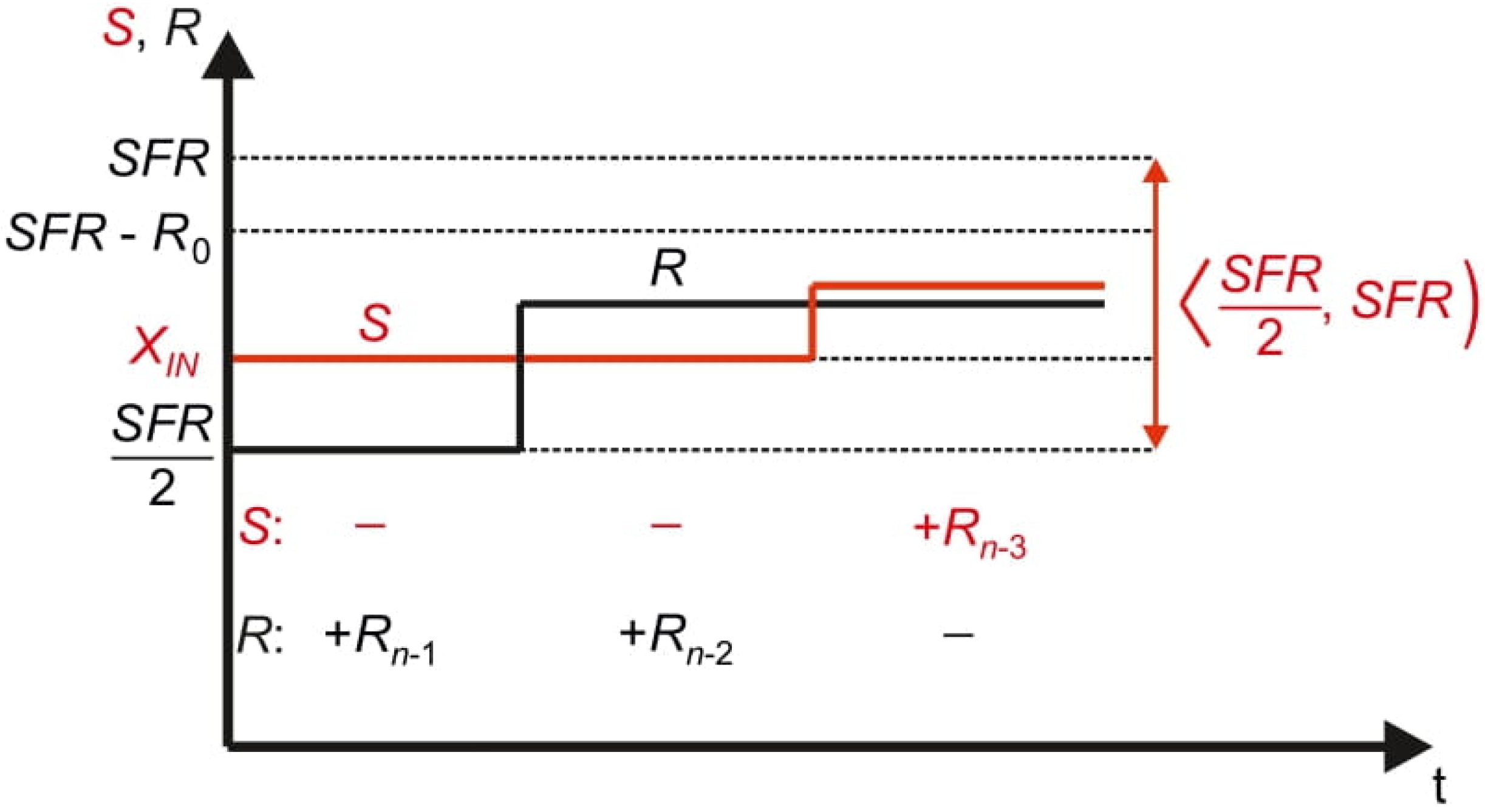
Despite the fact that only one set of the reference elements is used in the conversion process, the removal operation (change of the previously made decision) is unnecessary. The reference elements Rn−1, …, R0 are only added, so the total weight of each pan can only increase. Moreover, during the conversion process, the total weight of each pan approaches to each other monotonically (Figure 9). That is why the name monotonic successive approximation (MSA) is proposed for this algorithm.
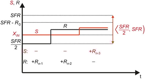
Figure 9.
Monotonic successive approximation process in time domain.
The conversion character of the FSMSA and the MSA variants in some cases may be similar (Figure 6 and Figure 9). Nevertheless, the essential difference of using only one set of the reference elements Rn−1, …, R0 in the MSA causes that the total weight accumulated on each of the pans at the end of the conversion process is always contained between SFR/2 and SFR. The range is relatively wide in comparison to the FSMSA. In that algorithm the total weight accumulated on the pan S at the end of the conversion process varies between (SFR − R0) and SFR, while the total weight on the pan R is equal to (SFR − R0).
At the end of the conversion process the MSA algorithm provides balance between the pans (S and R) with assumed resolution R0. Including the information about the final deflection of the pan balance, the equivalent of the measured input value XIN can be evaluated as:
where Pk indicates if the k-th reference element has been placed on the pan R (Pk = 1) or not (Pk = 0). The final deflection of the pan balance is included in the Equation (6) with Q. If the total weight of the reference elements placed on the pan R is not greater than the total weight of the elements placed on the pan S, Q equals 0. Otherwise, Q equals 1. It should be noted that as in previous binary SA algorithms the digital representation of the measured input value XIN can be successfully obtained without this subtraction [8], which may be suggested by the Equation (6).
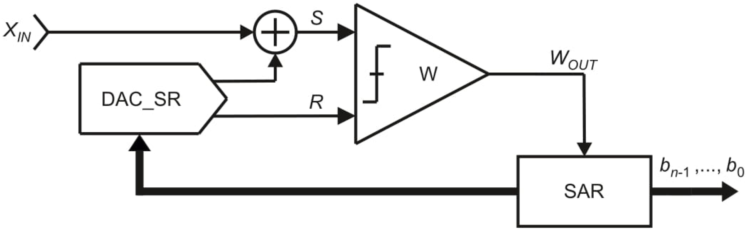
The simplified model of the MSA is presented in Figure 10. It consists of: one comparator W, one digital-to-analog converter DAC_SR with two outputs and a control logic block SAR. Similarly to the previous SA algorithms, the inputs S and R of the comparator W refer accordingly to the pans S and R. The digital-to-analog converter DAC_SR generates the values for both the source signal S and the reference signal R. Based on the output value of the comparator W, the control logic SAR decides which signal: S or R should be increased in the next step.
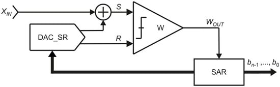
Figure 10.
Simplified model of the monotonic successive approximation.
Similarly to the models of the previously presented SA algorithms, the bits in the digital output word bn−1, …, b0 are evaluated successively, starting from the most significant bit bn−1. At the i-th step of the conversion process (i = 2, 3, …, n + 1), if the reference signal R is not greater than the source signal S the bit bn−i + 1 is set to logic “1”. Otherwise, the bit bn−i + 1 is set to logic “0”.
The MSA algorithm neither requires removal operation (change of the previously made decision) nor the additional set of the reference elements (compensation of the previously made decision). This specific feature is achieved by relatively more complex structure of the circuit (Figure 10). Unnecessity of the removal operation allows for direct conversion of non-removable physical quantities. Therefore, this binary SA algorithm is often used in Time-to-Digital Converters [5,9].
3. Comparison of the Binary Successive Approximation Variants
In the previous sections the description of the binary SA algorithms focused mainly on the ability to direct conversion of non-removable physical quantities. Without a doubt it is a very important aspect of the analog-to-digital conversion, especially from the perspective of time measurement. However, presented models permit the distinction of more differences between presented binary SA algorithms, which also strongly affect the conversion process.
In reference to the previous sections, one of the most evident parameters concerns the number of steps required to determine the equivalent of the measured input value XIN. Obviously, it is directly related to the number of the reference elements Rn−1, …, R0. In all presented binary SA algorithms the number of steps equals (n + 1) for n used reference elements Rn−1, …, R0. Nevertheless, each of the SA algorithms performs different operations within a single step and it must be taken into consideration in order to compare the algorithms reliably.
First of all, the binary SA algorithms use different types of mathematical operations. The OSA uses two types: necessary addition and optional subtraction. For non-removable physical quantities, the optional subtraction, used in case of overestimation (S < R), limits this SA algorithm to indirect conversion only. Of course, possibility of overestimation of the measured input value XIN is an inherent factor of the binary SA and the subtraction is the simplest way to overcome the problem. However, in order to convert directly non-removable values such as time intervals, the subtraction operation cannot occur directly in the SA algorithm.
Eliminating of subtraction results in addition operation (“(−1) (−1) = (+1)”), so in the FSMSA algorithm, instead of optional subtraction, additional operation of addition is used. In result, the FSMSA uses only addition operations during the conversion process, which allows for direct conversion of non-removable values.
Two addition operations can be replaced by one addition operation (“(+1) (+1) = (+1)”). This is applied in the MSA, which uses only one necessary addition operation, but at a cost of a more complicated physical structure (Figure 4, Figure 7 and Figure 10).
The general principle of conversion in the FSMSA and the MSA may seem very similar, because both of the variants compensate the overestimation (R > S) by increasing the source signal S (Sk < Sk + 1) rather than decreasing the reference signal R (OSA variant). However, from the practical point of view, the FSMSA by definition is more expensive. The additional reference elements entail the consequence of using more hardware resources and consuming more energy. On the other hand, controlling one complex digital-to-analog converter (Figure 10) rather than two simple ones (Figure 7) may be more complicated and bring additional problems. Despite the fact the FSMSA is more expensive than the MSA, there are Time-to-Digital Converters solutions based on the variant [7].
The next difference consists in the relation between the measured input value XIN and the characteristics of the reference signal R and the source signal S. In the OSA algorithm, during the conversion process, the measured input value XIN directly affects the value of the reference signal R at each step, while the source signal S is constant and equal to the measured input value XIN. In the FSMSA the reference signal R is totally independent of the measured input value XIN. Its monotonic characteristic is identical in every conversion process. Possible overestimation (S < R) is compensated by the additional reference elements An−1, …, A0, so in this algorithm the source signal S is dependent on the measured input value XIN. In the MSA variant the characteristics of both signals S and R are related to the measured input value XIN as the algorithm uses only necessary addition operation, which can be applied to both signals S and R.
Another parameter, which is differed by the presented models is the last step of the conversion process. For all of the algorithms it is used to evaluate the least significant bit b0 in the digital output word bn−1, …, b0. Even though it is a simple comparison of the source signal S and the reference signal R, it is proceeded within a different operation. The OSA variant compares the signals in order to decide if the reference signal R should be reduced or not. The FSMSA, on the contrary, decides whether the source signal S should be increased. Thus, both of the algorithms check if any last change of the current state is needed. Finally, the MSA does not allow for any additional correction (reduction of reference signal R or increment of the source signal S). The last step of this binary SA variant is reduced to the final comparison of the signals, which determines the value of the least significant bit b0.
Determining the equivalent of the measured input value XIN is also different, which is clearly visible using the pan balance model. In the OSA it is represented by a subset of the reference elements left on the pan R (Equation (2)). There is no necessity of performing any additional mathematical operations. In the FSMSA it can be evaluated as the difference between the total weights of the reference elements accumulated on the pans (Equation (3)). However, at the end of every conversion process the value of the elements accumulated on the pan R is always the same and equal to the sum , so the equation can be simplified to (4). Finally, the MSA not only perform a mathematical operation, but also includes the final deflection of the pan balance (Equation (6)), so in this SA algorithm the evaluation equation is the most complicated. Of course, the above-mentioned expressions just make a comment to the presented pan balance model and in practical implementations of the ADCs there is no need for any further mathematical operations at the end of the conversion. The bits in the output digital word bn−1, …, b0 can be successively evaluated at each step of the conversion process [6,7,10,11].
The application models also differ significantly. From the presented circuits, the OSA model (Figure 4) is the simplest one as the algorithm itself uses relatively simple technique to approximate the measured input value XIN. In the FSMSA algorithm the model is expanded by the additional digital-to-analog converter DAC_S (Figure 7). Such modification increases the capability of the ADCs using this SA algorithm, but at a cost of more demanding implementation. The additional element DAC_S can increase the occupied area of the ADC. In addition, controlling two digital-to-analog converters separately requires more expanded control logic SAR. Finally, the model of the MSA (Figure 10), similarly to the OSA, uses only one digital-to-analog converter DAC_SR, but this element is much more complex, which obviously also directly affects the implementation.
The specific character of each SA method defines the energy required to accomplish the conversion process [12]. In reference to the pan balance model, the consumed energy can be presented in such a way that the energy required to place the reference element Rk or Ak (in case of the FSMSA variant) on the pan balance equals Ek. On the above assumption, the total energy ET required to convert the measured input value XIN using the OSA algorithm equals:
because all of the reference elements Rn−1, …, R0 have to be placed on the pan R regardless of the measured input value XIN. However, as some of the reference elements are placed and in the next step removed, such elements can be used to lift the subsequent reference element (Figure 11). It means that part of the energy can be recovered, so to some extent the OSA can be implemented as an energy-recoverable ADC. A specific implementation of this idea is presented in [13,14,15]. For relatively small measured input value XIN (XIN < R0) the overestimation (S < R) occurs at each step of the conversion process. In such case, the total consumed energy is limited only to the placement of the biggest reference element Rn−1 on the pan R. The energy required to lift each subsequent reference element Rk (k = n − 2, n − 3, …, 0) can be compensated by the previous one Rk+1 (Figure 11b). As a result, the total consumed energy EOSA in the optimized OSA algorithm varies in range:
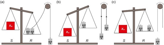
Figure 11.
Illustration of the energy-recovery mechanism in the OSA: (a) the overestimation; (b) energy-recovering compensation; (c) compensated overestimation.
The FSMSA uses two sets of the reference elements and one of them is always fully used (on the reference pan R). The expend of the other subset (used on the source pan S) depends on the measured input value XIN. When it is smaller than the reference element R0 all of the additional reference elements An−1, …, A0 are placed on the pan S at the end of the conversion process. In contrary, if the measured input value XIN is relatively high (XIN ≥ (SFR − R0)), none of the additional reference elements An−1, …, A0 is used. In result, the total consumed energy EFSMSA in the FSMSA algorithm varies in range:
The MSA, as the OSA, uses only one set of the reference elements Rn−1, …, R0. However, as in the FSMSA, none of the reference elements Rn−1, …, R0 is removed during conversion process. In result, regardless of the measured input value XIN, the amount of consumed energy EMSA in the MSA variant always equals:
The above Equations (8)–(10) show that the maximum of the energy EOSA consumed by the optimized OSA is equal to the minimum of the energy EFSMSA consumed by the FSMSA variant. It stems from the fact that the FSMSA uses the additional set of the reference elements An−1, …, A0. The MSA consumes always the same amount of energy, which is exactly equal to the maximum of EOSA and the minimum of EFSMSA. Furthermore, the value of EMSA is the only one, which EOSA and EFSMSA have in common. It is a consequence of including selected OSA and FSMSA properties in the MSA algorithm.
The above conclusions are summarized in the table below (Table 1):

Table 1.
Comparison of the binary SA algorithms.
4. Conclusions
In this paper three algorithms of the binary successive approximation method have been distinguished. The following names, relating to their properties, have been proposed: oscillating successive approximation (OSA), full-scale monotonic successive approximation (FSMSA) and monotonic successive approximation (MSA). The distinction was introduced in order to indicate the main differences between the algorithms, which directly affect the final application.
Undoubtedly the most common successive approximation algorithm is the OSA variant. In addition, it is often incorrectly considered to be the only one. The most important difference between the SA algorithms consists in the ability to direct conversion of non-removable physical quantities such as time intervals. Both the FSMSA and the MSA variants are capable of performing such operation, while in case of the OSA it is impossible. Nevertheless, as mentioned above, conversion of the non-removable values applied as the OSA variant is still possible using indirect conversion. Unfortunately, this entails the necessity of extending the whole conversion procedure by prior preconversion process, which is inherently associated with additional measurement error (uncertainty).
Another important issue raised in this paper is the energy demand, which is imposed by the unique character of conversion in each SA variant. It was shown that its general tendency can be successfully estimated using only such simple models.
Presented systematization of the binary SA algorithms, the specific differences between them, and finally the energy consumption allow for correct identification of the applied SA algorithm and its selected properties, which can be essential in some applications.
Author Contributions
Conceptualization, K.J. and D.K.; investigation, K.J., D.K. and J.S.; methodology, K.J., D.K. and M.M. All authors have read and agreed to the published version of the manuscript.
Funding
This research was funded by Polish National Science Centre, grant number UMO-2017/27/N/ST7/02484.
Conflicts of Interest
The authors declare no conflict of interest.
References
- Kester, W. Data Converters Architectures. In The Data Conversion Handbook; Elsevier: Amsterdam, The Netherlands, 2005. [Google Scholar] [CrossRef]
- Seong, K.; Jung, D.-K.; Yoon, D.-H.; Han, J.-S.; Kim, J.-E.; Kim, T.T.-H.; Lee, W.; Baek, K.-H. Time-Interleaved SAR ADC with Background Timing-Skew Calibration for UWB Wireless Communication in IoT Systems. Sensors 2020, 20, 2430. [Google Scholar] [CrossRef] [PubMed] [Green Version]
- Ro, D.; Um, M.; Lee, H.-M. A Soft-Error-Tolerant SAR ADC with Dual-Capacitor Sample-and-Hold Control for Sensor Systems. Sensors 2021, 21, 4768. [Google Scholar] [CrossRef] [PubMed]
- Szyduczyński, J.; Kościelnik, D.; Miśkowicz, M. A Successive Approximation Time-to-Digital Converter with Single Set of Delay Lines for Time Interval Measurements. Sensors 2019, 19, 1109. [Google Scholar] [CrossRef] [PubMed] [Green Version]
- Kościelnik, D.; Miśkowicz, M.; Szyduczyński, J.; Rzepka, D. Optimizing time-to-digital converter architecture for successive approximation time measurements. In Proceedings of the IEEE Nordic-Mediterranean Workshop on Time-to-Digital Converters NoMe TDC, Perugia, Italy, 3 October 2013; pp. 1–8. [Google Scholar] [CrossRef]
- Kościelnik, D.; Miśkowicz, M. Time-to-digital converters based on event-driven successive charge redistribution: A theoretical approach. Measurement 2012, 45, 2511–2528. [Google Scholar] [CrossRef]
- Chung, H.; Ishikuro, H.; Kuroda, T. A 10-Bit 80-MS/s Decision-Select Successive Approximation TDC in 65-nm CMOS. IEEE J. Solid-State Circuits 2012, 47, 1232–1241. [Google Scholar] [CrossRef]
- Abas, M.A.; Russell, G.; Kinniment, D.J. Built-in time measurement circuits—A comparative design study. IET Comput. Digit. Tech. 2007, 1, 87–97. [Google Scholar] [CrossRef]
- Liu, C.-C.; Chang, S.-J.; Huang, G.-Y.; Lin, Y.-Z. A 10-bit 50-MS/s SAR ADC With a Monotonic Capacitor Switching Procedure. IEEE J. Solid-State Circuits 2010, 45, 731–740. [Google Scholar] [CrossRef]
- Abas, M.A.; Russell, G.; Kinniment, D.J. Design of Sub-10-Picoseconds On-Chip Time Measurement Circuit. In Proceedings of the Design, Automation and Test in Europe Conference and Exhibition, Paris, France, 16–20 February 2004; pp. 804–809. [Google Scholar] [CrossRef]
- Kinniment, D.J.; Maevsky, O.V.; Bystrov, A.; Russell, G.; Yakovlev, A.V. On-chip structures for timing measurement and test. In Proceedings of the Eighth International Symposium on Asynchronous Circuits and Systems, Manchester, UK, 8–11 April 2002; pp. 190–197. [Google Scholar] [CrossRef]
- Saberi, M.; Lotfi, R.; Mafinezhad, K.; Serdijn, W.A. Analysis of Power Consumption and Linearity in Capacitive Digital-to-Analog Converters Used in Successive Approximation ADCs. IEEE Trans. Circuits Syst. I Regul. Pap. 2011, 58, 1736–1748. [Google Scholar] [CrossRef]
- Ginsburg, P.; Chandrakasan, A.P. An energy-efficient charge recycling approach for a SAR converter with capacitive DAC. In Proceedings of the 2005 IEEE International Symposium on Circuits and Systems, Kobe, Japan, 23–26 May 2005; pp. 184–187. [Google Scholar] [CrossRef] [Green Version]
- Lee, J.-S.; Park, I.-C. Capacitor array structure and switch control for energy-efficient SAR analog-to-digital converters. In Proceedings of the 2008 IEEE International Symposium on Circuits and Systems, Seattle, WA, USA, 18–21 May 2008; pp. 236–239. [Google Scholar] [CrossRef] [Green Version]
- Stankovic, D.B.; Stojcev, M.K.; Djordjevic, G.L. Power Reduction Technique for Successive-Approximation Analog-to-Digital Converters. In Proceedings of the 2007 8th International Conference on Telecommunications in Modern Satellite, Cable and Broadcasting Services, Nis, Serbia and Montenegro, 26–28 September 2007; pp. 355–358. [Google Scholar] [CrossRef]
- El-Halwagy, W.; Mousavi, P.; Hossain, M. A 79dB SNDR, 10MHz BW, 675MS/s open-loop time-based ADC employing a 1.15ps SAR-TDC. In Proceedings of the 2016 IEEE Asian Solid-State Circuits Conference (A-SSCC), Toyama, Japan, 7–9 November 2016; pp. 321–324. [Google Scholar] [CrossRef]
- Jiang, R.; Li, C.; Yang, M.; Kobayashi, H.; Ozawa, Y.; Tsukiji, N.; Hirano, M.; Shiota, R.; Hatayama, K. Successive approximation time-to-digital converter with vernier-level resolution. In Proceedings of the 2016 IEEE 21st International Mixed-Signal Testing Workshop (IMSTW), Sant Feliu de Guixols, Spain, 4–6 July 2016; pp. 1–6. [Google Scholar] [CrossRef]
- Kościelnik, D.; Miśkowicz, M. A clockless time-to-digital converter. In Proceedings of the 2010 IEEE 26-th Convention of Electrical and Electronics Engineers in Israel, Eilat, Israel, 17–20 November 2010; pp. 000516–000519. [Google Scholar] [CrossRef]
- Al-Ahdab, S.; Mäntyniemi, A.; Kostamovaara, J. Cyclic time domain successive approximation time-to-digital converter (TDC) with sub-ps-level resolution. In Proceedings of the 2011 IEEE International Instrumentation and Measurement Technology Conference, Hangzhou, China, 10–12 May 2011; pp. 1–4. [Google Scholar] [CrossRef]
- Mantyniemi, A.; Rahkonen, T.; Kostamovaara, J. A CMOS Time-to-Digital Converter (TDC) Based On a Cyclic Time Domain Successive Approximation Interpolation Method. IEEE J. Solid-State Circuits 2009, 44, 3067–3078. [Google Scholar] [CrossRef]
- Chen, Q.; Liang, Y.; Boon, C.C. A 6bit 1.2GS/s Symmetric Successive Approximation Energy-Efficient Time-to-Digital Converter in 40nm CMOS. In Proceedings of the 2020 IEEE International Symposium on Circuits and Systems (ISCAS), Seville, Spain, 12–14 October 2020; pp. 1–5. [Google Scholar] [CrossRef]
- Lee, D.J.; Yuan, F.; Zhou, Y. Successive Approximation Register TDC in Time-Mode Signal Processing. In Proceedings of the 2021 IEEE International Midwest Symposium on Circuits and Systems (MWSCAS), Lansing, MI, USA, 9–11 August 2021; pp. 945–948. [Google Scholar] [CrossRef]
- Szyduczyński, J.; Kościelnik, D.; Miśkowicz, M. Dynamic equalization of logic delays in feedback-based successive approximation TDCs. In Proceedings of the 2017 3rd International Conference on Event-Based Control, Communication and Signal Processing (EBCCSP), Funchal, Portugal, 24–26 May 2017; pp. 1–6. [Google Scholar] [CrossRef]

Publisher’s Note: MDPI stays neutral with regard to jurisdictional claims in published maps and institutional affiliations. |
© 2021 by the authors. Licensee MDPI, Basel, Switzerland. This article is an open access article distributed under the terms and conditions of the Creative Commons Attribution (CC BY) license (https://creativecommons.org/licenses/by/4.0/).