
Integrated Pedal System for Data Driven Rehabilitation

 , ,
, , 
Abstract
:1. Introduction
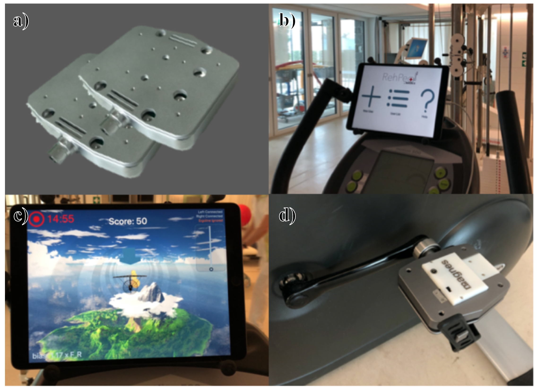
2. Hardware
3. Methods
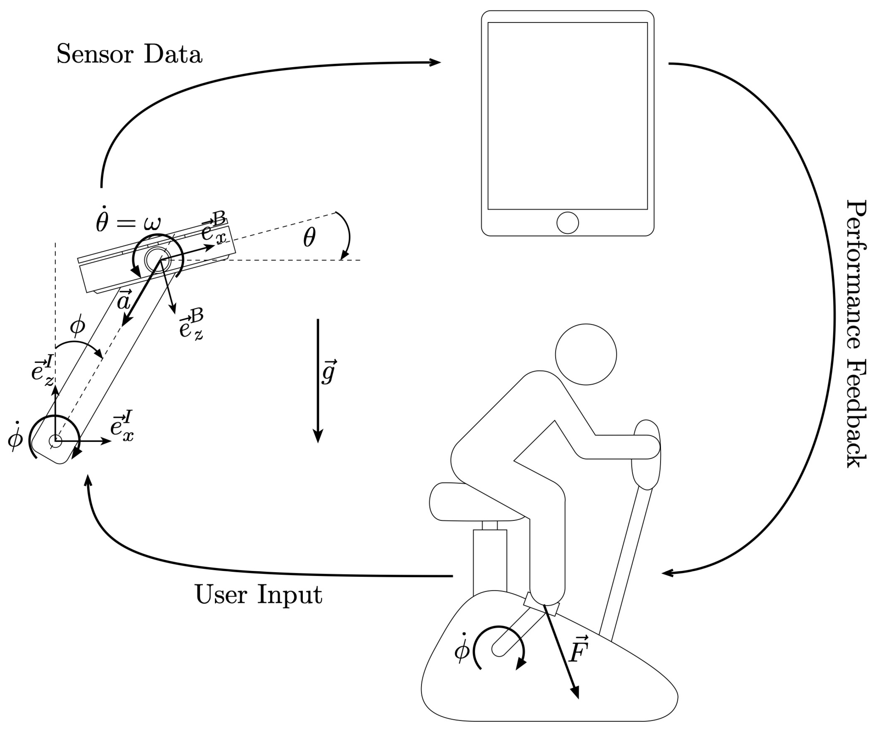
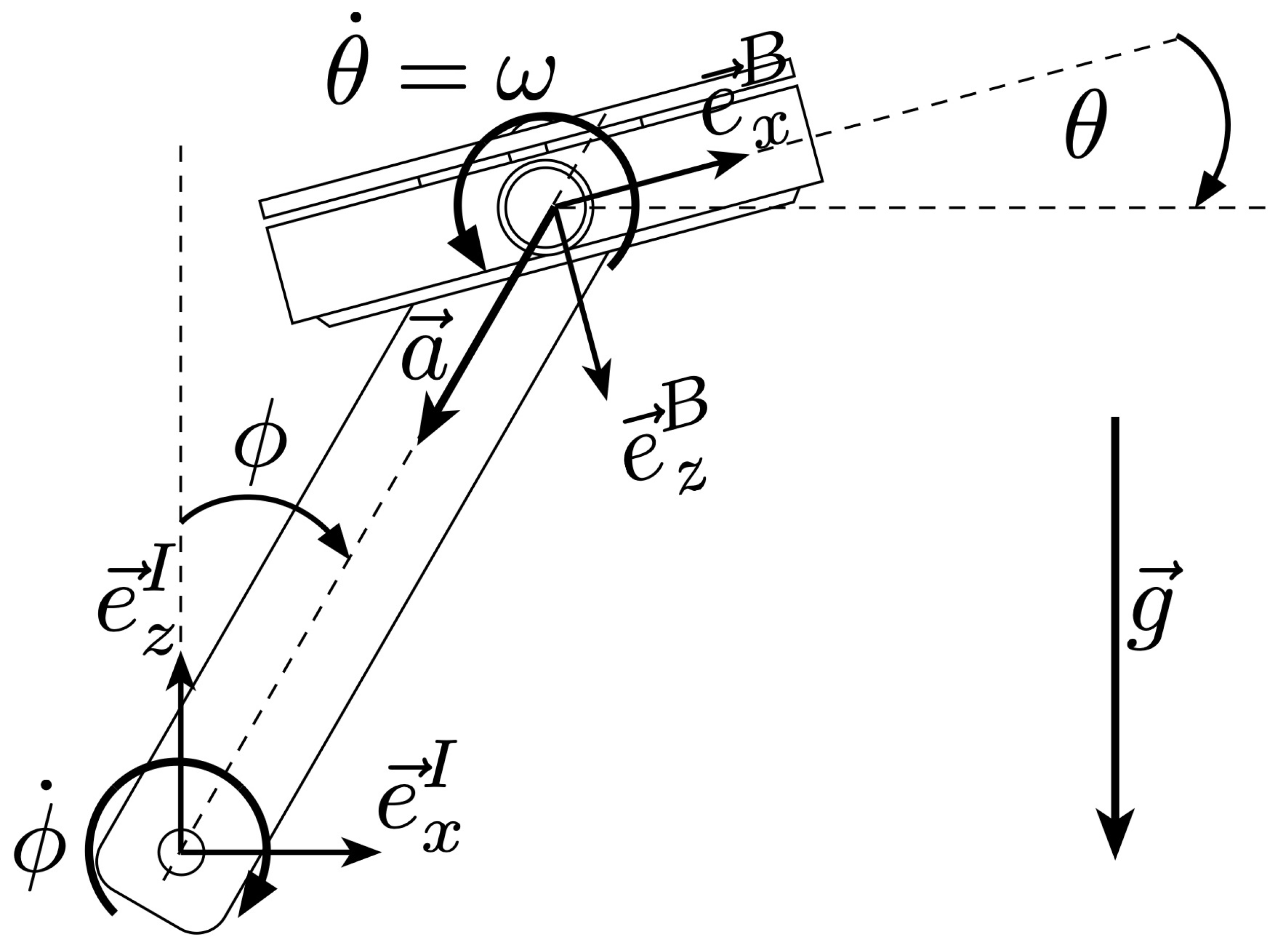
3.1. Definitions and Notation
3.1.1. Crank Angle Definition
3.1.2. Pedal Angle Definition
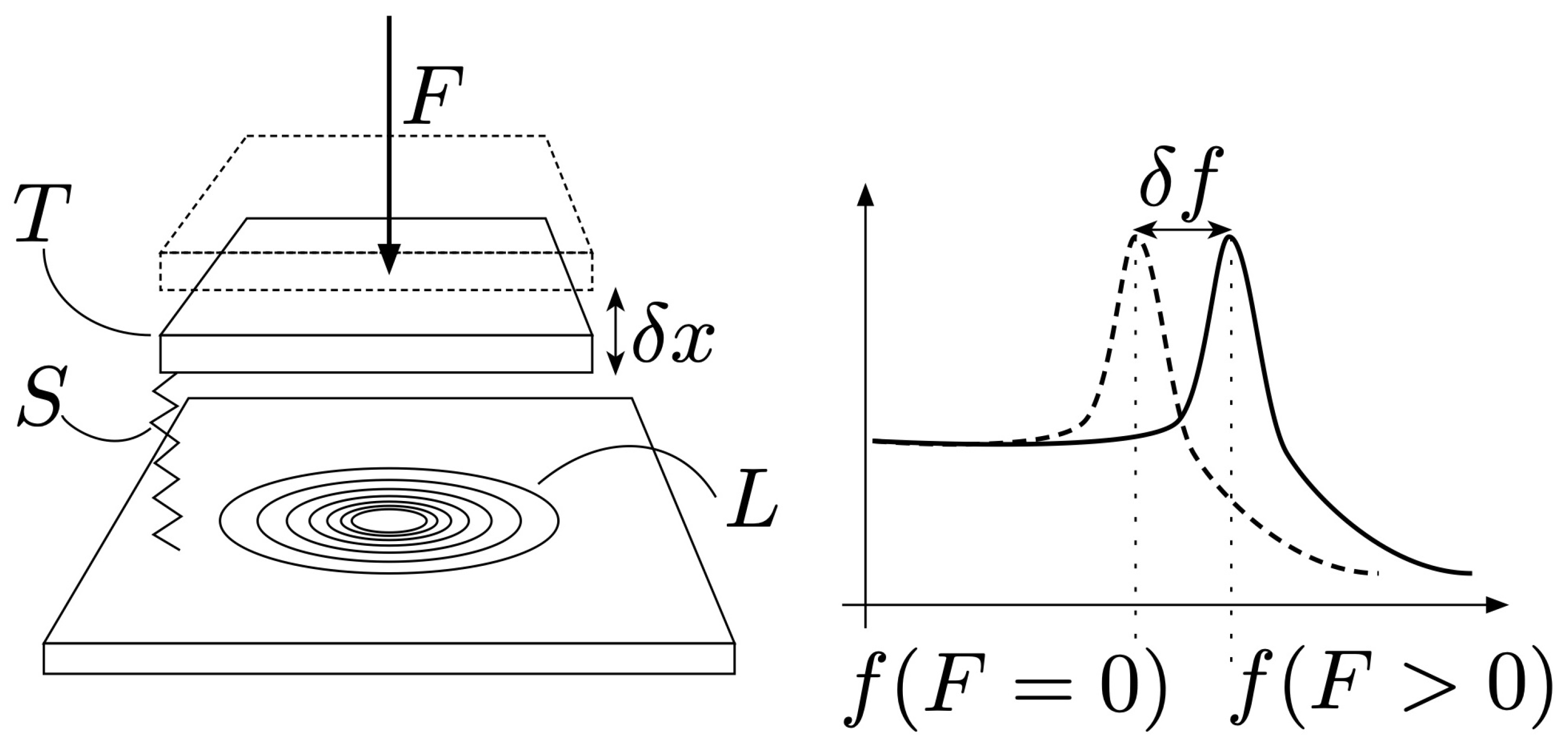
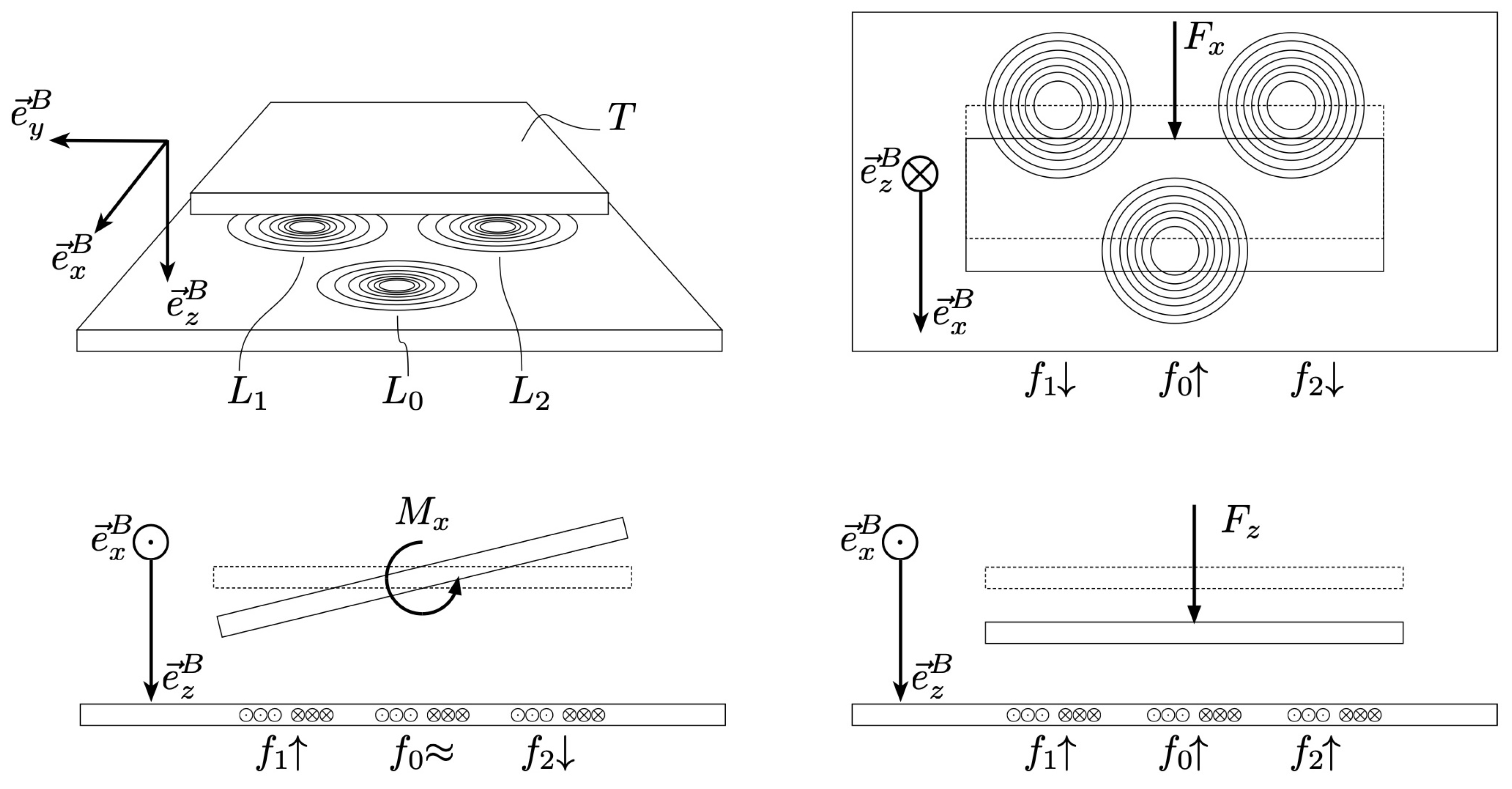
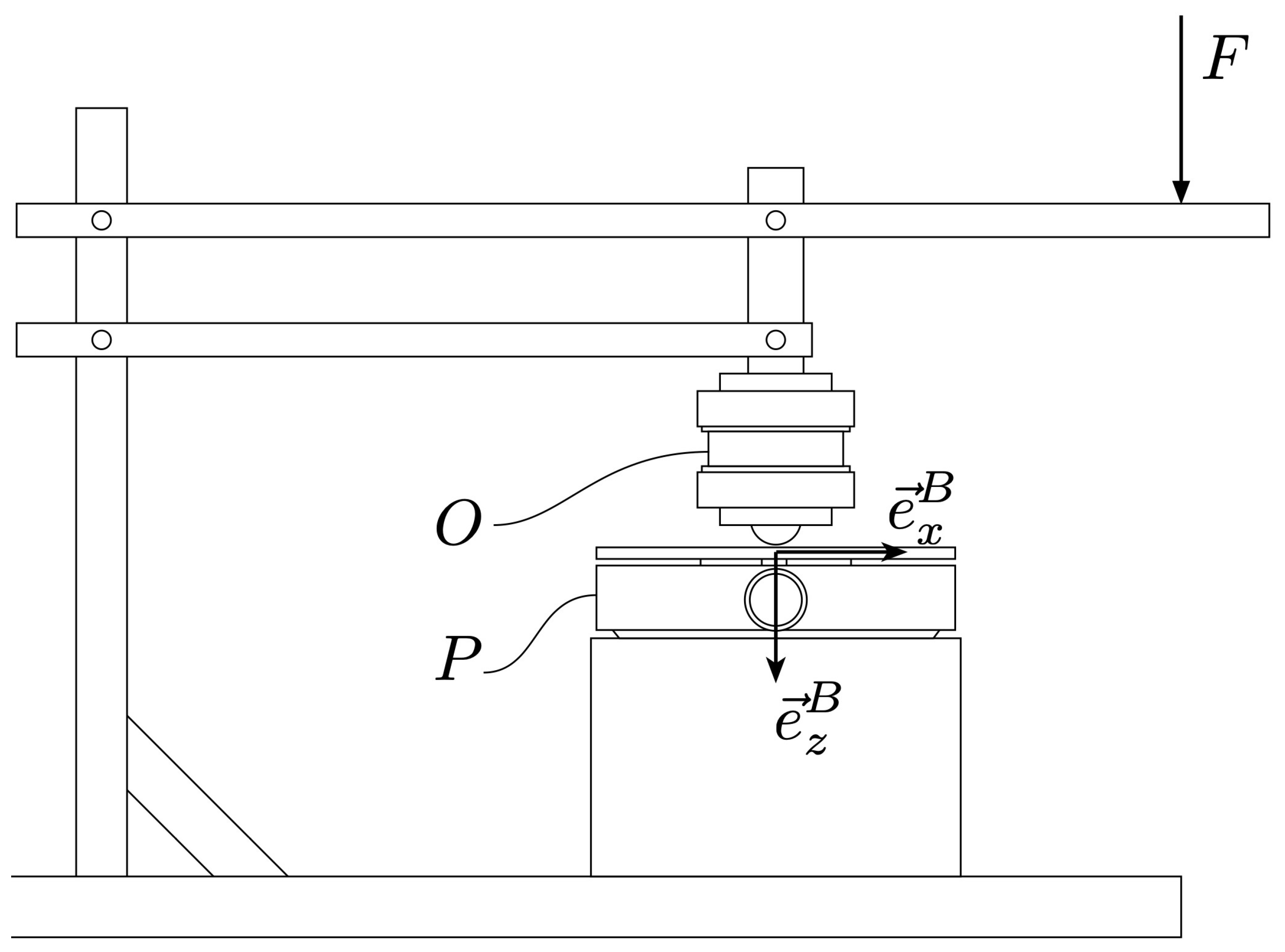
3.2. Load Sensor Calibration
3.3. Pedalling Kinematics
3.3.1. Pre-Processing
3.3.2. Kinematic Model
3.3.3. Crank Angle Estimation
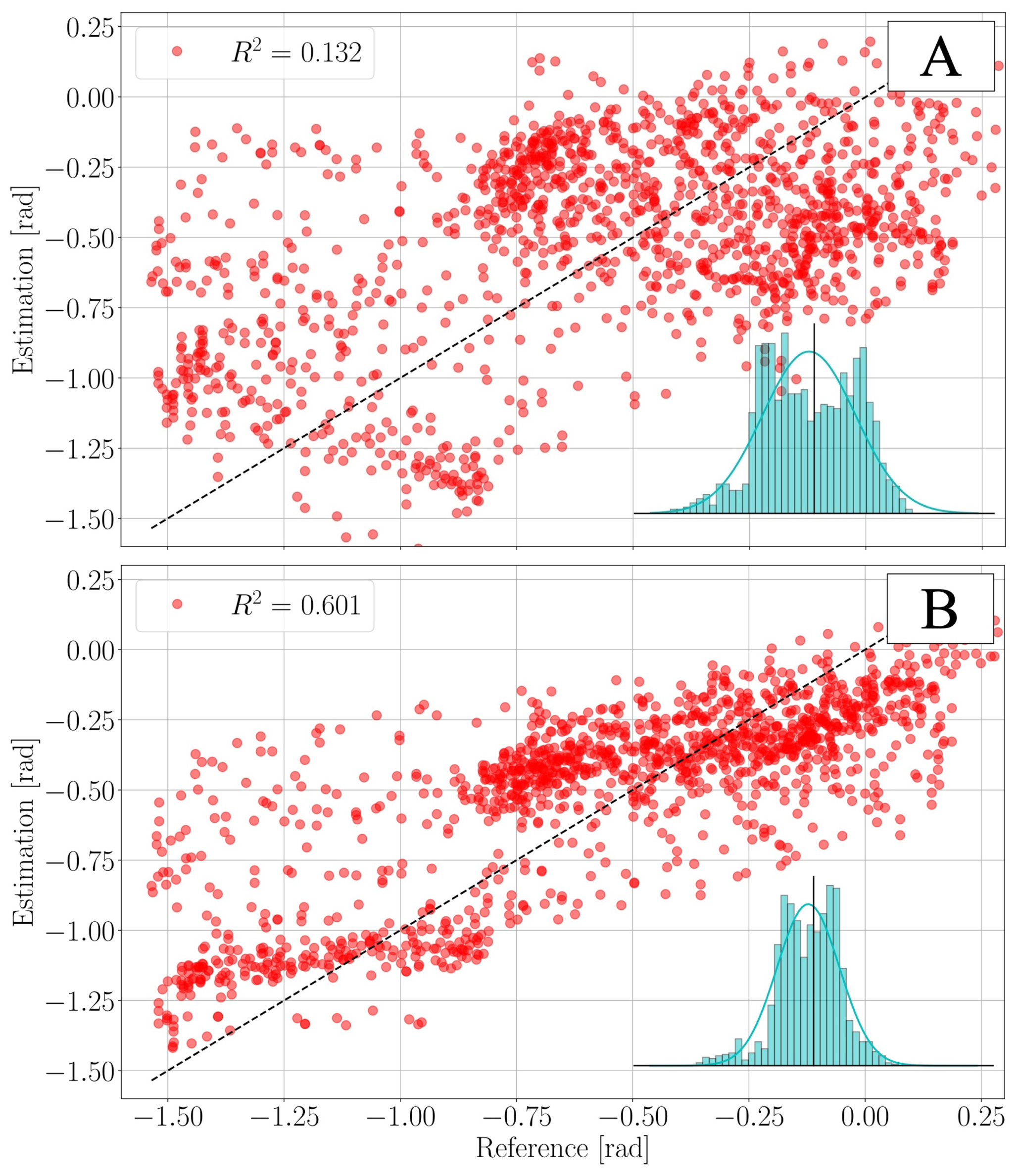
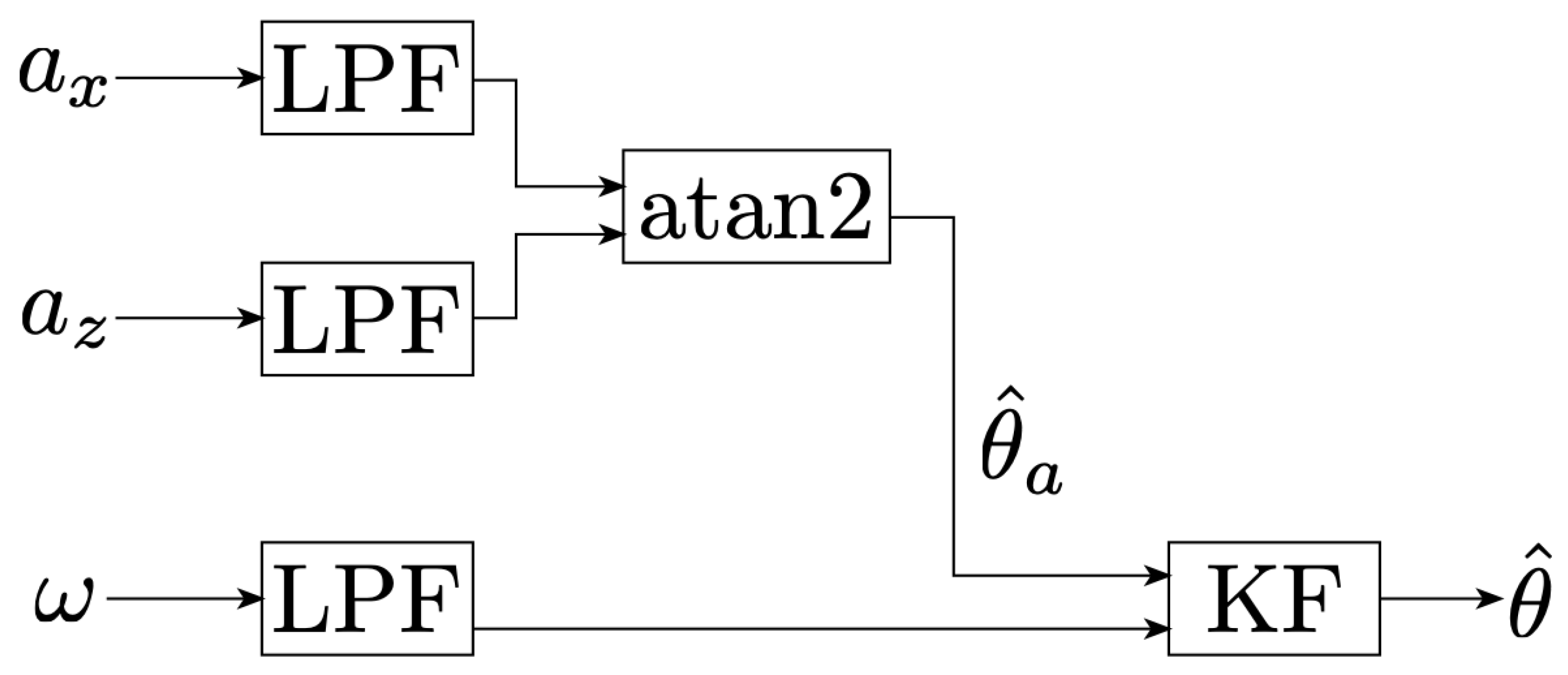
3.3.4. Pedal Angle Estimation
Rough Estimate—Acceleration Angle
Refining the Estimation—Kalman Filter
4. Calibration Results
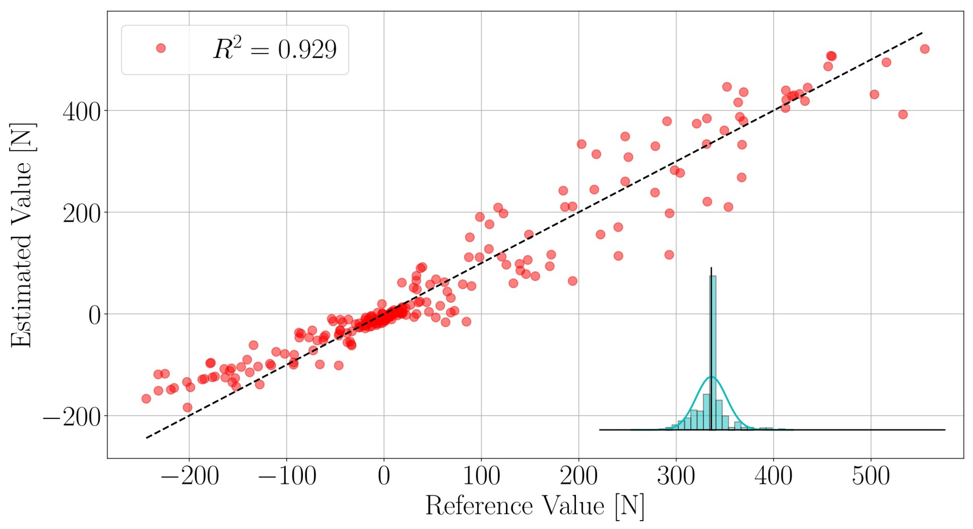
4.1. Load
4.2. Kinematic Parameters
5. Applications
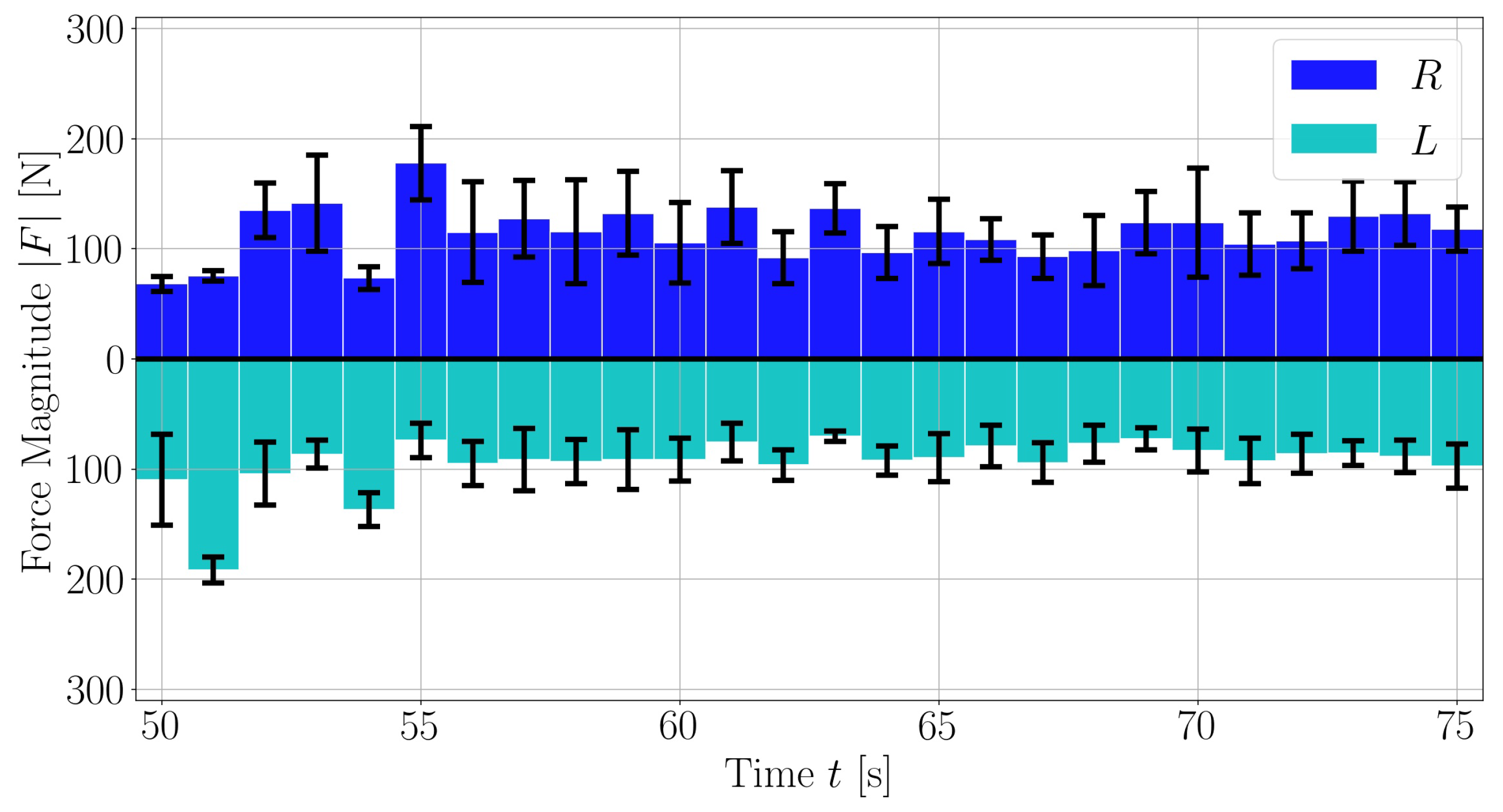
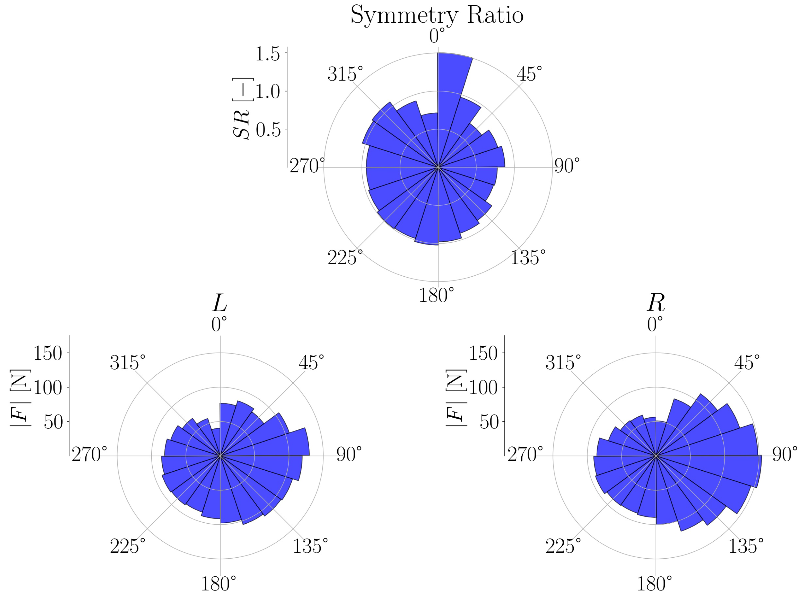
5.1. Data Visualization
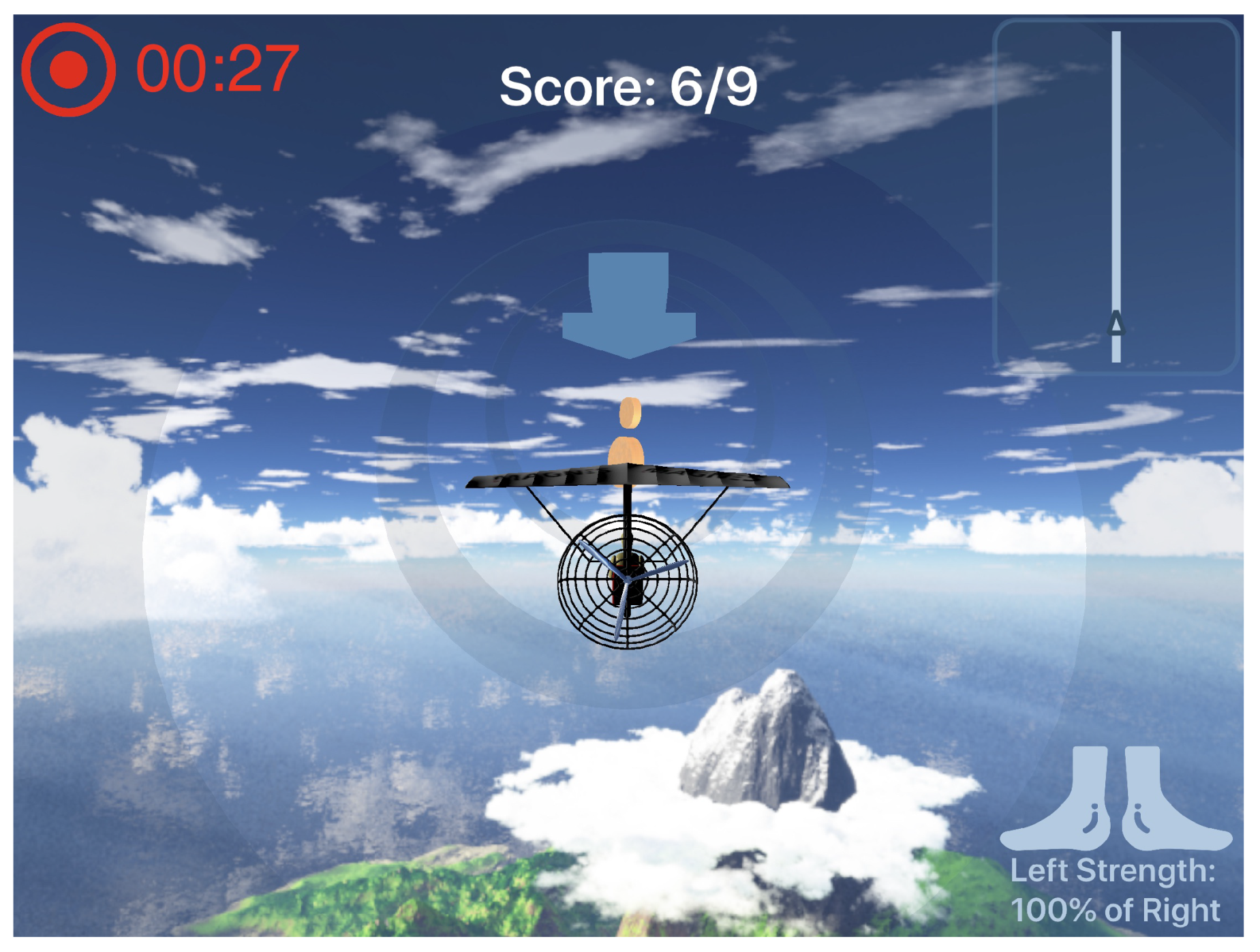
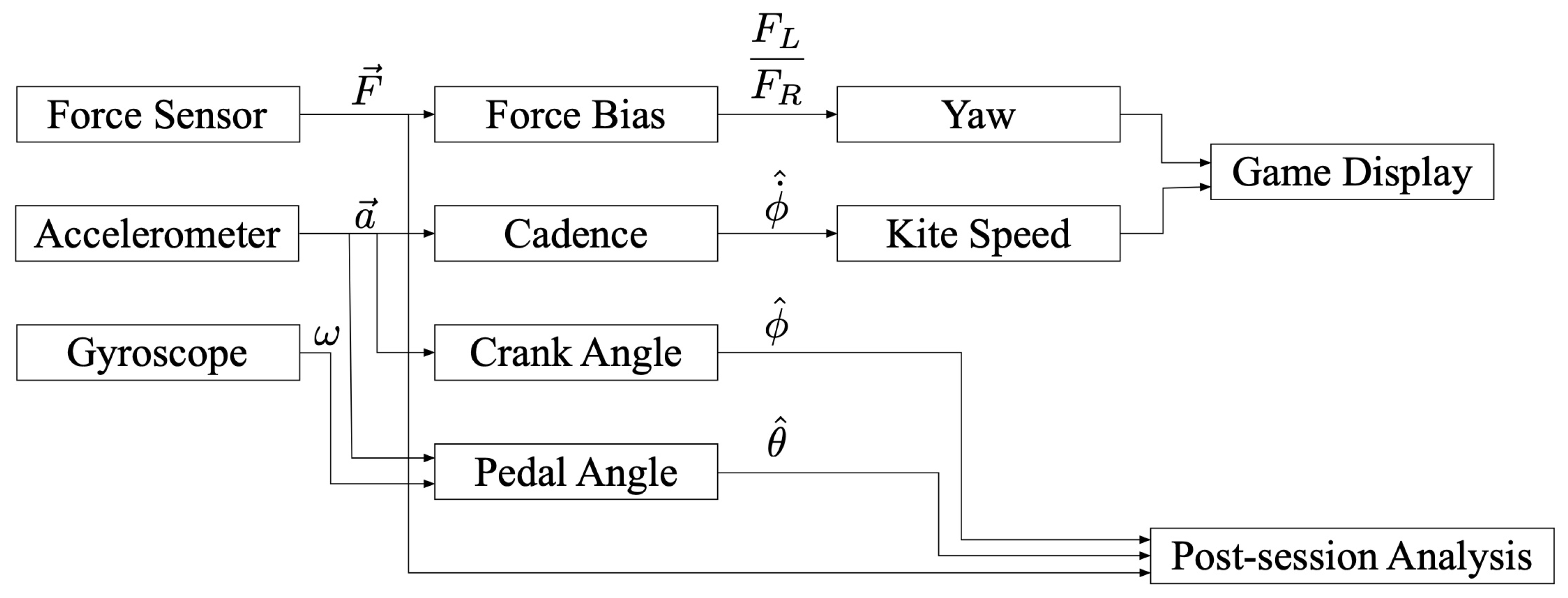
5.2. Gamification
6. Results and Discussion
6.1. Conclusions
6.2. Outlook
Author Contributions
Funding
Institutional Review Board Statement
Informed Consent Statement
Data Availability Statement
Conflicts of Interest
Abbreviations
| BDC | Bottom dead center |
| fps | Frames per second |
| IC | Integrated circuit |
| IMU | Intertial measurement unit |
| KF | Kalman filter |
| LPF | Low-pass filter |
| MAE | Mean absolute error |
| RMSE | Root mean squared error |
| SoC | System on chip |
| TDC | Top dead center |
Appendix A. Derivation of Pedal Kinematics
Appendix A.1. Notation
Appendix A.2. Pedal Kinematics
Appendix A.3. A Note on the Chosen Frames of Reference and the Transformation Matrix R BI
References
- Industry-ARC. Physiotherapy Services Market—Forecast (2021–2026). 2018. Available online: http://xxx.lanl.gov/abs/https://www.industryarc.com/Report/16089/physiotherapy-services-market.html (accessed on 25 September 2021).
- Frontera, W.R. Epidemiology of Sports Injuries: Implications for Rehabilitation; Wiley: Hoboken, NJ, USA, 2003; pp. 3–9. [Google Scholar] [CrossRef]
- Chiarici, A.; Andrenelli, E.; Serpilli, O.; Andreolini, M.; Tedesco, S.; Pomponio, G.; Gallo, M.M.; Martini, C.; Papa, R.; Coccia, M.; et al. An Early Tailored Approach Is the Key to Effective Rehabilitation in the Intensive Care Unit. Arch. Phys. Med. Rehabil. 2019, 100, 1506–1514. [Google Scholar] [CrossRef] [PubMed]
- De Rooij, M.; van der Leeden, M.; Cheung, J.; van der Esch, M.; Häkkinen, A.; Haverkamp, D.; Roorda, L.D.; Twisk, J.; Vollebregt, J.; Lems, W.F.; et al. Efficacy of Tailored Exercise Therapy on Physical Functioning in Patients With Knee Osteoarthritis and Comorbidity: A Randomized Controlled Trial. Arthritis Care Res. 2017, 69, 807–816. [Google Scholar] [CrossRef] [PubMed]
- Bouaziz, W.; Schmitt, E.; Kaltenbach, G.; Geny, B.; Vogel, T. Health benefits of cycle ergometer training for older adults over 70: A review. Eur. Rev. Aging Phys. Act. 2015. [Google Scholar] [CrossRef] [PubMed] [Green Version]
- Veldema, J.; Jansen, P. Ergometer Training in Stroke Rehabilitation: Systematic Review and Meta-analysis. Arch. Phys. Med. Rehabil. 2019, 101, 674–689. [Google Scholar] [CrossRef] [PubMed]
- Ofori, E.K.; Frimpong, E.; Ademiluyi, A.; Olawale, O.A. Ergometer cycling improves the ambulatory function and cardiovascular fitness of stroke patients—A randomized controlled trial. J. Phys. Ther. Sci. 2019, 31, 211–216. [Google Scholar] [CrossRef] [PubMed] [Green Version]
- Mazzocchio, R.; Meunier, S.; Ferrante, S.; Molteni, F.; Cohen, L.G. Cycling, a tool for locomotor recovery after motor lesions? NeuroRehabilitation 2008, 23, 67–80. [Google Scholar] [CrossRef] [PubMed]
- Alankus, G.; Lazar, A.; May, M.; Kelleher, C. Towards Customizable Games for Stroke Rehabilitation. In Proceedings of the SIGCHI Conference on Human Factors in Computing Systems, Atlanta, GA, USA, 10–15 April 2010; pp. 2113–2122. [Google Scholar] [CrossRef]
- Podlog, L.; Heil, J.; Schulte, S. Psychosocial Factors in Sports InjuryRehabilitation and Return to Play. Phys. Med. Rehabil. Clin. N. Am. 2014, 25, 915–930. [Google Scholar] [CrossRef] [PubMed]
- Chana, D.K.C.; Hagger, M.; Spray, C. Treatment motivation for rehabilitation after a sport injury: Application of the trans-contextual model. Psychol. Sport Exerc. 2011, 12, 83–92. [Google Scholar] [CrossRef]
- FECYT—Spanish Foundation for Science and Technology. Video Games to Improve Mobility After a Stroke. 2018. Available online: https://www.sciencedaily.com/releases/2018/02/180214093914.htm (accessed on 25 September 2021).
- Du, W.Y. Resistive, Capacitive, Inductive, and Magnetic Sensor Technologies; CRC Press: Boca Raton, FL, USA, 2015. [Google Scholar]
- Walsh, P.; Mani, D. Inductive Sensing Design Guide. 2019. Available online: https://www.cypress.com/file/427771/download (accessed on 25 September 2021).
- Pedregosa, F.; Varoquaux, G.; Gramfort, A.; Michel, V.; Thirion, B.; Grisel, O.; Blondel, M.; Prettenhofer, P.; Weiss, R.; Dubourg, V.; et al. Scikit-learn: Machine Learning in Python. J. Mach. Learn. Res. 2011, 12, 2825–2830. [Google Scholar]
- Bianchi, G.; Sorrentino, R. Electronic Filter Simulation & Design; McGraw-Hill: Boston, MA, USA, 2007. [Google Scholar]
- Virtanen, P.; Gommers, R.; Oliphant, T.E.; Haberland, M.; Reddy, T.; Cournapeau, D.; Burovski, E.; Peterson, P.; Weckesser, W.; Bright, J.; et al. SciPy 1.0: Fundamental Algorithms for Scientific Computing in Python. Nat. Methods 2020, 17, 261–272. [Google Scholar] [CrossRef] [PubMed] [Green Version]
- Farjadian, A.B.; Kong, Q.; Gade, V.K.; Deutsch, J.E.; Mavroidis, C. VRACK: Measuring Pedal Kinematics During Stationary Bike Cycling. In Proceedings of the 2013 IEEE 13th International Conference on Rehabilitation Robotics (ICORR), Seattle, WA, USA, 24–26 June 2013. [Google Scholar] [CrossRef]
- Kalman, R.E. A New Approach to Linear Filtering and Prediction Problems. J. Basic Eng. 1960, 82, 33–45. [Google Scholar] [CrossRef] [Green Version]
- Bini, R.; Hume, P.; Kilding, A. Optimizing Bicycle Configuration and Cyclists’ Body Position to Prevent Overuse Injury Using Biomechanical Approaches. In Biomechanics of Cycling; Springer: Berlin/Heidelberg, Germany, 2014; pp. 92–107. [Google Scholar] [CrossRef]
- Turpin, N.A.; Watier, B. Cycling Biomechanics and Its Relationship to Performance. Appl. Sci. 2020, 10, 4112. [Google Scholar] [CrossRef]
- Julier, S.J.; Uhlmann, J.K. A New Extension of the Kalman Filter to Nonlinear Systems. In Proceedings of the AeroSense: The 11th International Symposium on Aerospace/Defense Sensing, Simulation and Controls, Orlando, FL, USA, 21–25 April 1997. [Google Scholar]


| Estimate | Load | ||
|---|---|---|---|
| [N] | [N] | [Nm] | |
| 0.772 | 0.929 | 0.937 | |
Publisher’s Note: MDPI stays neutral with regard to jurisdictional claims in published maps and institutional affiliations. |
© 2021 by the authors. Licensee MDPI, Basel, Switzerland. This article is an open access article distributed under the terms and conditions of the Creative Commons Attribution (CC BY) license (https://creativecommons.org/licenses/by/4.0/).
Share and Cite
Schaer, A.; Helander, O.; Buffa, F.; Müller, A.; Schneider, K.; Maurenbrecher, H.; Becsek, B.; Chatzipirpiridis, G.; Ergeneman, O.; Pané, S.; et al. Integrated Pedal System for Data Driven Rehabilitation. Sensors 2021, 21, 8115. https://doi.org/10.3390/s21238115
Schaer A, Helander O, Buffa F, Müller A, Schneider K, Maurenbrecher H, Becsek B, Chatzipirpiridis G, Ergeneman O, Pané S, et al. Integrated Pedal System for Data Driven Rehabilitation. Sensors. 2021; 21(23):8115. https://doi.org/10.3390/s21238115
Chicago/Turabian StyleSchaer, Alessandro, Oskar Helander, Francesco Buffa, Alexis Müller, Kevin Schneider, Henrik Maurenbrecher, Barna Becsek, George Chatzipirpiridis, Olgac Ergeneman, Salvador Pané, and et al. 2021. "Integrated Pedal System for Data Driven Rehabilitation" Sensors 21, no. 23: 8115. https://doi.org/10.3390/s21238115
APA StyleSchaer, A., Helander, O., Buffa, F., Müller, A., Schneider, K., Maurenbrecher, H., Becsek, B., Chatzipirpiridis, G., Ergeneman, O., Pané, S., Nelson, B. J., & Schaffert, N. (2021). Integrated Pedal System for Data Driven Rehabilitation. Sensors, 21(23), 8115. https://doi.org/10.3390/s21238115