Abstract
Global competition among businesses imposes a more effective and low-cost supply chain allowing firms to provide products at a desired quality, quantity, and time, with lower production costs. The latter include holding cost, ordering cost, and backorder cost. Backorder occurs when a product is temporarily unavailable or out of stock and the customer places an order for future production and shipment. Therefore, stock unavailability and prolonged delays in product delivery will lead to additional production costs and unsatisfied customers, respectively. Thus, it is of high importance to develop models that will effectively predict the backorder rate in an inventory system with the aim of improving the effectiveness of the supply chain and, consequentially, the performance of the company. However, traditional approaches in the literature are based on stochastic approximation, without incorporating information from historical data. To this end, machine learning models should be employed for extracting knowledge of large historical data to develop predictive models. Therefore, to cover this need, in this study, the backorder prediction problem was addressed. Specifically, various machine learning models were compared for solving the binary classification problem of backorder prediction, followed by model calibration and a post-hoc explainability based on the SHAP model to identify and interpret the most important features that contribute to material backorder. The results showed that the RF, XGB, LGBM, and BB models reached an AUC score of 0.95, while the best-performing model was the LGBM model after calibration with the Isotonic Regression method. The explainability analysis showed that the inventory stock of a product, the volume of products that can be delivered, the imminent demand (sales), and the accurate prediction of the future demand can significantly contribute to the correct prediction of backorders.
1. Introduction
Backorder occurs when a product is temporarily unavailable or out of stock and the customer places an order for future production and shipment [1]. Backorders are noticed mainly in case of product unavailability due to excessive demand or future release on the market. For instance, COVID-19 and lockdown measures raised the need for antiseptic products and indoor domestic activities that led to a mass wave of online purchases. This trend led to the bullwhip effect, or else the Forrester effect, for many industries and companies that had not succeeded on predicting the increase demand. The stock of products proved insufficient; however, due to products’ low availability and alternative solutions, the customers were willing to wait for their order. Another recent example is the early announcement of the upcoming release in the market of a new product from a famous company. In that case, the company accepts backorders from customers, since the initial production quantity will be insufficient to cover the expected demand for the popular product [1]. The ability of a company to address backorders impacts significantly the company’s revenue, share market price, and customers’ trust [2].
The backorders of products play a crucial role in the management of the inventory, since they affect the total production costs of the whole supply chain. In the literature, various studies addressing the Economic Order Quantity (EOQ) and Economic Production Quantity (EPQ) have been published, taking into account backorders [3,4,5,6]. These approaches include: (i) the coordination and minimization of total costs of the supply chain with backorders [7,8] among other factors, such as with stochastic supply distribution [9,10]; (ii) the inventory problem addressed with backorders [11,12,13,14] and safety stocks [15], multi-objective optimization formulations with fixed backorder, and time-weighted backorder [16], stochastic demand and price discount [17,18], the integration of human errors [19], customers’ preferences [20], or customers’ behavior [21], and from the energy-efficient perspective with the aim to minimize carbon emissions [22]; (iii) fuzzy logic to model the demand or the order quantity for finding the optimal stock quantity [23,24,25]; (iv) heuristic approaches for optimizing the inventory systems [26,27,28].
Due to the importance of backorders and their impact on the whole supply chain costs, studies have been focused on the prediction of inventory backorders. To address the issue of backorders prediction, artificial intelligent techniques have been employed to deal with imbalanced data issues, since the number of products going on backorder is much lower than that of those that are on stock [29]. A machine learning approach was proposed [30] to maximize the expected profit of backorder decisions by integrating the profit-based measure into the prediction model and optimizing the decision threshold. In this context, various machine learning models were evaluated, such as Logistic Regression (LR) and k-Nearest Neighbor (KNN) classifiers, Decision Tree, Support Vector Machine (SVM), and Multi-Layer Neural Network (NN). Another machine learning approach based on Distributed Random Forest and Gradient Boosting Machine learning techniques was presented for predicting the probable backorder scenarios in the supply chain [2]. Unsupervised learning was used to predict backorders by using Deep Autoencoder [29]. Deep neural networks for imbalanced data were proposed for backorder prediction [1]. A case study on the Danish Craft Beer Breweries was presented by using machine learning models for predicting the backorders [31].
The above studies employed machine learning methods to address the backorder prediction problem, whether a product would be backordered or not. However, none of these aimed to explain and interpret the impact of features on the prediction output. To this end, this study focused on developing an explainable machine learning pipeline for: (i) evaluating the performance of well-known machine learning models to predict backorders as a binary classification problem and (ii) interpreting the results by using a post-hoc explainability model (SHAP) on the best performing model. Special notice was given to the treatment of the imbalanced dataset by using an undersampling technique.
2. Materials and Methods
2.1. Dataset
In this study, the publicly available dataset ‘Predict Product Backorders. Can you predict product back orders?’ (https://www.kaggle.com/c/untadta/data (accessed on 1 October 2021)), that was initially created for a competition, was used. In total, 23 features are included in the dataset. Out of the 23 features given in the dataset (Table 1), 15 are numerical, and 8 (including the target variable “went on back order”) are categorical features. The data consisted of 9714 products that were backordered and 1,038,860 that were not.

Table 1.
Dataset description.
2.2. Mehtodology
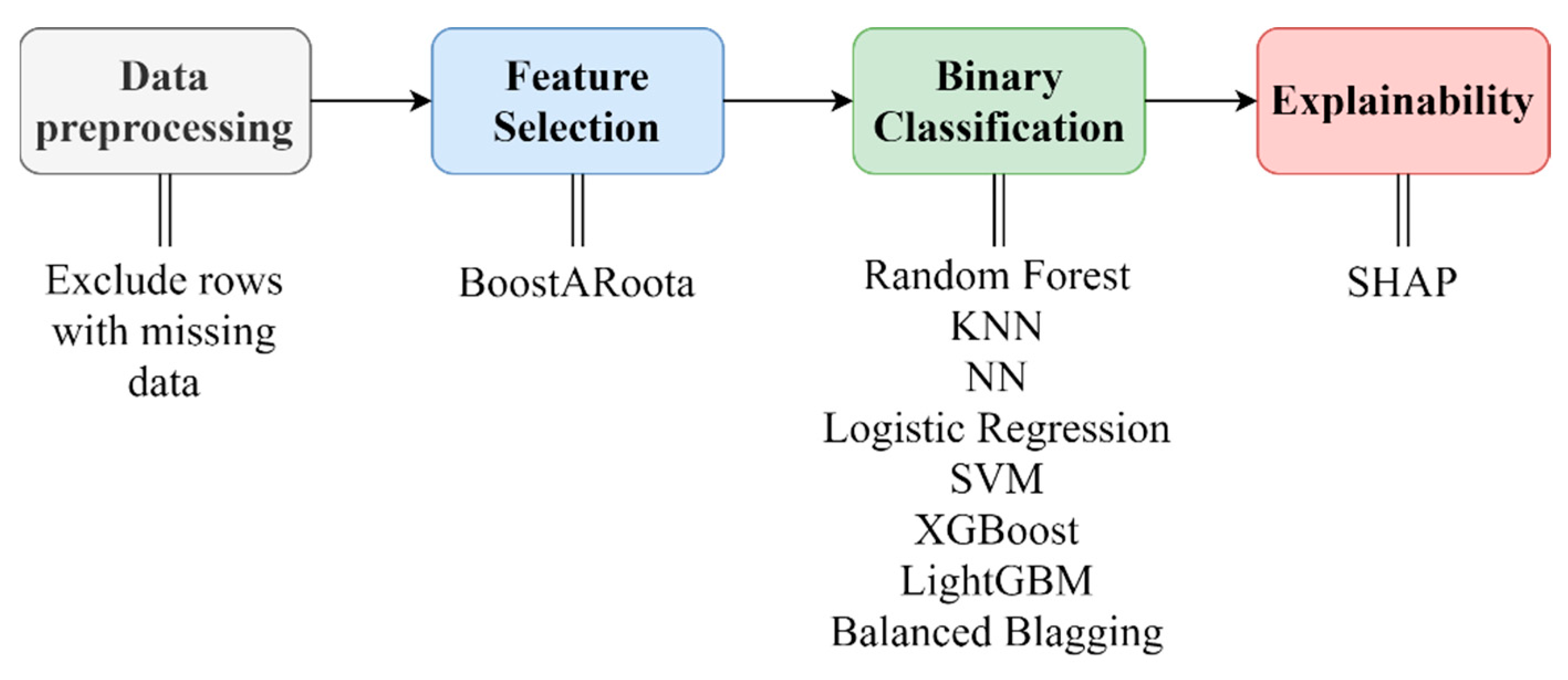
The presented dataset was used in a machine learning (ML) pipeline to predict possible backorders in the inventory management system. The steps integrated in the ML pipeline were the following (Figure 1): (i) data preprocessing to handle the missing data and the categorical values; (ii) feature selection via a state-of-the-art method, called BoostARoota [32,33]; (iii) a comparative evaluation of popular machine learning models, such as Random Forest (RF), LightGBM (LGBM), XGBoost (XGB), Balanced Blagging (BB), Neural Networks (NN), Logistic Regression (LR), Support Vector Machines (SVM), and K-Nearest Neighbors (KNN); (iv) an explainability analysis with the use of the SHAP model applied to the best-performing prediction model in (iii).

Figure 1.
Methodology steps.
For the preprocessing of the dataset, we deleted the rows with missing values, so that we had the maximum possible real information. In addition, we normalized the data set to [0,1]. Finally, to address the problem of imbalanced data, we reduced the samples of the majority class to reach the number of samples in the minority class.
Regarding the feature selection process, the state-of-the-art selection method BoostARoota was used. It is a fast XGBoost wrapper feature selection algorithm that follows the Recursive Feature Elimination approach. It operates similarly to Boruta utilizing XGBoost as the base model. BoostARoota returns an optimal subset of features by eliminating up to 10% of the initial set of features. Its effectiveness has been proven in various applications [32,33]. A 10-fold cross validation was performed for the selection of the most important features.
The comparative evaluation included 8 popular and commonly used classifiers, such as Random Forest (RF) [34], K-Nearest Neighbor (KNN) [35], Neural Networks (NN) [36], Logistic Regression (LR) [37], Balanced Blagging (BB) [38], Support Vector Machines (SVM) [39], XGBoost [40], and LightGBM [41]. A 70/30% validation strategy was employed to generate the training and testing sets with an integrated cross validation strategy that employed grid search for the hyperparameter tunning to avoid overfitting and bias error. In Table 2, a description of the employed hyperparameters is presented. For the performance evaluation of the models, the accuracy, recall, f1-score, precision, AUC metrics were used.

Table 2.
Hyperparameters of the selected ML models.
Following the results from the validation of the models, the classifiers with similar performance were calibrated to increase their performance and identify the best one. Calibration is a post-processing operation, which improves the probability estimation of a model [42,43]. To calibrate the models, the Platt Scaling (sigmoid) [44] and Isotonic Regression [45,46] (isotonic) methods were adopted.
A post-hoc explainability was finally applied on the best performing model based on the SHapley Additive exPlanations (SHAP) model to explain the predictive model and the contribution of the most important features. SHAP is a game theory approach typically employed to explain the output of any machine learning model. It connects optimal credit allocation with local explanations using the classic Shapley values from game theory and their related extensions [47,48,49].
3. Results
In this section, the results of each step of the ML methodology are presented.
3.1. Feature Selection
The BoostARoota algorithm selected the following features as important in random order of appearance:
- national inv
- lead time
- in transit qty
- forecast_3_month
- forecast_6_month
- forecast_9_month
- sales_1_month
- sales_3_month
- sales_6_month
- sales_9_month
- min bank
- pieces past due
- perf_6_month_avg
- perf_12_month_avg
- local bo qty
- deck risk
- ppap risk
3.2. Classification
3.2.1. Validation
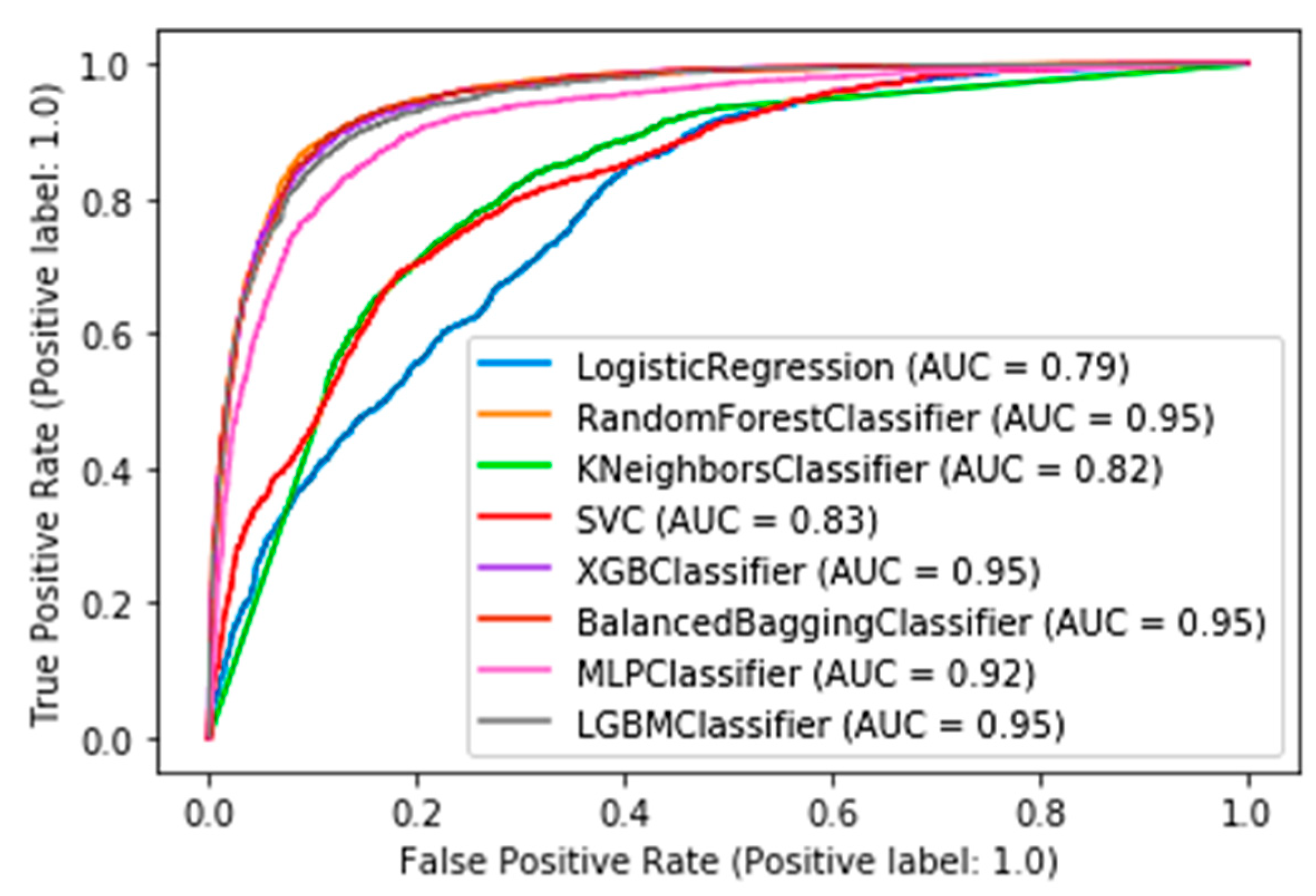
In this subsection, the results from the comparative evaluation of the ML models are presented. Table 3 shows the best metric scores of each classifier used in this study with their hyperparameters tuning. Furthermore, the roc curves and AUC scores are presented in Figure 2.

Table 3.
Best metric scores of each ML model and the selected hyperparameters of each model.

Figure 2.
Roc curves of the competitive ML models.
3.2.2. Calibration
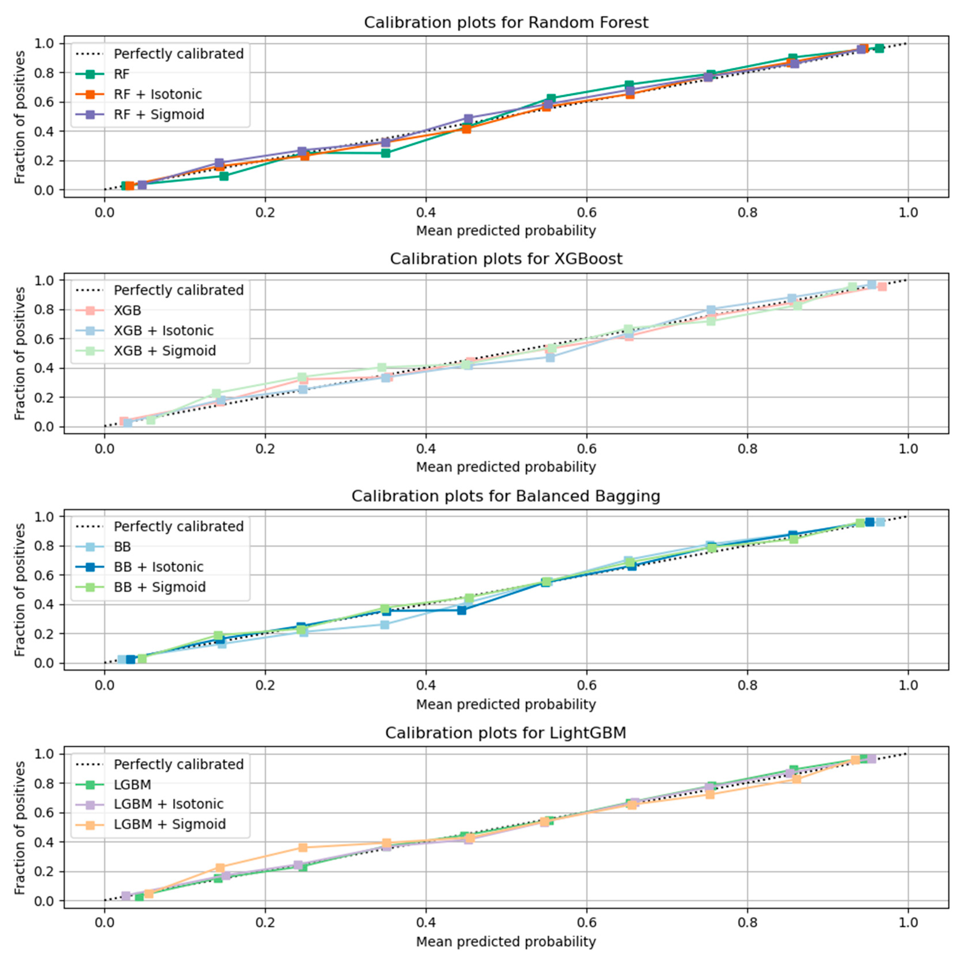
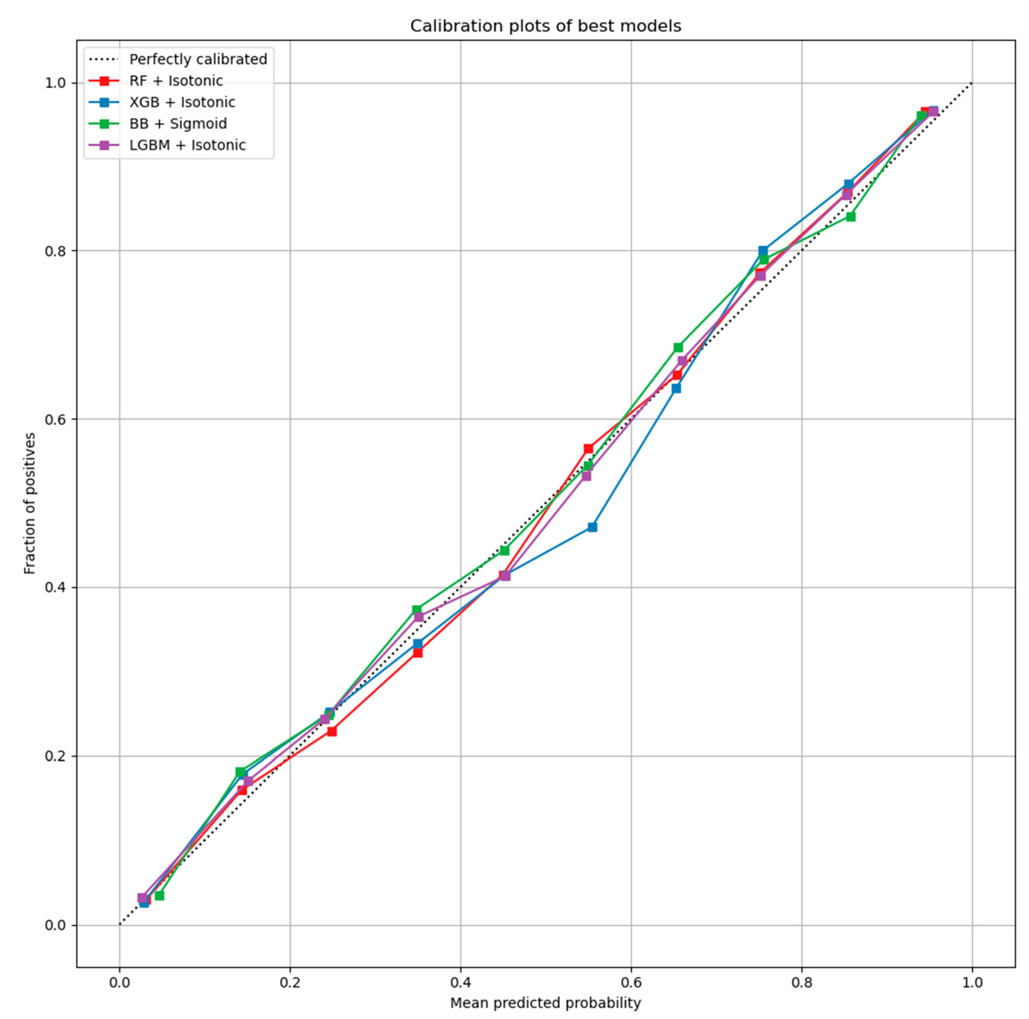
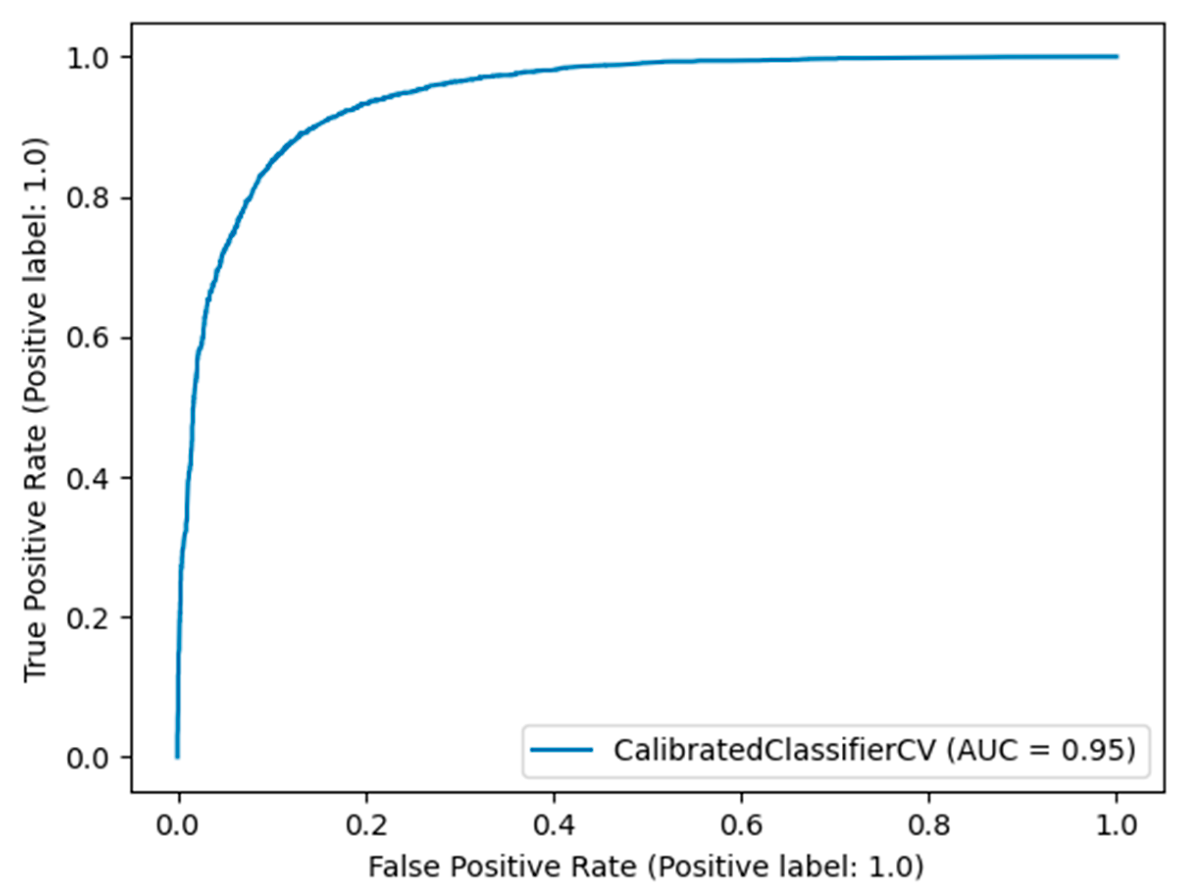
Here, the results from the calibration process are shown. Figure 3 depicts the calibration plots for each of the best performing models that achieved similar performance (RF, LGBM, XGB, and BB). In each plot, the perfectly calibrated line (dot line), the initial model, and the model calibrated with the Platt’s method (sigmoid) and the Isotonic Regression (isotonic) method are presented. For each model, the best calibrated one that best fitted the dot line was then used for a comparison, illustrated in Figure 4. Figure 5 shows the Roc curve of the best overall calibrated model (LGBM + Isotonic).
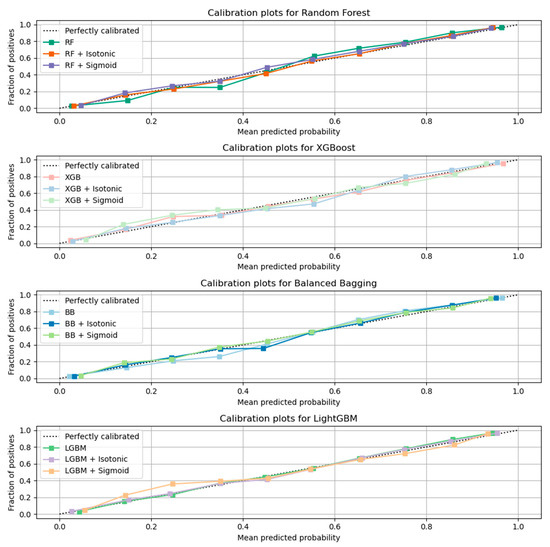
Figure 3.
Calibration results for each classifier with comparative performance based on AUC results.
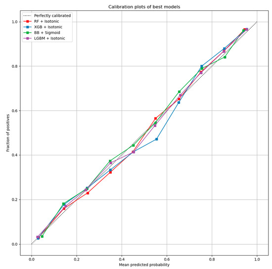
Figure 4.
Best calibrated models for each classifier.

Figure 5.
Roc curve of the LGBM + Isotonic model.
3.3. Explainability
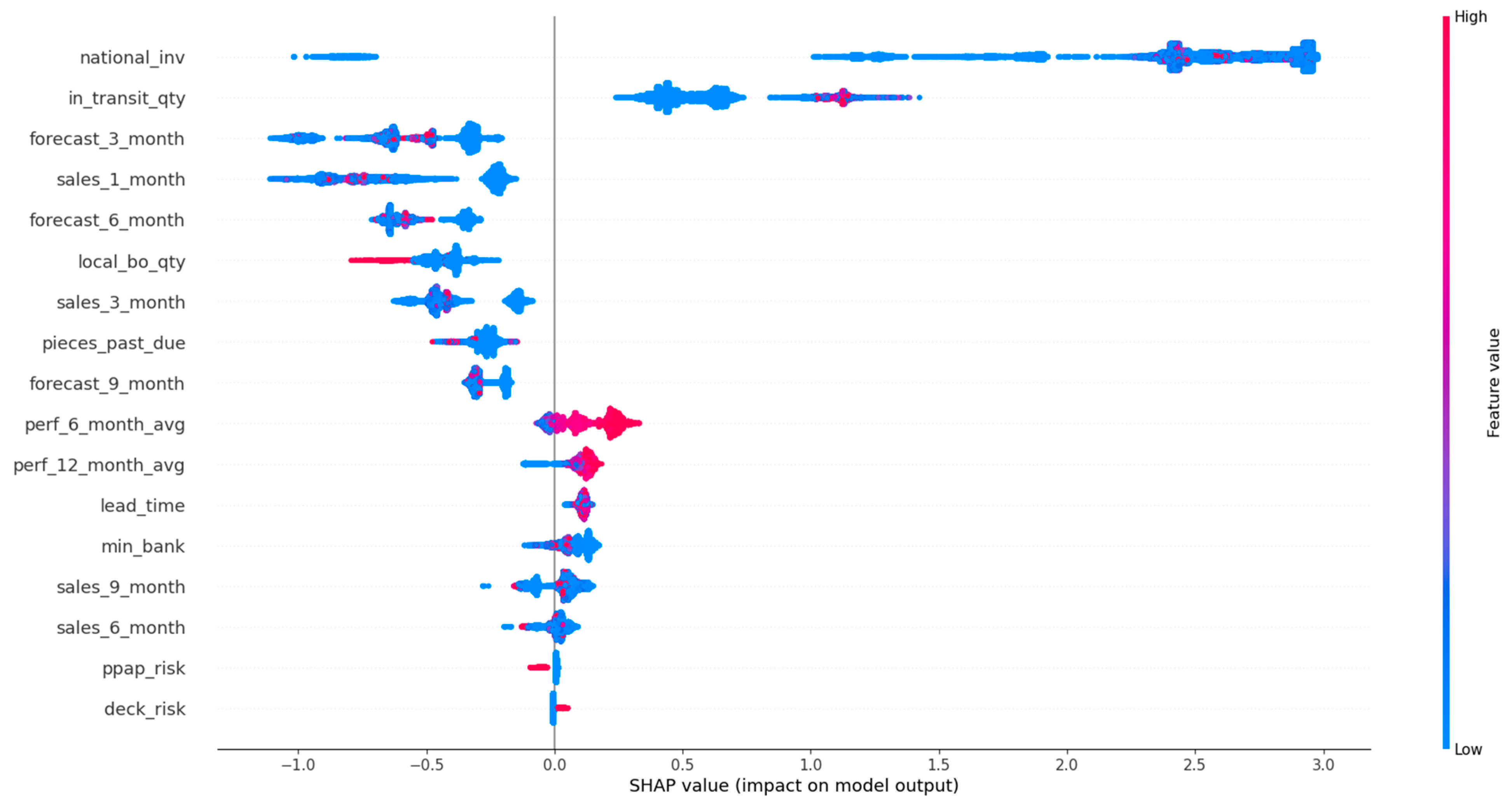
In this section, the results of the SHAP analysis are presented. Figure 6 illustrates the summary plot of LGBM calibrated with the Isotonic Regression method, while in Figure 7, the beeswarm plot for the backordered class is shown. Furthermore, Figure 8 and Figure 9 show two examples for products that were classified correctly as backordered and non-backordered, respectively.
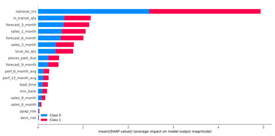
Figure 6.
SHAP summary plot of LightGBM calibrated with the Isotonic Regression method.
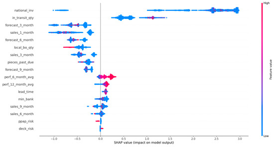
Figure 7.
Beeswarm plot of LightGBM calibrated with the Isotonic Regression method for the backordered class.

Figure 8.
Product correctly classified as non-backordered.

Figure 9.
Product correctly classified as backordered.
4. Discussion
The BoostARoota feature selection method selected 17 out of 23 features that formed the initial dataset. These features were used to form the final dataset for training, validation, and testing of the proposed ML pipeline in this study. They were relevant to inventory stock, transit information, sales forecast, and sales quantity (Section 3.1).
Eight machine learning models were used for a comparative evaluation (Table 3). Among these models RF, XGB, LGBM, and BB presented similar performance based on the AUC score (0.95, Figure 2). Specifically, Table 3 summarizes the metric scores, the confusion matrixes, and the selected hyperparameters of the employed ML models for this binary problem. The majority of the employed classifiers achieved accuracy up to 88.85% in comparison with KNN, LR, and SVM which achieved lower accuracy (up to 75.93%). The RF, XGB, LGBM, and BB models also achieved high performances in the remaining metrics such as recall (up to 90.69%), f1-score (up to 89.12%), and precision (up to 88.10%) scores. From the confusion matrixes of the aforementioned ML models, it turned out that the ML models work satisfactorily in this task.
The RF, XGB, LGBM, and BB models that achieved comparative performance were calibrated based on isotonic and sigmoid methods. Figure 3 illustrates the initial models and their calibration with the aforementioned calibration methods. The results showed that for RF, XGB, and LGBM, the calibration with the Isotonic Regression method reached better results, while for the BB classifier, the Platt Scaling (Sigmoid) method presented better performance. From the comparative evaluation, depicted in Figure 4, the LGBM classifier calibrated with the Isotonic Regression method presented the best overall performance, as it is asymptotically closer to the dotted line that represents the perfectly calibrated model (Figure 4 and Figure 5).
Figure 6 presents the features’ impact on the output of the best model (LightGBM + Isotonic) for the proposed dataset. The features were sorted by the mean absolute value of the SHAP values which represent the SHAP global feature importance. Furthermore, the most important features that significantly affected the prediction output of the model were the national_inv, the in_transit_qty, the forecast_3_month, the sales_1_month, and the forecast_6_month. The national inv concerns the current inventory level of components. The feature in transit qty describes the quantity in transit, and the sales_1_month concerns the sales quantity in the prior month. The features forecast_3_month and forecast_6_month relate to the forecast sales for the next 3 and 6 months.
Figure 8 shows that the topmost influential features n_bank, perf_6_month_avg, in transit, national_inv, sales_1_month, forecast_6_month, sales_3_month, and loval_bo_qty led to the prediction value of 0.35, which was transformed to 1. The features that are indicated with red color influenced positively, which means that they dragged the value closer to 1, while the features in blue color had the opposite effect. Similarly, for an example of a backordered product, Figure 9 shows the values of the top influential features that pushed the product to the backordered class. It is observed that lower values of inventory stock, products’ quantity received, and source performance of the last 6 months and higher values of forecasts and sales pushed the output prediction to the non-backordered class.
To interpret the results from a managerial perspective based on the beeswarm plot illustrated in Figure 7, a product with low stock and high short-term and mid-term future demand will probably be backordered, since the inventory stock will not be able to satisfy the customers’ demand, and at the same time, the expected quantity of products to be delivered to the inventory is also low (Figure 7). Therefore, it is shown that an optimal management of an inventory system that can handle and prevent the forthcoming backorders of products incorporates: (i) accurate predictions on future demands of products, so appropriate decisions can be made on the inventory stock of the product and on product production on time; (ii) increase of the products’ quantity in transit and/or decrease of the transit time by re-scheduling on time the transportation planning and logistics; (iii) the product performance, which means that if the product’s quality satisfies the customers’ requirements, the demand of this product is expected to be increased.
5. Conclusions
Businesses target to increase their profit by retaining low production costs trying in parallel to provide quality service for customer satisfaction. An important part of the production costs is related to the inventory management system. Therefore, it is of high importance to effectively and accurately predict various issues that could occur, leading to additional costs and causing a negative impact on the inventory management system and business operation. One of these issues is product backorder. When a product is backordered, the production should be rescheduled in order to address the demand. This adds additional costs to the business operation. To deal with the backorder issue, this study considered two key aspects: (i) the development of an accurate prediction model for product backorder via a comparative evaluation of popular classifiers and model calibration, and (ii) a post-hoc analysis to explain and interpret the major contributing factors that lead to product backorder.
Specifically, this study tackled the problem of predicting products that will be backordered in an inventory management system. This problem is usually evaluated as a highly imbalanced binary classification problem. Due to the large volume of data, an under-sampling approach was initially adopted to solve this issue. A machine learning pipeline, based on a comparative evaluation of eight popular classifiers, was then adopted, followed by a calibration process applied to the models with similar performance and an explainability analysis of the best-performing model. The results showed that four models achieved almost comparable performance based on AUC scores and other metrics (Table 3). Specifically, the RF, XGB, LGBM, and BB models reached an AUC score of 0.95 (Figure 2). These models were calibrated with the Platt’s and Isotonic Regression methods. The LGBM model calibrated with the Isotonic Regression method presented a slightly better calibration for our data (Figure 4). For this model, post hoc explainability based on the SHAP model showed that the features most contributing to the prediction output of the model relevant to the current inventory level of the component were the quantity in transit and the short-term and mid-term sales quantity and forecast sales (Figure 6). Backorders impact the costs that are linked to production, since the production schedule should be altered in order to deal with the demand of backordered products. Therefore, from the above analysis, it is shown that the decisions that will be made regarding the inventory stock of a product can significantly contribute to the optimal operation of an inventory management system. This decision should be made based on the volume of products that can be delivered, the imminent demand (sales), and the accurate prediction of the future demand.
A limitation of this study is the use of resampling techniques to cope with imbalanced data. To this end, future work will include the use of Siamese neural networks that have proven effective in case of imbalanced datasets.
Author Contributions
Conceptualization, C.N.; methodology, C.N., C.K. and S.M.; software, C.N., C.K.; validation, C.N., C.K. and S.M.; formal analysis, C.N., C.K. and S.M.; data curation, C.N. and C.K.; writing—original draft preparation, C.N. and C.K.; writing—review and editing, C.N., P.K. and S.M.; visualization, C.N. and C.K.; supervision, C.N.; project administration, S.M. and P.K. All authors have read and agreed to the published version of the manuscript.
Funding
This research received no external funding.
Institutional Review Board Statement
Not applicable.
Informed Consent Statement
Not applicable.
Data Availability Statement
The dataset used in this study can be found at https://www.kaggle.com/c/untadta/data (accessed on 23 November 2021).
Acknowledgments
We would like to thank the authors for the public availability of the dataset (https://www.kaggle.com/c/untadta/data (accessed on 1 October 2021)) used in this study.
Conflicts of Interest
The authors declare no conflict of interest.
References
- Shajalal, M.; Hajek, P.; Abedin, M.Z. Product Backorder Prediction Using Deep Neural Network on Imbalanced Data. Int. J. Prod. Res. 2021, 1–18. [Google Scholar] [CrossRef]
- Islam, S.; Amin, S.H. Prediction of Probable Backorder Scenarios in the Supply Chain Using Distributed Random Forest and Gradient Boosting Machine Learning Techniques. J. Big Data 2020, 7, 65. [Google Scholar] [CrossRef]
- Widyadana, G.A.; Cárdenas-Barrón, L.E.; Wee, H.M. Economic Order Quantity Model for Deteriorating Items with Planned Backorder Level. Math. Comput. Model. 2011, 54, 1569–1575. [Google Scholar] [CrossRef]
- Luo, X.-R. A Detailed Examination of Sphicas (2014), Generalized EOQ Formula Using a New Parameter: Coefficient of Backorder Attractiveness. Symmetry 2019, 11, 931. [Google Scholar] [CrossRef]
- Mahapatra, G.S.; Adak, S.; Mandal, T.K.; Pal, S. Inventory Model for Deteriorating Items with Time and Reliability Dependent Demand and Partial Backorder. Int. J. Oper. Res. 2017, 29, 344–359. [Google Scholar] [CrossRef]
- Thinakaran, N.; Jayaprakas, J.; Elanchezhian, C. Survey on Inventory Model of EOQ & EPQ with Partial Backorder Problems. Mater. Today Proc. 2019, 16, 629–635. [Google Scholar] [CrossRef]
- Sarkar, B. Supply Chain Coordination with Variable Backorder, Inspections, and Discount Policy for Fixed Lifetime Products. Math. Probl. Eng. 2016, 2016, e6318737. [Google Scholar] [CrossRef]
- Das Roy, M.; Sana, S.S. Inter-Dependent Lead-Time and Ordering Cost Reduction Strategy: A Supply Chain Model with Quality Control, Lead-Time Dependent Backorder and Price-Sensitive Stochastic Demand. Opsearch 2021, 58, 690–710. [Google Scholar] [CrossRef]
- Saithong, C.; Lekhavat, S. Derivation of Closed-Form Expression for Optimal Base Stock Level Considering Partial Backorder, Deterministic Demand, and Stochastic Supply Disruption. Cogent Eng. 2020, 7, 1767833. [Google Scholar] [CrossRef]
- Chen, J.; Xue, K.; Song, L.; Luo, J.X.; Mei, Y.; Huang, X.; Zhang, D.; Hua, C. Periodicity of World Crude Oil Maritime Transportation: Case Analysis of Aframax Tanker Market. Energy Strategy Rev. 2019, 25, 47–55. [Google Scholar] [CrossRef]
- Sarkar, B.; Mandal, B.; Sarkar, S. Quality Improvement and Backorder Price Discount under Controllable Lead Time in an Inventory Model. J. Manuf. Syst. 2015, 35, 26–36. [Google Scholar] [CrossRef]
- ElHafsi, M.; Fang, J.; Hamouda, E. Optimal Production and Inventory Control of Multi-Class Mixed Backorder and Lost Sales Demand Class Models. Eur. J. Oper. Res. 2021, 291, 147–161. [Google Scholar] [CrossRef]
- Bao, L.; Liu, Z.; Yu, Y.; Zhang, W. On the Decomposition Property for a Dynamic Inventory Rationing Problem with Multiple Demand Classes and Backorder. Eur. J. Oper. Res. 2018, 265, 99–106. [Google Scholar] [CrossRef]
- Johansson, L.; Olsson, F. Quantifying Sustainable Control of Inventory Systems with Non-Linear Backorder Costs. Ann. Oper. Res. 2017, 259, 217–239. [Google Scholar] [CrossRef]
- Kang, C.W.; Ullah, M.; Sarkar, B. Optimum Ordering Policy for an Imperfect Single-Stage Manufacturing System with Safety Stock and Planned Backorder. Int. J. Adv. Manuf. Technol. 2018, 95, 109–120. [Google Scholar] [CrossRef]
- Srivastav, A.; Agrawal, S. Multi-Objective Optimization of Hybrid Backorder Inventory Model. Expert Syst. Appl. 2016, 51, 76–84. [Google Scholar] [CrossRef]
- Ganesh Kumar, M.; Uthayakumar, R. Multi-Item Inventory Model with Variable Backorder and Price Discount under Trade Credit Policy in Stochastic Demand. Int. J. Prod. Res. 2019, 57, 298–320. [Google Scholar] [CrossRef]
- Mukherjee, A.; Dey, O.; Giri, B.C. An Integrated Imperfect Production–Inventory Model with Optimal Vendor Investment and Backorder Price Discount. In Proceedings of the Information Technology and Applied Mathematics, Haldia, India, 7–9 March 2019; Chandra, P., Giri, D., Li, F., Kar, S., Jana, D.K., Eds.; Springer: Singapore, 2019; pp. 187–203. [Google Scholar]
- Tiwari, S.; Kazemi, N.; Modak, N.M.; Cárdenas-Barrón, L.E.; Sarkar, S. The Effect of Human Errors on an Integrated Stochastic Supply Chain Model with Setup Cost Reduction and Backorder Price Discount. Int. J. Prod. Econ. 2020, 226, 107643. [Google Scholar] [CrossRef]
- Saha, A.K.; Paul, A.; Azeem, A.; Paul, S.K. Mitigating Partial-Disruption Risk: A Joint Facility Location and Inventory Model Considering Customers’ Preferences and the Role of Substitute Products and Backorder Offers. Comput. Oper. Res. 2020, 117, 104884. [Google Scholar] [CrossRef]
- Chen, J.; Huang, S.; Hassin, R.; Zhang, N. Two Backorder Compensation Mechanisms in Inventory Systems with Impatient Customers. Prod. Oper. Manag. 2015, 24, 1640–1656. [Google Scholar] [CrossRef]
- Mishra, U.; Wu, J.-Z.; Sarkar, B. Optimum Sustainable Inventory Management with Backorder and Deterioration under Controllable Carbon Emissions. J. Clean. Prod. 2021, 279, 123699. [Google Scholar] [CrossRef]
- De, S.K.; Mahata, G.C. Decision of a Fuzzy Inventory with Fuzzy Backorder Model Under Cloudy Fuzzy Demand Rate. Int. J. Appl. Comput. Math. 2017, 3, 2593–2609. [Google Scholar] [CrossRef]
- Maity, S.; De, S.K.; Mondal, S.P. A Study of a Backorder EOQ Model for Cloud-Type Intuitionistic Dense Fuzzy Demand Rate. Int. J. Fuzzy Syst. 2020, 22, 201–211. [Google Scholar] [CrossRef]
- Soni, H.N.; Joshi, M. A Periodic Review Inventory Model with Controllable Lead Time and Backorder Rate in Fuzzy-Stochastic Environment. Fuzzy Inf. Eng. 2015, 7, 101–114. [Google Scholar] [CrossRef][Green Version]
- Wang, C.-N.; Dang, T.-T.; Nguyen, N.-A.-T. A Computational Model for Determining Levels of Factors in Inventory Management Using Response Surface Methodology. Mathematics 2020, 8, 1210. [Google Scholar] [CrossRef]
- Tai, P.; Huyen, P.; Buddhakulsomsiri, J. A Novel Modeling Approach for a Capacitated (S,T) Inventory System with Backlog under Stochastic Discrete Demand and Lead Time. Int. J. Ind. Eng. Comput. 2021, 12, 1–14. [Google Scholar] [CrossRef]
- Wang, C.-N.; Nguyen, N.-A.-T.; Dang, T.-T. Solving Order Planning Problem Using a Heuristic Approach: The Case in a Building Material Distributor. Appl. Sci. 2020, 10, 8959. [Google Scholar] [CrossRef]
- Saraogi, G.; Gupta, D.; Sharma, L.; Rana, A. An Un-Supervised Approach for Backorder Prediction Using Deep Autoencoder. Recent Adv. Comput. Sci. Commun. 2021, 14, 500–511. [Google Scholar] [CrossRef]
- Hajek, P.; Abedin, M.Z. A Profit Function-Maximizing Inventory Backorder Prediction System Using Big Data Analytics. IEEE Access 2020, 8, 58982–58994. [Google Scholar] [CrossRef]
- Li, Y. Backorder Prediction Using Machine Learning For Danish Craft Beer Breweries. Ph.D. Thesis, Aalborg University, Aalborg, Denmark, 2017. [Google Scholar]
- Anuradha, P.; David, V.K. Feature Selection Using ModifiedBoostARoota and Prediction of Heart Diseases Using Gradient Boosting Algorithms. In Proceedings of the 2021 International Conference on Computing, Communication, and Intelligent Systems (ICCCIS), Greater Noida, India, 19–20 February 2021; pp. 19–23. [Google Scholar]
- Zabihi, M.; Kiranyaz, S.; Gabbouj, M. Sepsis Prediction in Intensive Care Unit Using Ensemble of XGboost Models. In Proceedings of the 2019 Computing in Cardiology (CinC), Sinapore, 8–11 September 2019; pp. 1–4. [Google Scholar]
- Biau, G.; Scornet, E. A Random Forest Guided Tour. Test 2016, 25, 197–227. [Google Scholar] [CrossRef]
- A Brief Review of Nearest Neighbor Algorithm for Learning and Classification|IEEE Conference Publication|IEEE Xplore. Available online: https://ieeexplore.ieee.org/abstract/document/9065747?casa_token=ihhc52cNmoQAAAAA:aZllinSe1T6u1wO41WqXO24GKY21N-1nQKbTU003OqnFNsCC6o64-ht9CK1k0UlmRQNaKC12HA (accessed on 14 October 2021).
- Rawat, W.; Wang, Z. Deep Convolutional Neural Networks for Image Classification: A Comprehensive Review. Neural Comput. 2017, 29, 2352–2449. [Google Scholar] [CrossRef] [PubMed]
- Hosmer, D.W., Jr.; Lemeshow, S.; Sturdivant, R.X. Applied Logistic Regression; John Wiley & Sons: Hoboken, NJ, USA, 2013; ISBN 978-0-470-58247-3. [Google Scholar]
- Błaszczyński, J.; Stefanowski, J. Actively Balanced Bagging for Imbalanced Data. In Proceedings of the Foundations of Intelligent Systems, Charlotte, NC, USA, 11–14 October 2000; Kryszkiewicz, M., Appice, A., Ślęzak, D., Rybinski, H., Skowron, A., Raś, Z.W., Eds.; Springer International Publishing: Cham, Switzerland, 2017; pp. 271–281. [Google Scholar]
- Awad, M.; Khanna, R. Support Vector Machines for Classification. In Efficient Learning Machines: Theories, Concepts, and Applications for Engineers and System Designers; Awad, M., Khanna, R., Eds.; Apress: Berkeley, CA, USA, 2015; pp. 39–66. ISBN 978-1-4302-5990-9. [Google Scholar]
- Wang, C.; Deng, C.; Wang, S. Imbalance-XGBoost: Leveraging Weighted and Focal Losses for Binary Label-Imbalanced Classification with XGBoost. Pattern Recognit. Lett. 2020, 136, 190–197. [Google Scholar] [CrossRef]
- Ke, G.; Meng, Q.; Finley, T.; Wang, T.; Chen, W.; Ma, W.; Ye, Q.; Liu, T.-Y. LightGBM: A Highly Efficient Gradient Boosting Decision Tree. In Proceedings of the Advances in Neural Information Processing Systems, Long Beach, CA, USA, 4–9 December 2021; Curran Associates, Inc.: Red Hook, NY, USA, 2017; Volume 30. [Google Scholar]
- Bella, A.; Ferri, C.; Hernández-Orallo, J.; Ramírez-Quintana, M.J. On the Effect of Calibration in Classifier Combination. Appl. Intell. 2013, 38, 566–585. [Google Scholar] [CrossRef]
- Kortum, X.; Grigull, L.; Muecke, U.; Lechner, W.; Klawonn, F. Improving the Decision Support in Diagnostic Systems Using Classifier Probability Calibration. In Proceedings of the Intelligent Data Engineering and Automated Learning—IDEAL 2018, Madrid, Spain, 21–23 November 2018; Yin, H., Camacho, D., Novais, P., Tallón-Ballesteros, A.J., Eds.; Springer International Publishing: Cham, Switzerland, 2018; pp. 419–428. [Google Scholar]
- Böken, B. On the Appropriateness of Platt Scaling in Classifier Calibration. Inf. Syst. 2021, 95, 101641. [Google Scholar] [CrossRef]
- Jiang, X.; Osl, M.; Kim, J.; Ohno-Machado, L. Smooth Isotonic Regression: A New Method to Calibrate Predictive Models. AMIA Jt. Summits Transl. Sci. Proc. 2011, 2011, 16–20. [Google Scholar]
- Naeini, M.P.; Cooper, G.F. Binary Classifier Calibration Using an Ensemble of Near Isotonic Regression Models. In Proceedings of the 2016 IEEE 16th International Conference on Data Mining (ICDM), Barcelona, Spain, 12–15 December 2016; pp. 360–369. [Google Scholar]
- Lipovetsky, S.; Conklin, M. Analysis of Regression in Game Theory Approach. Appl. Stoch. Models Bus. Ind. 2001, 17, 319–330. [Google Scholar] [CrossRef]
- Bach, S.; Binder, A.; Montavon, G.; Klauschen, F.; Müller, K.-R.; Samek, W. On Pixel-Wise Explanations for Non-Linear Classifier Decisions by Layer-Wise Relevance Propagation. PLoS ONE 2015, 10, e0130140. [Google Scholar] [CrossRef]
- Datta, A.; Sen, S.; Zick, Y. Algorithmic Transparency via Quantitative Input Influence: Theory and Experiments with Learning Systems. In Proceedings of the 2016 IEEE Symposium on Security and Privacy (SP), San Jose, CA, USA, 23–25 May 2016; pp. 598–617. [Google Scholar]
Publisher’s Note: MDPI stays neutral with regard to jurisdictional claims in published maps and institutional affiliations. |
© 2021 by the authors. Licensee MDPI, Basel, Switzerland. This article is an open access article distributed under the terms and conditions of the Creative Commons Attribution (CC BY) license (https://creativecommons.org/licenses/by/4.0/).

