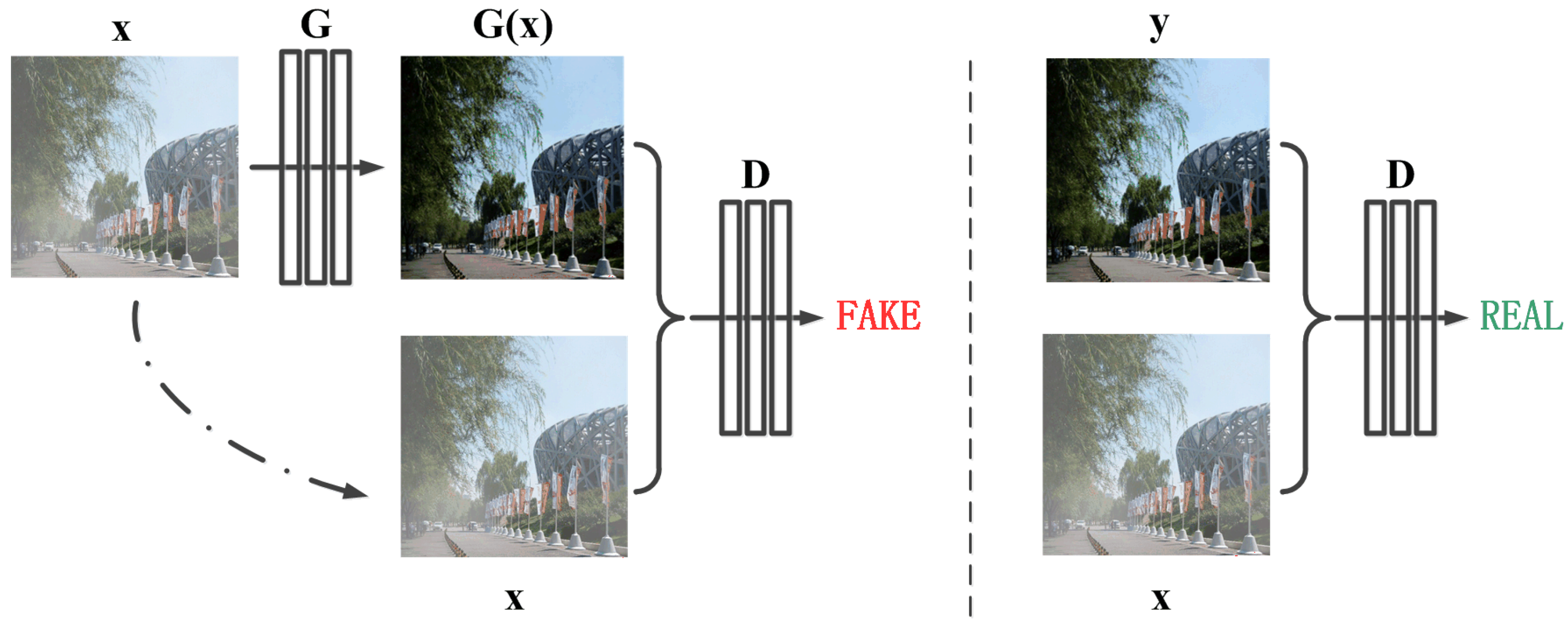
Figure 1.
The architecture of the proposed framework. “G” denotes the generator and “D” denotes the discriminator. “x” is the input hazy image, “G(x)” is the reconstructed hazy-free image and “y” is the clear image. Unlike the unconditional GAN framework, both the generator and discriminator observe the input hazy image.
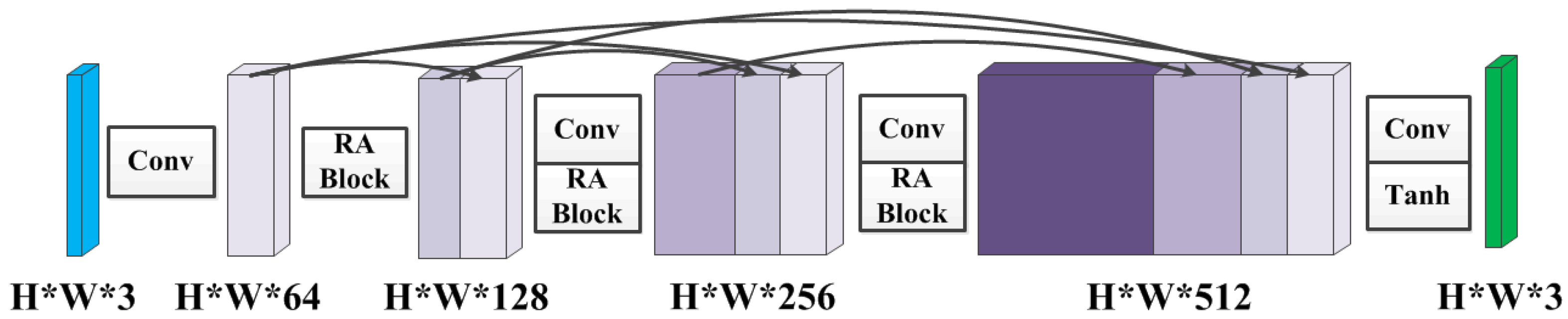
Figure 2.
The densely connected structure as the generator. Each “Conv” contains sequence Conv-BN-ReLU, “Tanh” contains sequence Conv-Tanh, and “RA Block” refers to the residual spatial and channel attention module. “Conv” denotes the convolution, “BN” denotes the batch normalization, “ReLU” denotes the rectified linear unit, and “Tanh” denotes an hyperbolic tangent function. The kernel size of each convolution operation is , the stride is , and the padding is . The input and output channel numbers can be obtained according to the parameters in the figure.
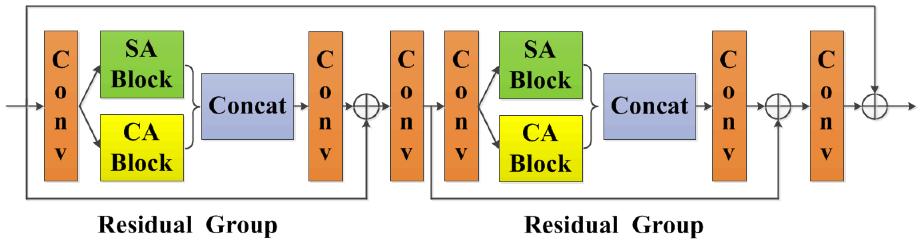
Figure 3.
The residual spatial and channel attention module. Each “Conv” contains sequence Conv-BN-ReLU, “SA Block” refers to spatial attention block, and “CA Block” refers to channel attention block, “Concat” refers to concatenation. The kernel size of each convolution operation is , the stride is , and the padding is . Let C represent the channel number of the input feature maps, then the input and output channel numbers of 1st, 3rd, 4th and 6th convolution operations are C, and the input and output channel numbers of 2nd and 5th convolution operations are and C, respectively.
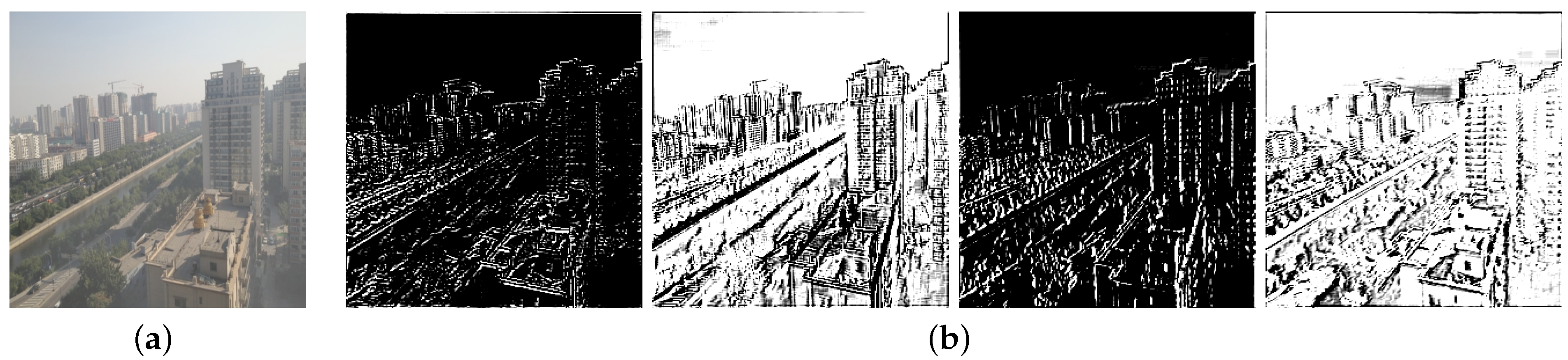
Figure 4.
Samples of feature maps: (a) input image; (b) feature maps extracted from (a).
Figure 4.
Samples of feature maps: (a) input image; (b) feature maps extracted from (a).
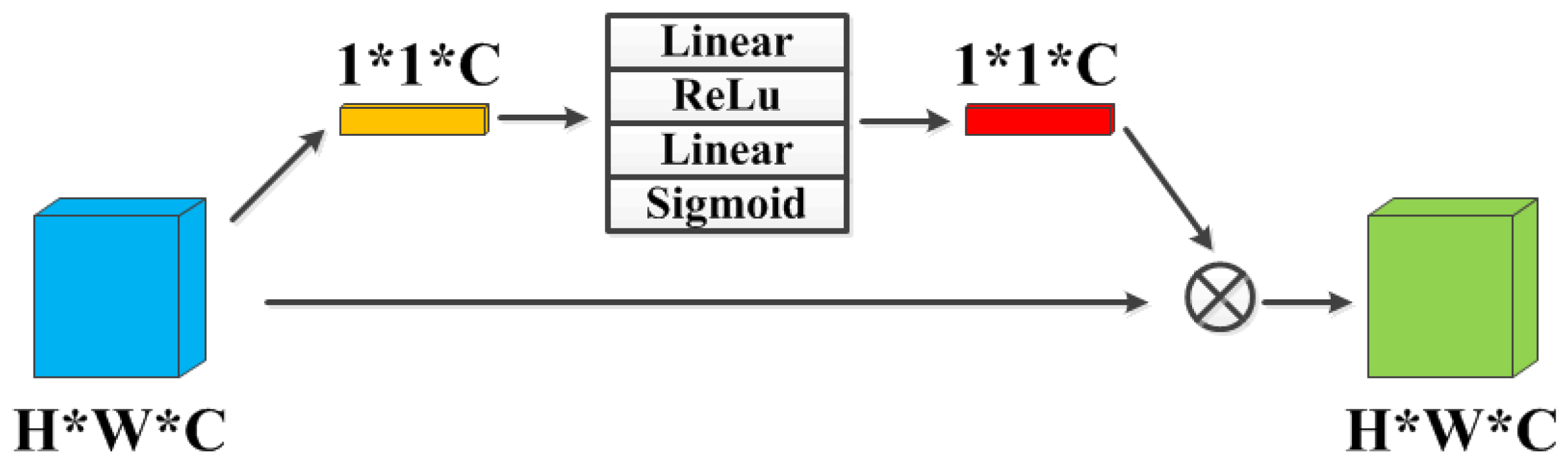
Figure 5.
CA Block: The channel attention module. “Linear” and “Sigmoid” denote the linear and sigmoid function, respectively.
Figure 5.
CA Block: The channel attention module. “Linear” and “Sigmoid” denote the linear and sigmoid function, respectively.
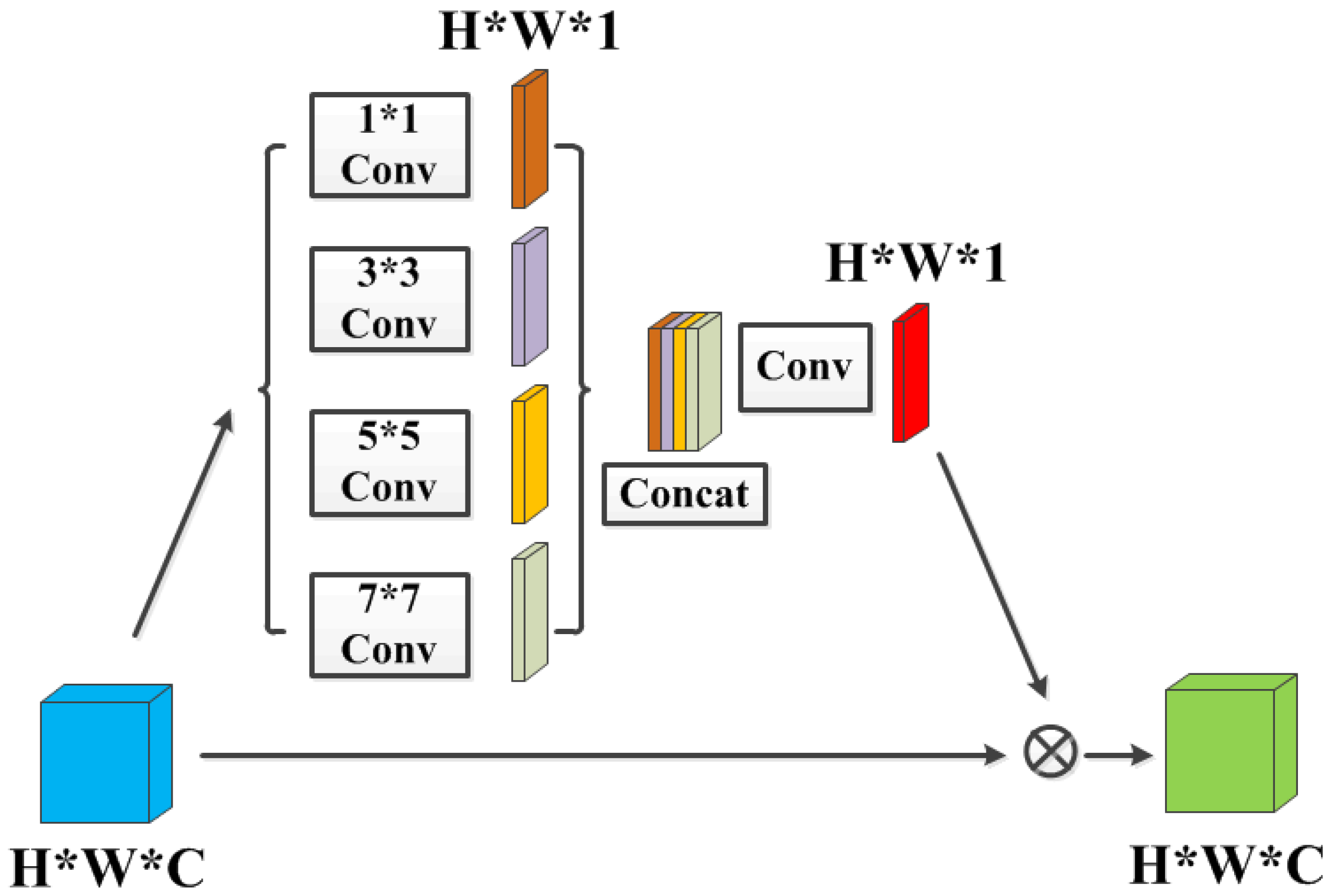
Figure 6.
SA Block: The spatial attention module. Each “Conv” contains sequence Conv-BN-ReLU, “Concat” refers to concatenation. The kernel size of the last convolution operation is , the stride is , and the padding is . The input and output channel numbers are 4 and 1, respectively.
Figure 6.
SA Block: The spatial attention module. Each “Conv” contains sequence Conv-BN-ReLU, “Concat” refers to concatenation. The kernel size of the last convolution operation is , the stride is , and the padding is . The input and output channel numbers are 4 and 1, respectively.
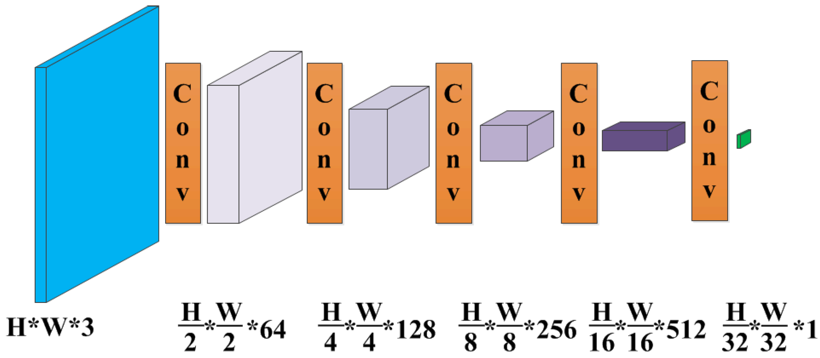
Figure 7.
The PatchGAN architecture as the discriminator. Each “Conv” contains sequence Conv-BN-ReLU. The kernel size of each convolution operation is , the stride is , and the padding is . The input and output channel numbers can be obtained according to the parameters in the figure.
Figure 7.
The PatchGAN architecture as the discriminator. Each “Conv” contains sequence Conv-BN-ReLU. The kernel size of each convolution operation is , the stride is , and the padding is . The input and output channel numbers can be obtained according to the parameters in the figure.
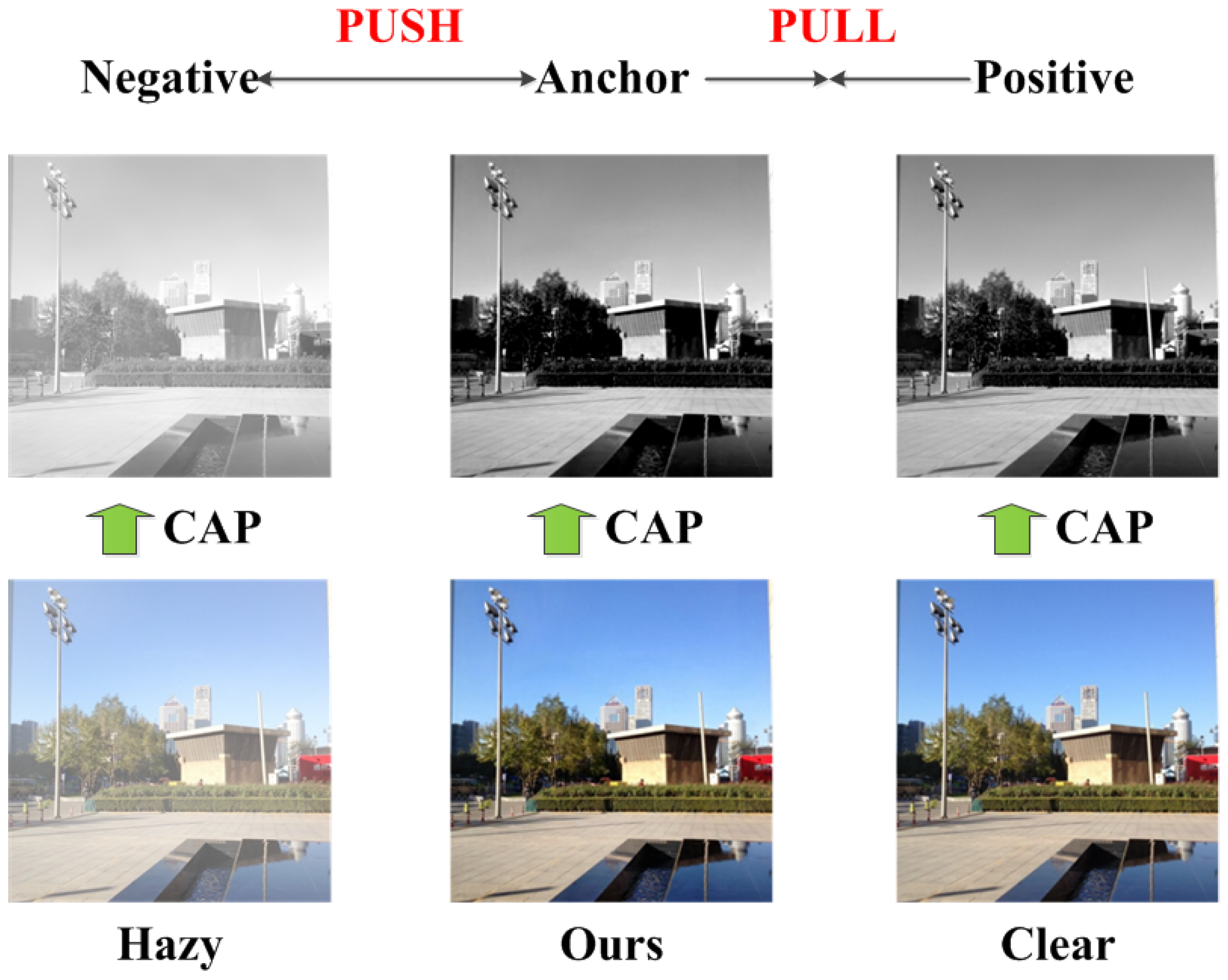
Figure 8.
The diagram of contrastive learning. “CAP” denotes the process of obtaining concentration of haze based on color attenuation prior.
Figure 8.
The diagram of contrastive learning. “CAP” denotes the process of obtaining concentration of haze based on color attenuation prior.
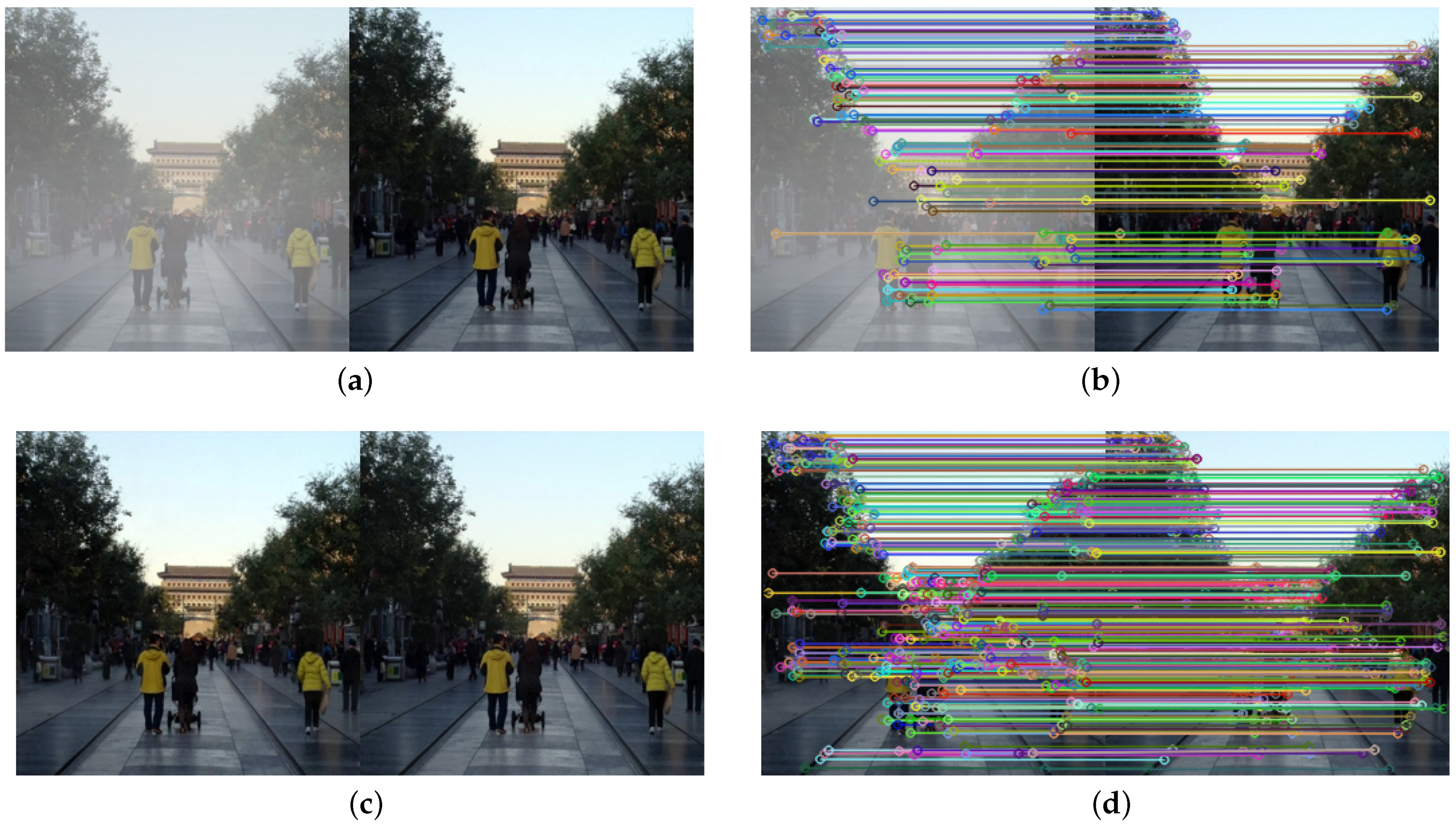
Figure 9.
The schematic diagram of image registration: (a) the hazy and corresponding haze-free images; (b) image registration of (a); (c) the restored and corresponding haze-free images; (d) image registration of (c).
Figure 9.
The schematic diagram of image registration: (a) the hazy and corresponding haze-free images; (b) image registration of (a); (c) the restored and corresponding haze-free images; (d) image registration of (c).
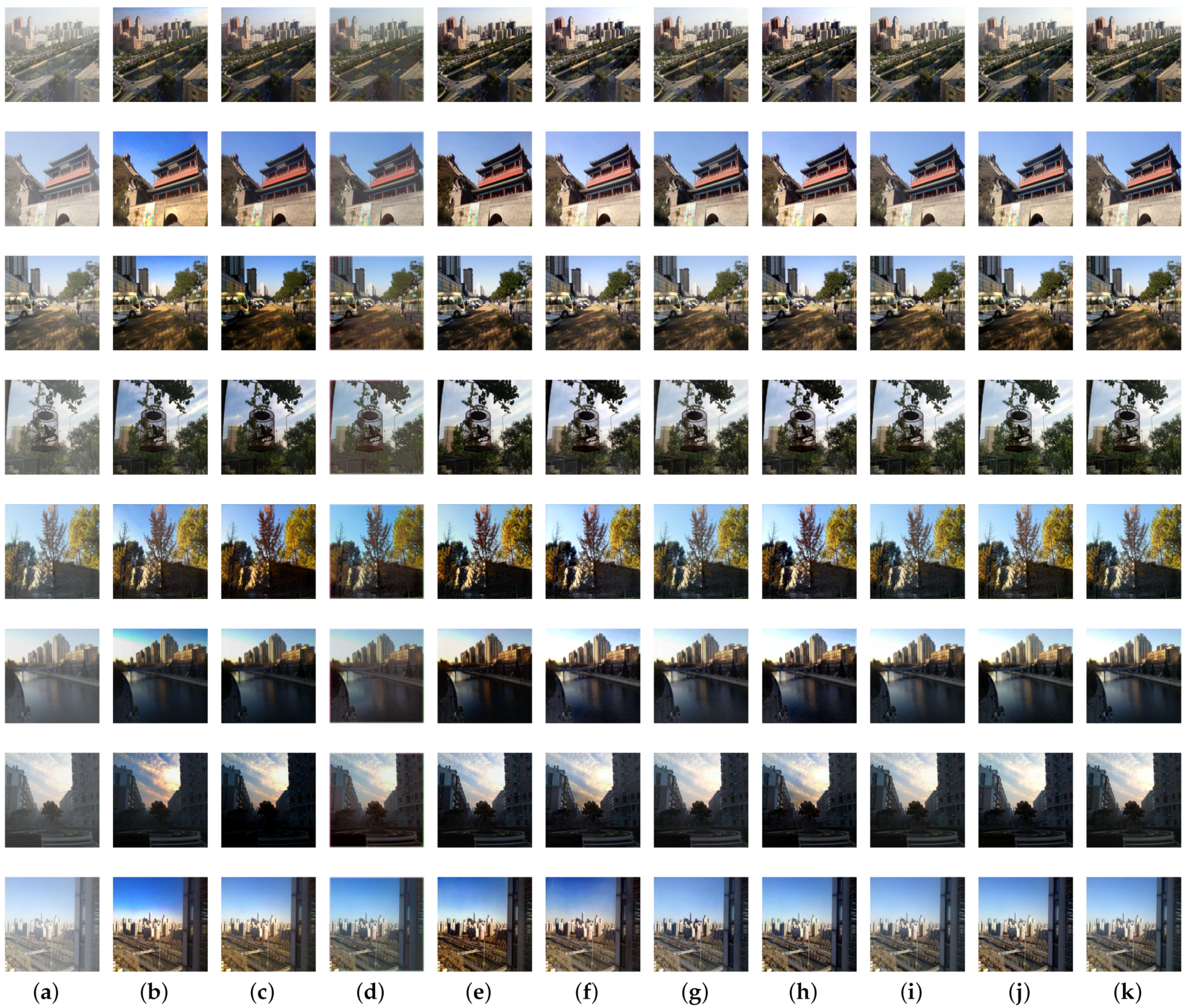
Figure 10.
Visual results on synthetic images of RESIDE dataset: (a) hazy images; (b) DCP; (c) CAP; (d) AODNet; (e) EPDN; (f) GCANet; (g) pix2pix; (h) FFA-Net; (i) Two-branch; (j) our proposed method; (k) corresponding haze-free images.
Figure 10.
Visual results on synthetic images of RESIDE dataset: (a) hazy images; (b) DCP; (c) CAP; (d) AODNet; (e) EPDN; (f) GCANet; (g) pix2pix; (h) FFA-Net; (i) Two-branch; (j) our proposed method; (k) corresponding haze-free images.
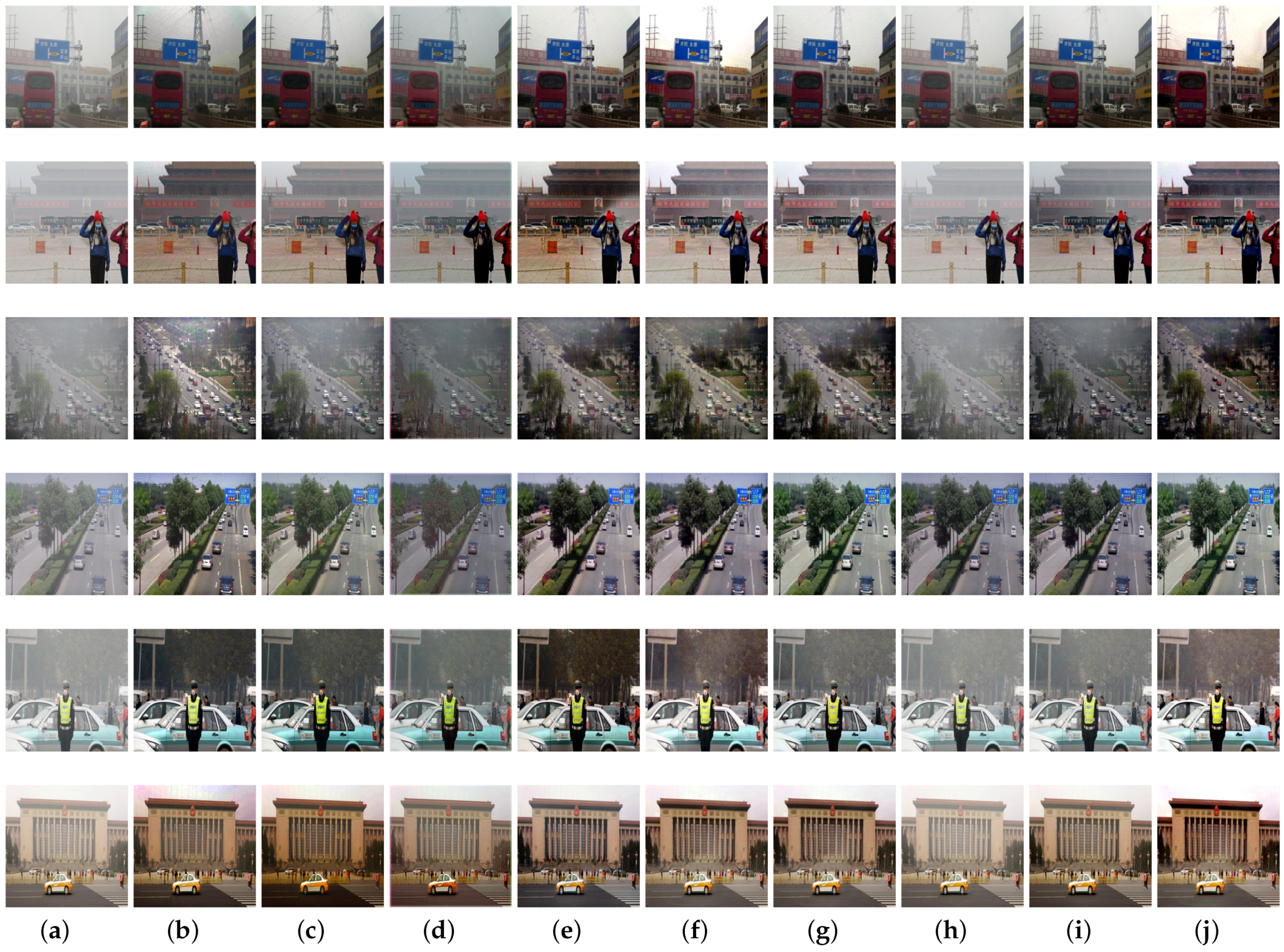
Figure 11.
Visual comparisons on real-world images. (a) Hazy images. (b) DCP. (c) CAP. (d) AODNet. (e) EPDN. (f) GCANet. (g) pix2pix. (h) FFA-Net. (i) Two-branch. (j) Our proposed method.
Figure 11.
Visual comparisons on real-world images. (a) Hazy images. (b) DCP. (c) CAP. (d) AODNet. (e) EPDN. (f) GCANet. (g) pix2pix. (h) FFA-Net. (i) Two-branch. (j) Our proposed method.
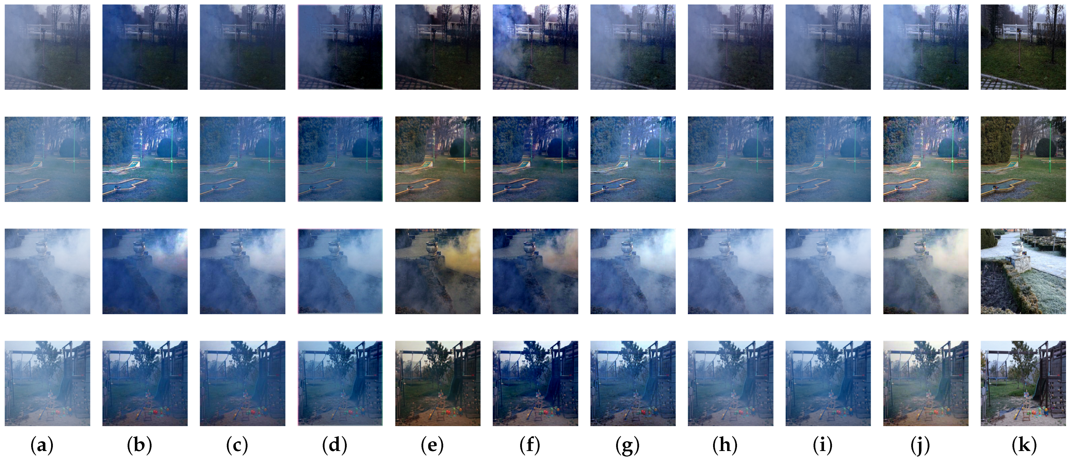
Figure 12.
Visual comparisons on the NTIRE dehazing challenge datasets: (a) hazy images; (b) DCP; (c) CAP; (d) AODNet; (e) EPDN; (f) GCANet; (g) pix2pix; (h) FFA-Net; (i) two-branch; (j) our proposed method; (k) corresponding haze-free images.
Figure 12.
Visual comparisons on the NTIRE dehazing challenge datasets: (a) hazy images; (b) DCP; (c) CAP; (d) AODNet; (e) EPDN; (f) GCANet; (g) pix2pix; (h) FFA-Net; (i) two-branch; (j) our proposed method; (k) corresponding haze-free images.
Figure 13.
Visual results on the NTIRE dehazing challenge datasets with the network training on RESIDE datasets: (a) hazy images; (b) DCP; (c) CAP; (d) AODNet; (e) EPDN; (f) GCANet; (g) pix2pix; (h) FFA-Net; (i) two-branch; (j) our proposed method; (k) corresponding haze-free images.
Figure 13.
Visual results on the NTIRE dehazing challenge datasets with the network training on RESIDE datasets: (a) hazy images; (b) DCP; (c) CAP; (d) AODNet; (e) EPDN; (f) GCANet; (g) pix2pix; (h) FFA-Net; (i) two-branch; (j) our proposed method; (k) corresponding haze-free images.
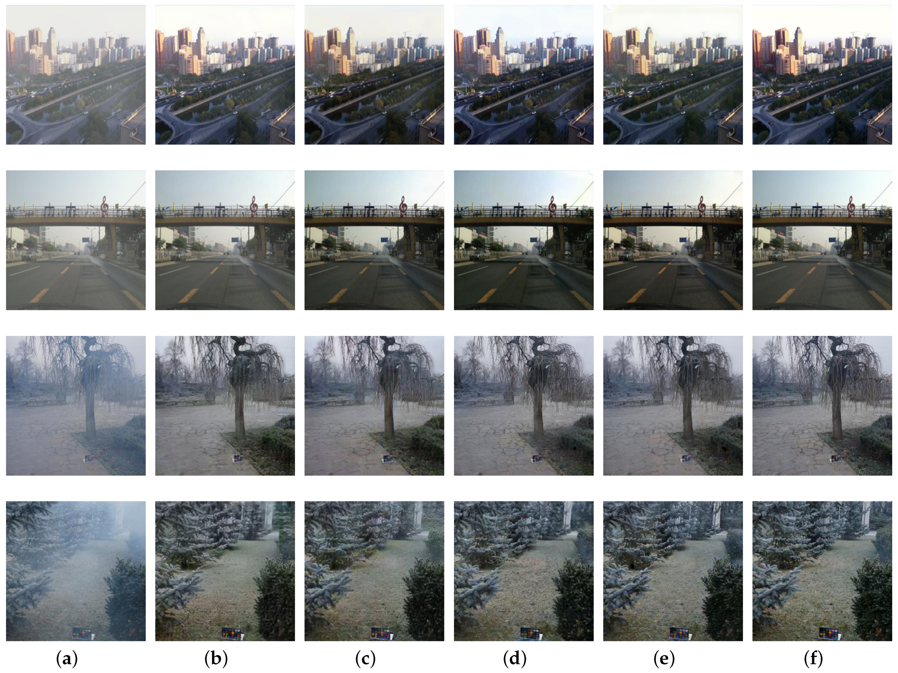
Figure 14.
Visual comparisons with different attention modules: (a) hazy images; (b) RG; (c) RG+CA; (d) RG+SA; (e) RG+CA+SA; (f) corresponding haze-free images.
Figure 14.
Visual comparisons with different attention modules: (a) hazy images; (b) RG; (c) RG+CA; (d) RG+SA; (e) RG+CA+SA; (f) corresponding haze-free images.
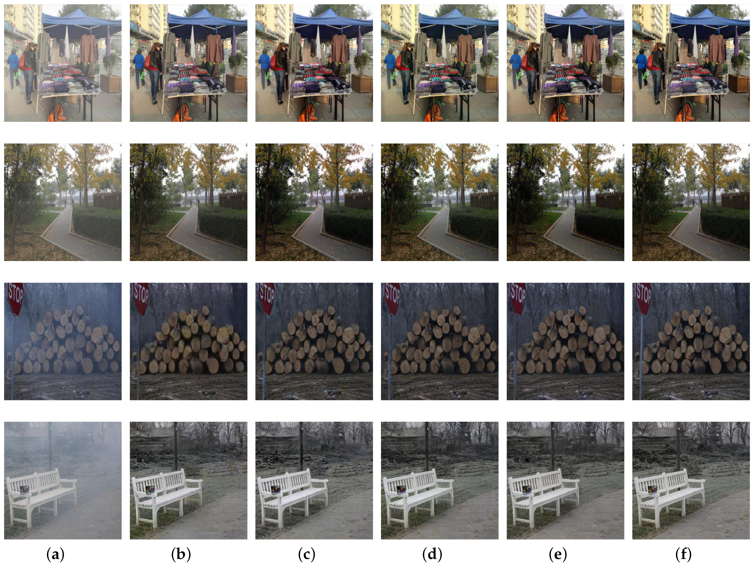
Figure 15.
Visual results with different loss functions: (a) hazy images; (b) without both losses; (c) without registration loss; (d) without contrastive loss; (e) with both losses; (f) corresponding haze-free images.
Figure 15.
Visual results with different loss functions: (a) hazy images; (b) without both losses; (c) without registration loss; (d) without contrastive loss; (e) with both losses; (f) corresponding haze-free images.
Table 1.
Quantitative comparisons with other methods on synthetic images.
Table 1.
Quantitative comparisons with other methods on synthetic images.
| Metrics | DCP | CAP | AODNet | EPDN | GCANet | pix2pix | FFA-Net | Two-Branch | Ours |
|---|
| PSNR | 17.4582 | 18.3581 | 19.7542 | 21.3050 | 23.4265 | 26.9524 | 31.0752 | 32.8842 | 32.9660 |
| SSIM | 0.8752 | 0.8102 | 0.8697 | 0.8793 | 0.9124 | 0.9283 | 0.9548 | 0.9680 | 0.9683 |
| PI | 2.7793 | 2.9076 | 3.0314 | 2.8232 | 2.8774 | 2.7966 | 2.7861 | 2.7912 | 2.7927 |
Table 2.
Quantitative results on the NTIRE dehazing challenge datasets.
Table 2.
Quantitative results on the NTIRE dehazing challenge datasets.
| Metrics | DCP | CAP | AODNet | EPDN | GCANet | pix2pix | FFA-Net | Two-Branch | Ours |
|---|
| PSNR | 17.9749 | 17.0929 | 17.1099 | 17.1335 | 17.9412 | 18.4239 | 17.6025 | 19.5301 | 19.2072 |
| SSIM | 0.6958 | 0.6546 | 0.6174 | 0.7013 | 0.7258 | 0.7334 | 0.6890 | 0.7624 | 0.7454 |
| PI | 2.9803 | 3.4075 | 3.5217 | 2.8029 | 2.8139 | 2.7451 | 3.2858 | 2.8142 | 2.7874 |
Table 3.
Quantitative comparisons on the NTIRE dehazing challenge datasets with the network training on RESIDE datasets.
Table 3.
Quantitative comparisons on the NTIRE dehazing challenge datasets with the network training on RESIDE datasets.
| Metrics | DCP | CAP | AODNet | EPDN | GCANet | pix2pix | FFA-Net | Two-Branch | Ours |
|---|
| PSNR | 13.0425 | 12.6594 | 12.6873 | 13.3428 | 13.4772 | 13.1627 | 12.7565 | 12.7378 | 13.6301 |
| SSIM | 0.5162 | 0.4828 | 0.5047 | 0.5583 | 0.5669 | 0.5311 | 0.5343 | 0.5427 | 0.5896 |
| PI | 4.3941 | 5.2311 | 5.3762 | 4.3171 | 3.9761 | 4.5535 | 5.2122 | 5.8446 | 4.4889 |
Table 4.
Quantitative comparisons with different attention module on RESIDE dataset.
Table 4.
Quantitative comparisons with different attention module on RESIDE dataset.
| Metrics | RG | RG+CA | RG+SA | RG+CA+SA |
|---|
| PSNR | 28.9251 | 31.1037 | 31.3245 | 32.9660 |
| SSIM | 0.9328 | 0.9523 | 0.9583 | 0.9683 |
| PI | 2.7469 | 2.8667 | 2.7142 | 2.7927 |
Table 5.
Quantitative results with different attention module on NTIRE dehazing challenge datasets.
Table 5.
Quantitative results with different attention module on NTIRE dehazing challenge datasets.
| Metrics | RG | RG+CA | RG+SA | RG+CA+SA |
|---|
| PSNR | 18.1372 | 18.5522 | 18.8035 | 19.2072 |
| SSIM | 0.7228 | 0.7366 | 0.7262 | 0.7454 |
| PI | 2.6952 | 2.7913 | 2.7795 | 2.7874 |
Table 6.
Quantitative results with different loss functions on RESIDE dataset. ’wob’, ’wor’, ’woc’ and ’wb’ denote without both losses, without registration loss, without contrastive loss and with both losses, respectively.
Table 6.
Quantitative results with different loss functions on RESIDE dataset. ’wob’, ’wor’, ’woc’ and ’wb’ denote without both losses, without registration loss, without contrastive loss and with both losses, respectively.
| Metrics | Wob | Wor | Woc | Wb |
|---|
| PSNR | 30.3453 | 32.0425 | 31.9728 | 32.9660 |
| SSIM | 0.9482 | 0.9581 | 0.9561 | 0.9683 |
| PI | 2.7825 | 2.8143 | 2.7682 | 2.7927 |
Table 7.
Quantitative comparisons with different loss functions on NTIRE dehazing challenge datasets. ’wob’, ’wor’, ’woc’ and ’wb’ denote without both losses, without registration loss, without contrastive loss and with both losses, respectively.
Table 7.
Quantitative comparisons with different loss functions on NTIRE dehazing challenge datasets. ’wob’, ’wor’, ’woc’ and ’wb’ denote without both losses, without registration loss, without contrastive loss and with both losses, respectively.
| Metrics | Wob | Wor | Woc | Wb |
|---|
| PSNR | 18.6476 | 18.9427 | 18.8752 | 19.2072 |
| SSIM | 0.7392 | 0.7424 | 0.7416 | 0.7454 |
| PI | 2.7351 | 2.7477 | 2.7895 | 2.7874 |


