
Path Planning Generator with Metadata through a Domain Change by GAN between Physical and Virtual Environments


Abstract
:1. Introduction
2. Background and Research Gaps
GAN Cost Functions
3. Proposed Work
3.1. Domain Connection by GAN Approach
3.2. Path Planner Generator with Metadata
3.3. Metadata Information for Each Node
| Algorithm 1 Algorithm to describe path planning’s features. |
| Input: set of 500 virtual samples. Output: path’s description with virtual elements. Initialization:
|
| Algorithm 2 Algorithm for generating dataset. |
| Input: Define the behavior of each obstacles in the environment. Output: set of estimated path. Initialization:
|
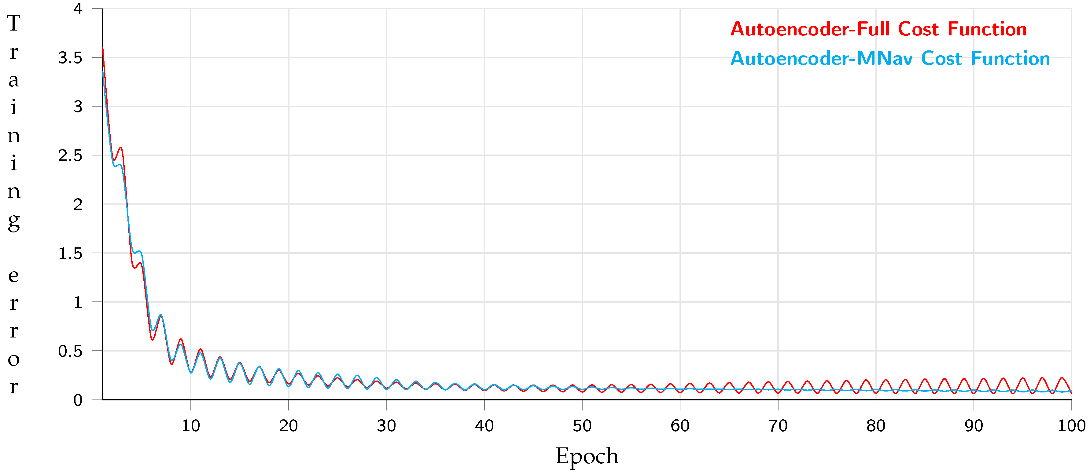
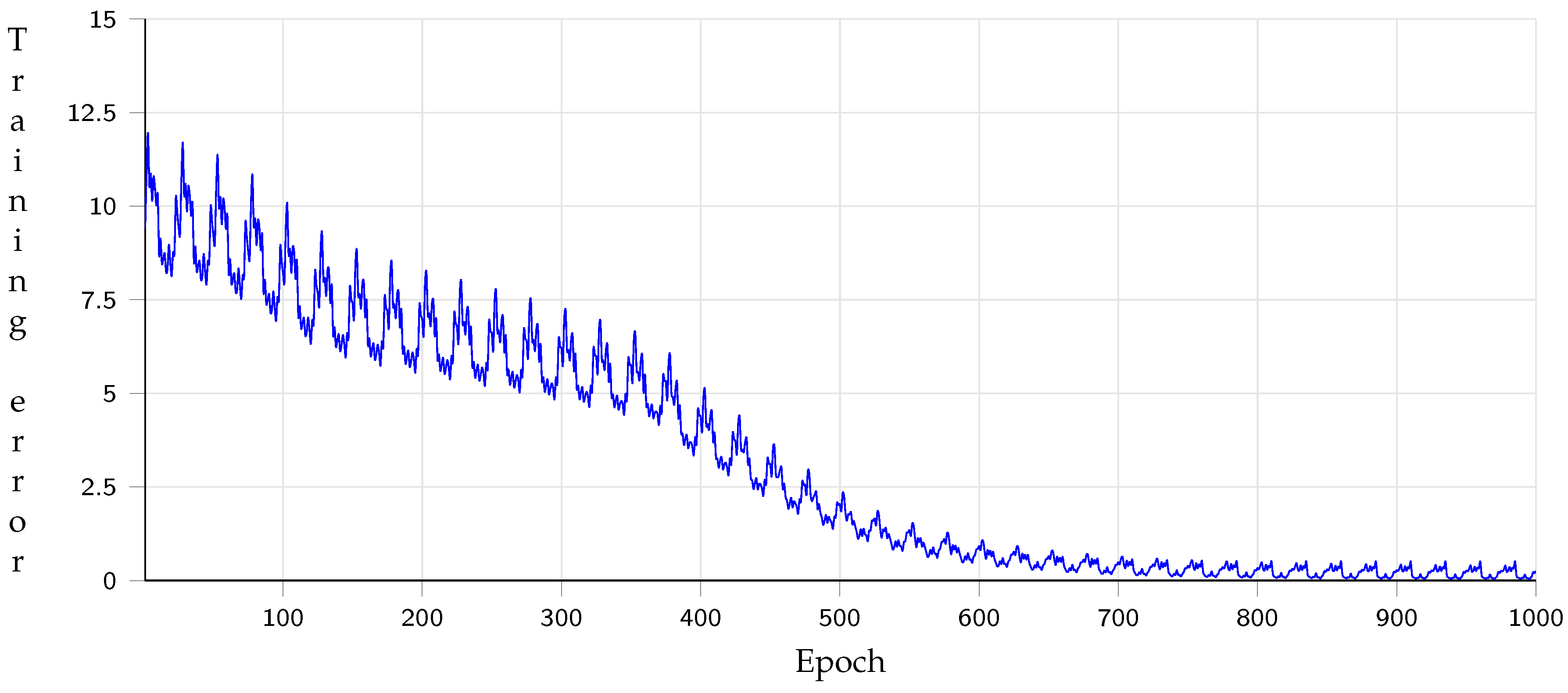
3.4. End-to-End Approach Using an Auto-Encoder
4. Implementation into a Controlled Real Environment
4.1. Interoperability Coefficient Composed by Image Quality and Join Entropy
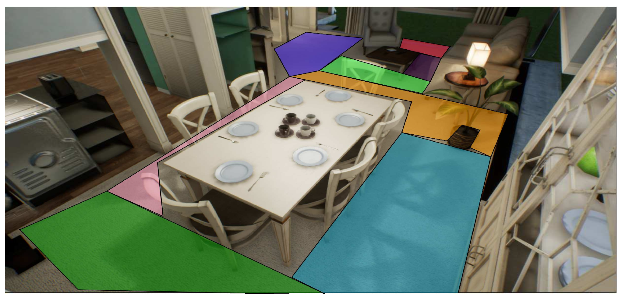
4.2. Virtual Dataset
5. Experimental Results and Analysis
5.1. Path Planning Generator with Metadata Performance
5.2. Interoperability Performance
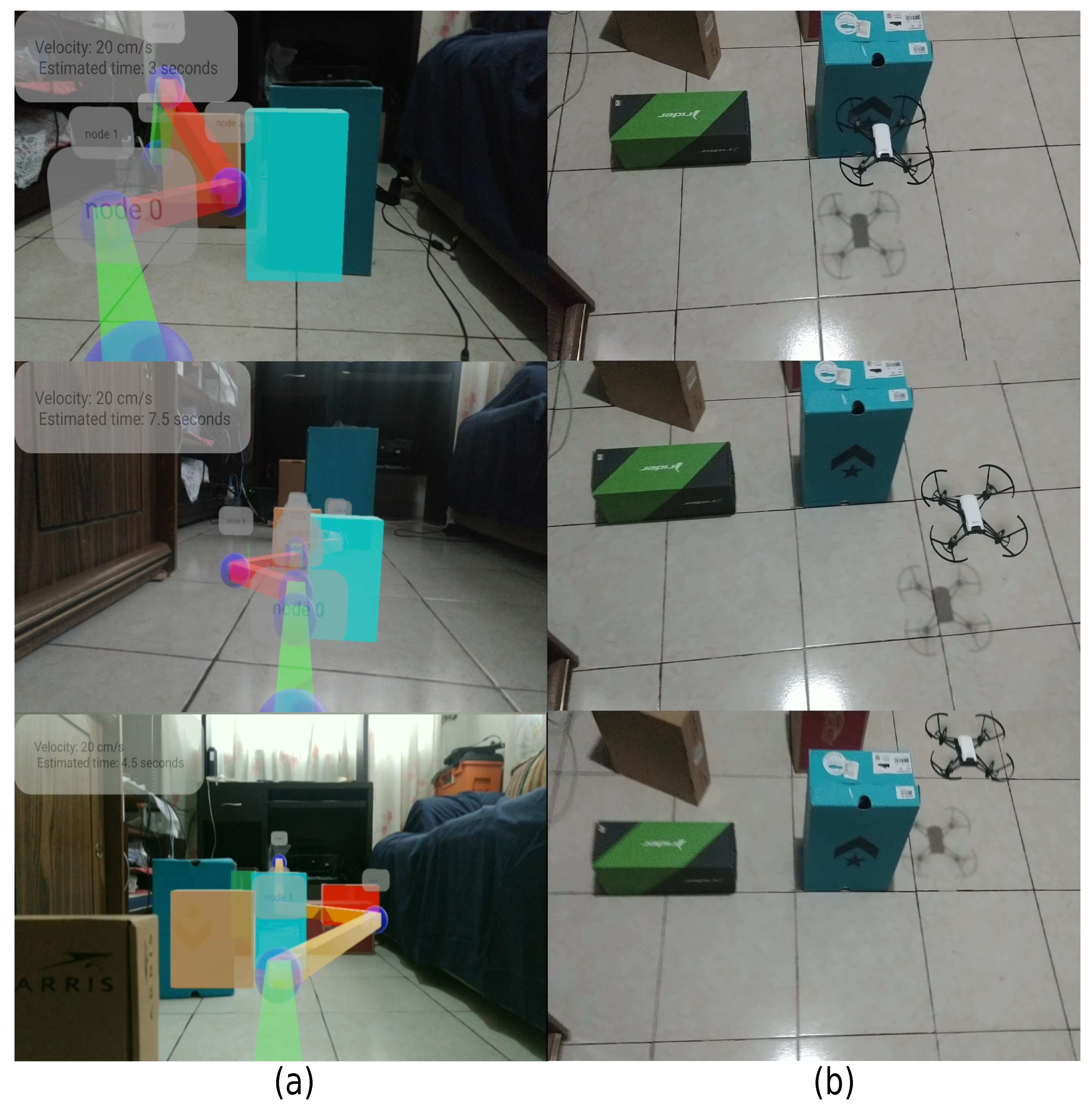
5.3. Performance through an Augmented Reality System and a Real MAV
6. Conclusions
Author Contributions
Funding
Institutional Review Board Statement
Informed Consent Statement
Data Availability Statement
Acknowledgments
Conflicts of Interest
References
- Tian, Y.; Chen, X.; Xiong, H.; Li, H.; Dai, L.; Chen, J.; Xing, J.; Chen, J.; Wu, X.; Hu, W.; et al. Towards human-like and transhuman perception in AI 2.0: A review. Front. Inf. Technol. Electron. Eng. 2017, 18, 58–67. [Google Scholar] [CrossRef]
- Romeo, L.; Petitti, A.; Marani, R.; Milella, A. Internet of Robotic Things in Smart Domains: Applications and Challenges. Sensors 2020, 20, 3355. [Google Scholar] [CrossRef]
- Lighthill, I. Artificial Intelligence: A General Survey. In Artificial Intelligence: A Paper Symposium; Science Research Council: London, UK, 1973. [Google Scholar]
- Pendleton, S.D.; Andersen, H.; Du, X.; Shen, X.; Meghjani, M.; Eng, Y.H.; Rus, D.; Ang, M.H. Perception, Planning, Control, and Coordination for Autonomous Vehicles. Machines 2017, 5, 6. [Google Scholar] [CrossRef]
- Schwartz, J.T.; Sharir, M. On the piano movers’ problem: II. General techniques for computing topological properties of real algebraic manifolds. Adv. Appl. Math. 1983, 4, 298351. [Google Scholar] [CrossRef] [Green Version]
- Chen, L.; Wang, Q.; Lu, X.; Cao, D.; Wang, F. Learning Driving Models From Parallel End-to-End Driving Data Set. Proc. IEEE 2020, 108, 262–273. [Google Scholar] [CrossRef]
- Weiss, K.; Khoshgoftaar, T.M.; Wang, D. A survey of transfer learning. J. Big Data 2016, 3, 9. [Google Scholar] [CrossRef] [Green Version]
- Yoh, M.S. The reality of virtual reality. In Proceedings of the Seventh International Conference on Virtual Systems and Multimedia, Berkeley, CA, USA, 25–27 October 2001; pp. 666–674. [Google Scholar] [CrossRef]
- Oh, I.; Rho, S.; Moon, S.; Son, S.; Lee, H.; Chung, J. Creating Pro-Level AI for a Real-Time Fighting Game Using Deep Reinforcement Learning. IEEE Trans. Games 2021. [Google Scholar] [CrossRef]
- Aggarwal, R.; Singhal, A. Augmented Reality and its effect on our life. In Proceedings of the 2019 9th International Conference on Cloud Computing, Data Science & Engineering (Confluence), Noida, India, 10–11 January 2019; pp. 510–515. [Google Scholar] [CrossRef]
- Maldonado-Romo, J.; Aldape-Pérez, M. Interoperability between Real and Virtual Environments Connected by a GAN for the Path-Planning Problem. Appl. Sci. 2021, 11, 10445. [Google Scholar] [CrossRef]
- Yu, L.; Zhang, W.; Wang, J.; Yu, Y. SeqGAN: Sequence generative adversarial nets with policy gradient. In Proceedings of the AAAI Conference on Artificial Intelligence, San Francisco, CA, USA, 4–9 February 2017; pp. 2852–2858. [Google Scholar]
- Siegwart, R.; Nourbakhsh, I.R.; Scaramuzza, D. Introduction to Autonomous Mobile Robots; The Mit Press: London, UK, 1997. [Google Scholar]
- Si, J.; Yang, L.; Lu, C.; Sun, J.; Mei, S. Approximate dynamic programming for continuous state and control problems. In Proceedings of the 2009 17th Mediterranean Conference on Control and Automation, Thessaloniki, Greece, 24–26 June 2009; pp. 1415–1420. [Google Scholar] [CrossRef]
- Jiao, J.; Liu, S.; Deng, H.; Lai, Y.; Li, F.; Mei, T.; Huang, H. Design and Fabrication of Long Soft-Robotic Elastomeric Actuator Inspired by Octopus Arm. In Proceedings of the 2019 IEEE International Conference on Robotics and Biomimetics (ROBIO), Dali, China, 6–8 December 2019; pp. 2826–2832. [Google Scholar] [CrossRef]
- Spiteri, R.J.; Ascher, U.M.; Pai, D.K. Numerical solution of differential systems with algebraic inequalities arising in robot programming. In Proceedings of the 1995 IEEE International Conference on Robotics and Automation, Nagoya, Japan, 21–27 May 1995; Volume 3, pp. 2373–2380. [Google Scholar] [CrossRef]
- Karaman, S.; Frazzoli, E. Incremental sampling-based algorithms for optimal motion planning. arXiv 2010, arXiv:1005.0416. [Google Scholar]
- Musliman, I.A.; Rahman, A.A.; Coors, V. Implementing 3D network analysis in 3D-GIS. Int. Arch. ISPRS 2008, 37. Available online: https://citeseerx.ist.psu.edu/viewdoc/download?doi=10.1.1.640.7225&rep=rep1&type=pdf (accessed on 15 November 2021).
- Pehlivanoglu, Y.V.; Baysal, O.; Hacioglu, A. Path planning for autonomous UAV via vibrational genetic algorithm. Aircr. Eng. Aerosp. Technol. Int. J. 2007, 79, 352–359. [Google Scholar] [CrossRef]
- Yan, F.; Liu, Y.S.; Xiao, J.Z. Path planning in complex 3D environments using a probabilistic roadmap method. Int. J. Autom. Comput. 2013, 10, 525–533. [Google Scholar] [CrossRef]
- Mittal, P.; Singh, R.; Sharma, A. Deep learning-based object detection in low-altitude UAV datasets: A survey. Image Vis. Comput. 2020, 104, 104046. [Google Scholar] [CrossRef]
- Alam, M.S.; Oluoch, J. A survey of safe landing zone detection techniques for autonomous unmanned aerial vehicles (UAVs). Expert Syst. Appl. 2021, 179, 115091. [Google Scholar] [CrossRef]
- Khuc, T.; Nguyen, T.A.; Dao, H.; Catbas, F.N. Swaying displacement measurement for structural monitoring using computer vision and an unmanned aerial vehicle. Measurement 2020, 159, 107769. [Google Scholar] [CrossRef]
- Al-Kaff, A.; Martín, D.; García, F.; Escalera, A.D.; Armingol, J.M. Survey of computer vision algorithms and applications for unmanned aerial vehicles. Expert Syst. Appl. 2018, 92, 447–463. [Google Scholar] [CrossRef]
- Silberman, N.; Hoiem, D.; Kohli, P.; Fergus, R. Indoor Segmentation and Support Inference from RGBD Images. In Computer Vision—ECCV 2012; Lecture Notes in Computer Science; Fitzgibbon, A., Lazebnik, S., Perona, P., Sato, Y., Schmid, C., Eds.; Springer: Berlin/Heidelberg, Germany, 2012; Volume 7576. [Google Scholar] [CrossRef]
- Geiger, A.; Lenz, P.; Stiller, C.; Urtasun, R. Vision meets robotics: The KITTI dataset. Int. J. Rob. Res. 2013, 32, 1231–1237. [Google Scholar] [CrossRef] [Green Version]
- Cordts, M.; Omran, M.; Ramos, S.; Rehfeld, T.; Enzweiler, M.; Benenson, R.; Schiele, B. The Cityscapes Dataset for Semantic Urban Scene Understanding. In Proceedings of the 2016 IEEE Conference on Computer Vision and Pattern Recognition (CVPR), Las Vegas, NV, USA, 27–30 June 2016; pp. 3213–3223. [Google Scholar] [CrossRef] [Green Version]
- Kotsiantis, S.B. RETRACTED ARTICLE: Feature selection for machine learning classification problems: A recent overview. Artif. Intell. Rev. 2011, 42, 157. [Google Scholar] [CrossRef] [Green Version]
- Veena, K.M.; Manjula Shenoy, K.; Ajitha Shenoy, K.B. Performance Comparison of Machine Learning Classification Algorithms. In Communications in Computer and Information Science; Springer: Singapore, 2018; pp. 489–497. [Google Scholar] [CrossRef]
- Wollsen, M.G.; Hallam, J.; Jorgensen, B.N. Novel Automatic Filter-Class Feature Selection for Machine Learning Regression. In Advances in Big Data; Springer: Berlin/Heidelberg, Germany, 2016; pp. 71–80. [Google Scholar] [CrossRef]
- Garcia-Gutierrez, J.; Martínez-Álvarez, F.; Troncoso, A.; Riquelme, J.C. A Comparative Study of Machine Learning Regression Methods on LiDAR Data: A Case Study. In Advances in Intelligent Systems and Computing; Springer: Berlin/Heidelberg, Germany, 2014; pp. 249–258. [Google Scholar] [CrossRef] [Green Version]
- Jebara, T. Machine Learning; Springer: Berlin/Heidelberg, Germany, 2004. [Google Scholar] [CrossRef]
- Karras, T.; Laine, S.; Aila, T. A Style-Based Generator Architecture for Generative Adversarial Networks. In Proceedings of the 2019 IEEE/CVF Conference on Computer Vision and Pattern Recognition (CVPR), Long Beach, CA, USA, 16–20 June 2019; pp. 4396–4405. [Google Scholar] [CrossRef] [Green Version]
- Zhu, J.; Park, T.; Isola, P.; Efros, A.A. Unpaired Image-to-Image Translation Using Cycle-Consistent Adversarial Networks. In Proceedings of the 2017 IEEE International Conference on Computer Vision (ICCV), Venice, Italy, 22–29 October 2017; pp. 2242–2251. [Google Scholar] [CrossRef] [Green Version]
- El-Kaddoury, M.; Mahmoudi, A.; Himmi, M.M. Deep Generative Models for Image Generation: A Practical Comparison Between Variational Autoencoders and Generative Adversarial Networks. In Mobile, Secure, and Programmable Networking; MSPN 2019. Lecture Notes in Computer Science; Renault, É., Boumerdassi, S., Leghris, C., Bouzefrane, S., Eds.; Springer: Cham, Switzerland, 2019; Volume 11557. [Google Scholar] [CrossRef]
- Press, O.; Bar, A.; Bogin, B.; Berant, J.; Wolf, L. Language generation with recurrent generative adversarial networks without pre-training. arXiv 2017, arXiv:1706.01399. [Google Scholar]
- Marinescu, D.C.; Marinescu, G.M. (Eds.) CHAPTER 3—Classical and Quantum Information Theory. In Classical and Quantum Information; Academic Press: Cambridge, MA, USA, 2012; pp. 221–344. ISBN 9780123838742. [Google Scholar] [CrossRef]
- Goodfellow, I.; Pouget-Abadie, J.; Mirza, M.; Xu, B.; Warde-Farley, D.; Ozair, S.; Courville, A.; Bengio, Y. Generative Adversarial Networks. Advances in Neural Information Processing Systems. 2014. Available online: https://proceedings.neurips.cc/paper/2014/file/5ca3e9b122f61f8f06494c97b1afccf3-Paper.pdf (accessed on 15 November 2021).
- Kwak, D.H.; Lee, S.H. A Novel Method for Estimating Monocular Depth Using Cycle GAN and Segmentation. Sensors 2020, 20, 2567. [Google Scholar] [CrossRef]
- Zhang, Z.; Weng, D.; Jiang, H.; Liu, Y.; Wang, Y. Inverse Augmented Reality: A Virtual Agent’s Perspective. In Proceedings of the 2018 IEEE International Symposium on Mixed and Augmented Reality Adjunct (ISMAR-Adjunct), Munich, Germany, 16–20 October 2018; pp. 154–157. [Google Scholar] [CrossRef] [Green Version]
- Lifton, J.; Paradiso, J.A. Dual reality: Merging the real and vir-tual. In International Conference on Facets of Virtual Environments; Springer: Berlin/Heidelberg, Germany, 2009; pp. 12–28. [Google Scholar]
- Roo, J.S.; Hachet, M. One reality: Augmenting how the physical world is experienced by combining multiple mixed reality modalities. In Proceedings of the 30th Annual ACM Symposium on User Interface Software and Technology; ACM: New York, NY, USA, 2017; pp. 787–795. [Google Scholar]
- Shital, S.; Dey, D.; Lovett, C.; Kapoor, A. AirSim: High-Fidelity Visual and Physical Simulation for Autonomous Vehicles. arXiv 2017, arXiv:1705.05065. [Google Scholar]
- Feng, J.; McCurry, C.D.; Zein-Sabatto, S. Design of an integrated environment for operation and control of robotic arms (non-reviewed). In Proceedings of the IEEE SoutheastCon 2008, Huntsville, AL, USA, 3–6 April 2008; p. 295. [Google Scholar] [CrossRef]
- Wang, L. Computational intelligence in autonomous mobile robotics-A review. In Proceedings of the 2002 International Symposium on Micromechatronics and Human Science, Nagoya, Japan, 20–23 October 2002; pp. 227–235. [Google Scholar] [CrossRef]
- Zabarankin, M.; Uryasev, S.; Murphey, R. Aircraft routing under the risk of detection. Nav. Res. Logist. (NRL) 2006, 53, 728–747. [Google Scholar] [CrossRef]
- Xue, Y.; Sun, J.-Q. Solving the Path Planning Problem in Mobile Robotics with the Multi-Objective Evolutionary Algorithm. Appl. Sci. 2018, 8, 1425. [Google Scholar] [CrossRef] [Green Version]
- Huang, Y.; Chen, J.; Ouyang, W.; Wan, W.; Xue, Y. Image Captioning With End-to-End Attribute Detection and Subsequent Attributes Prediction. IEEE Trans. Image Process. 2020, 29, 4013–4026. [Google Scholar] [CrossRef]
- Kajdocsi, L.; Kovács, J.; Pozna, C.R. A great potential for using mesh networks in indoor navigation. In Proceedings of the 2016 IEEE 14th International Symposium on Intelligent Systems and Informatics (SISY), Subotica, Serbia, 29–31 August 2016; pp. 187–192. [Google Scholar] [CrossRef]
- NISO. A Framework of Guidance for Building Good Digital Collections: Metadata. Retrieved, 5 August 2014. 2007. Available online: http://www.niso.org/publications/rp/framework3.pdf (accessed on 25 June 2021).
- Dalal, N.; Triggs, B. Histograms of oriented gradients for human detection. In Proceedings of the 2005 IEEE Computer Society Conference on Computer Vision and Pattern Recognition (CVPR’05), San Diego, CA, USA, 20–25 June 2005; Volume 1, pp. 886–893. [Google Scholar] [CrossRef] [Green Version]
- LeCun, Y.; Bengio, Y.; Hinton, G. Deep learning. Nature 2015, 521, 436–444. [Google Scholar] [CrossRef]
- Jang, B.; Kim, M.; Harerimana, G.; Kim, J.W. Q-Learning Algorithms: A Comprehensive Classification and Applications. IEEE Access 2019, 7, 133653–133667. [Google Scholar] [CrossRef]
- Ceballos, N.D.; Valencia, J.A.; Ospina, N.L.; Barrera, A. Quantitative Performance Metrics for Mobile Robots Navigation; INTECH Open Access Publisher: London, UK, 2010. [Google Scholar] [CrossRef] [Green Version]
- Ibraheem, A.; Peter, W. High Quality Monocular Depth Estimation via Transfer Learning. arXiv 2018, arXiv:1812.11941. [Google Scholar]
- Handa, A. Real-Time Camera Tracking: When is High Frame-Rate Best? In Computer Vision-ECCV 2012; Springer: Berlin/Heidelberg, Germany, 2012; pp. 222–235. [Google Scholar]


| Simple Environment Virtual-Real | Environment with Lights-Materials Virtual-Real | |
|---|---|---|
| Factor Correlation (mean) | 0.3708 | 0.5490 |
| Factor Correlation (std) | 0.0824 | 0.0755 |
| Number of Samples | Join Entropy | Interoperability Coefficient |
|---|---|---|
| 10 | 0.8956 | 0.05731 |
| 20 | 0.6071 | 0.21570 |
| 30 | 0.3075 | 0.38018 |
| 40 | 0.2197 | 0.42384 |
| 50 | 0.1302 | 0.47752 |
| 58 | 0.0887 | 0.50030 |
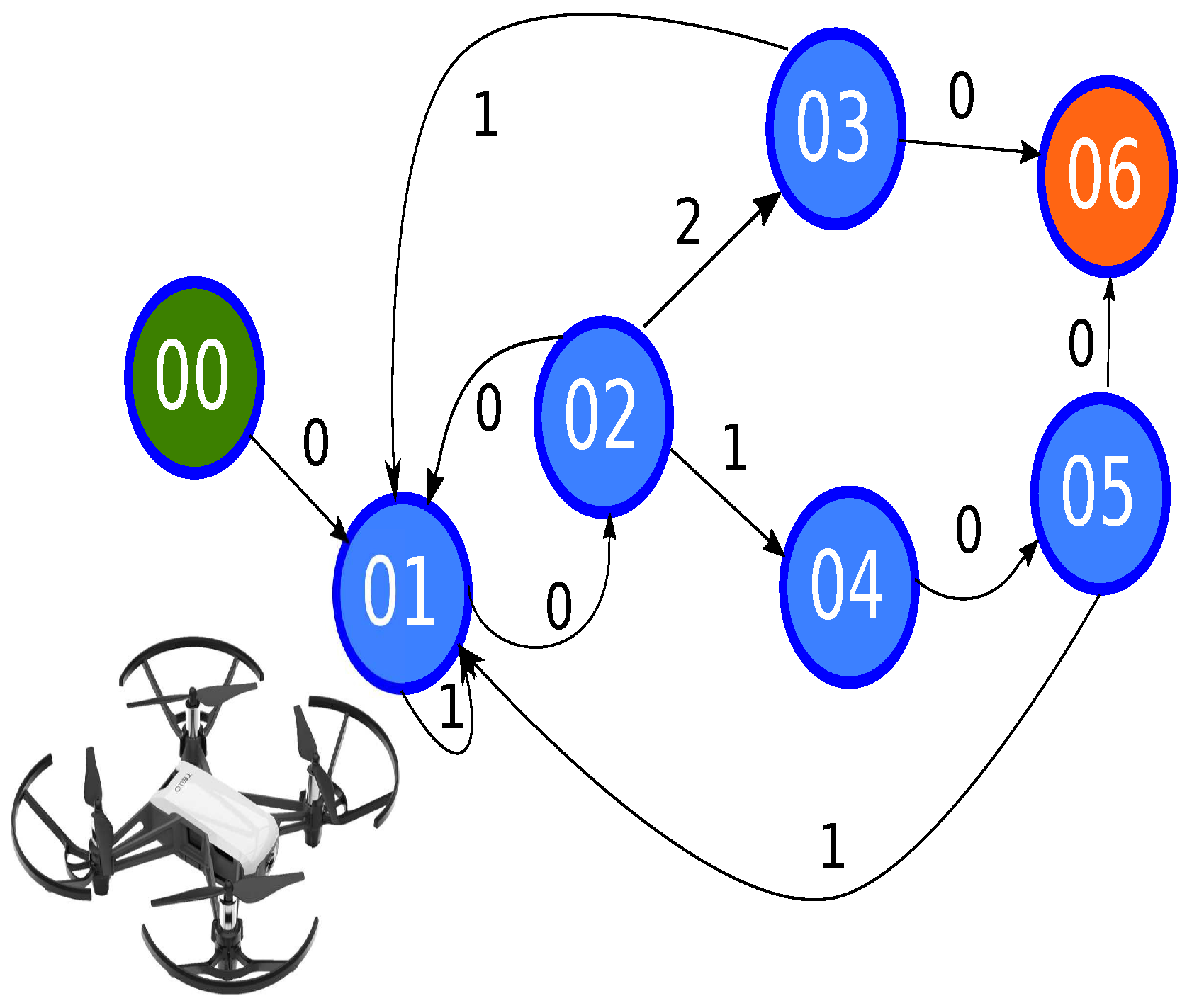
| State | Transition | Description |
|---|---|---|
| 00 | Set the MAV MAV 30 cm above the surface | |
| 01 | Transition 0: get five samples and taking the mean of following movement Transition 1: the response time failed, reset counter | |
| 02 | Transition 0: return to previous state, the movement is randomized Transition 1: diagonal movement Transition 2: the straight movement | |
| 03 | Transition 0: go to final state Transition 1: movement to following node | |
| 04 | Complete the diagonal movement | |
| 05 | Transition 0: go to final state Transition 1: movement to following node | |
| 06 | - | Final state |
| Model | Accuracy Euclidean Distance (Mean-Std) ↓ | Accuracy Manhatan Distance (Mean-Std) ↓ | Accuracy Cosine Similarity (Mean-Std) ↓ | Coefficient Free Collision ↑ |
|---|---|---|---|---|
| AED-MNav-TL | 1.7485 ± 0.2856 | 4.3214 ± 2.1967 | 0.2145 ± 0.0473 | 0.92 |
| Q-learning | 1.5841 ± 0.3658 | 4.8415 ± 1.9927 | 0.1847 ± 0.0308 | 0.96 |
| Feature | Q-Learning | Img2path |
|---|---|---|
| Principal issue | Optimize a policy | Associate a conventional algorithm |
| Training time | Long because of a deep exploration | Short because of a limited exploration |
| Type of environment | Unexplored environments | Known environments |
| Size path | Long because of limited movements | Short because of navigation meshes |
| rel—std ↓ | rms–std ↓ | –std↓ | –std↑ | –std↑ | –std↑ |
|---|---|---|---|---|---|
| 0.8981–0.8452 | 0.9141–0.4889 | 0.4331–0.1245 | 0.6668–0.0202 | 0.8219–0.03458 | 0.8719–0.0318 |
| Model | Accuracy Euclidean Distance (Mean-Std) ↓ | Accuracy Manhatan Distance (Mean-Std) ↓ | Accuracy Cosine Similarity (Mean-Std) ↓ | Coefficient Free Collision ↑ |
|---|---|---|---|---|
| AED-Full | 12.1415 ± 1.0488 | 25.3784 ± 2.2804 | 0.1573 ± 0.0248 | 0.88 |
| AED-MNav | 2.2649 ± 0.4982 | 5.9261 ± 1.9159 | 0.0281 ± 0.0152 | 0.94 |
| AED-Full-TL | 11.7146 ± 1.9251 | 24.8429 ± 1.5279 | 0.1414 ± 0.1097 | 0.86 |
| AED-MNav-TL | 1.7267 ± 0.4194 | 4.7151 ± 1.9014 | 0.0246 ± 0.0204 | 0.94 |
| Device | Float16 (FPS) |
|---|---|
| Jetson nano 2G Tensorflow-lite | 10 |
| Jetson nano 2G Tensor RT | 40 |
| Android device Moto X4 CPU-4 threads | 12 |
| Android device Moto X4 GPU | 18 |
| Android device Moto X4 NN-API | 6 |
| Augmented Reality Free Coefficient | MAV Free Coefficient |
|---|---|
| 0.7666 | 0.5666 |
Publisher’s Note: MDPI stays neutral with regard to jurisdictional claims in published maps and institutional affiliations. |
© 2021 by the authors. Licensee MDPI, Basel, Switzerland. This article is an open access article distributed under the terms and conditions of the Creative Commons Attribution (CC BY) license (https://creativecommons.org/licenses/by/4.0/).
Share and Cite
Maldonado-Romo, J.; Aldape-Pérez, M.; Rodríguez-Molina, A. Path Planning Generator with Metadata through a Domain Change by GAN between Physical and Virtual Environments. Sensors 2021, 21, 7667. https://doi.org/10.3390/s21227667
Maldonado-Romo J, Aldape-Pérez M, Rodríguez-Molina A. Path Planning Generator with Metadata through a Domain Change by GAN between Physical and Virtual Environments. Sensors. 2021; 21(22):7667. https://doi.org/10.3390/s21227667
Chicago/Turabian StyleMaldonado-Romo, Javier, Mario Aldape-Pérez, and Alejandro Rodríguez-Molina. 2021. "Path Planning Generator with Metadata through a Domain Change by GAN between Physical and Virtual Environments" Sensors 21, no. 22: 7667. https://doi.org/10.3390/s21227667
APA StyleMaldonado-Romo, J., Aldape-Pérez, M., & Rodríguez-Molina, A. (2021). Path Planning Generator with Metadata through a Domain Change by GAN between Physical and Virtual Environments. Sensors, 21(22), 7667. https://doi.org/10.3390/s21227667