
An Ensemble Method for Missing Data of Environmental Sensor Considering Univariate and Multivariate Characteristics


Abstract
:1. Introduction
2. Methodology
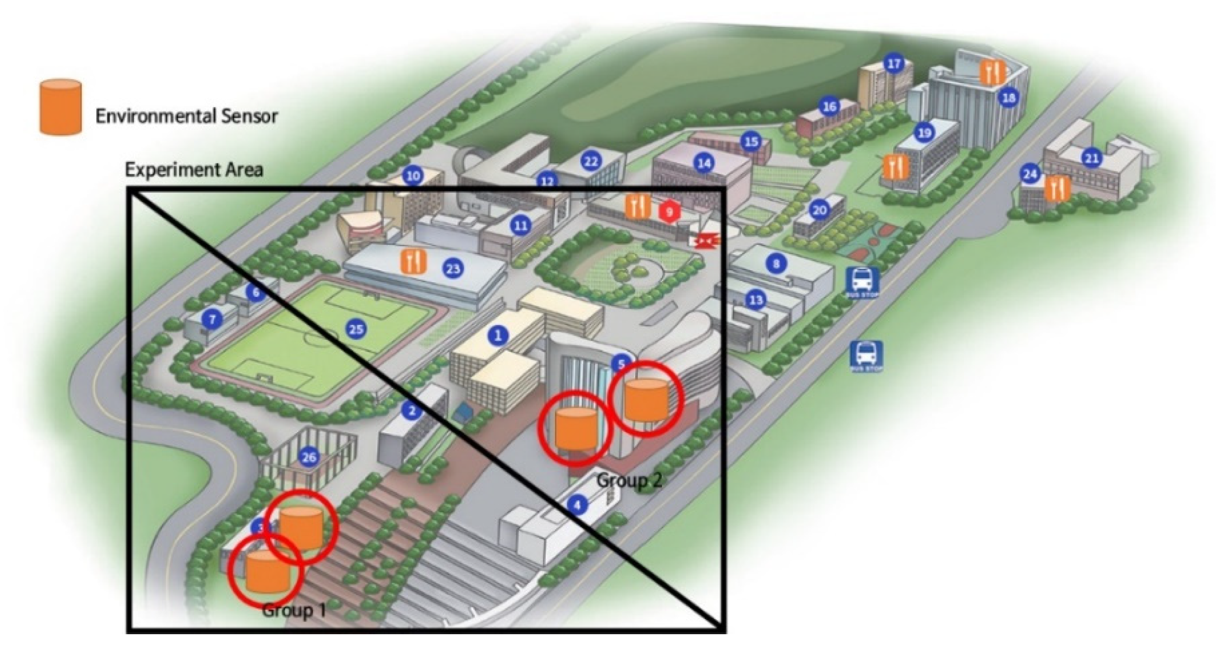
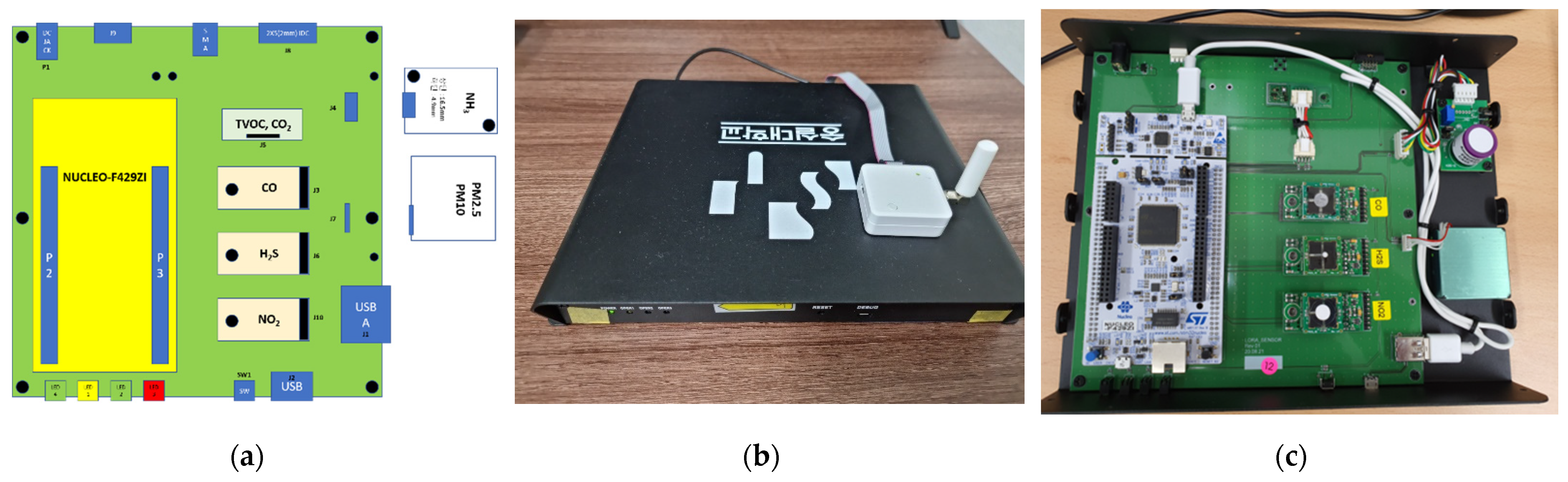
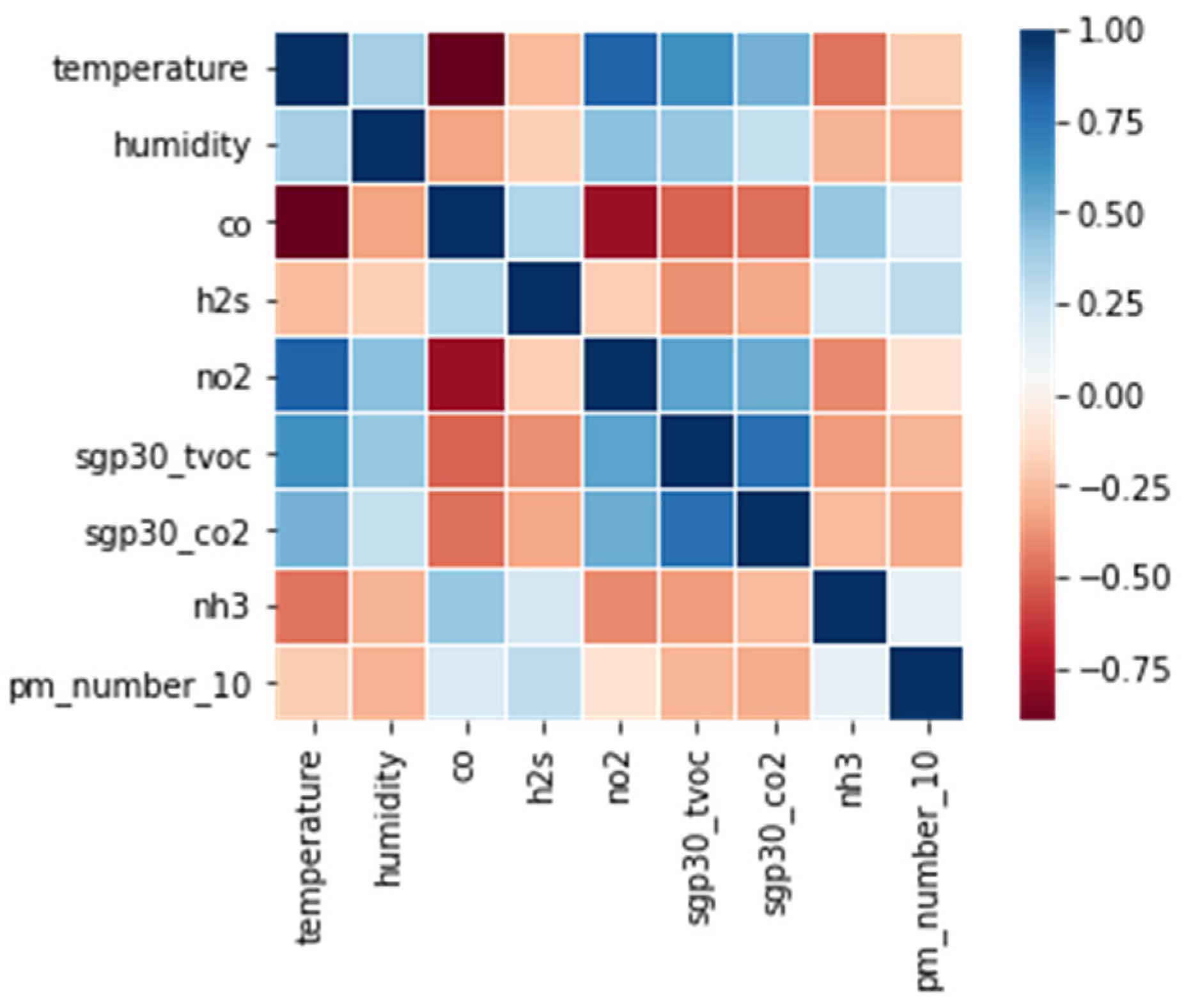
2.1. Experimental Setup and Dataset
2.2. Missing Data Imputation Methodology
2.3. Missing Data Type
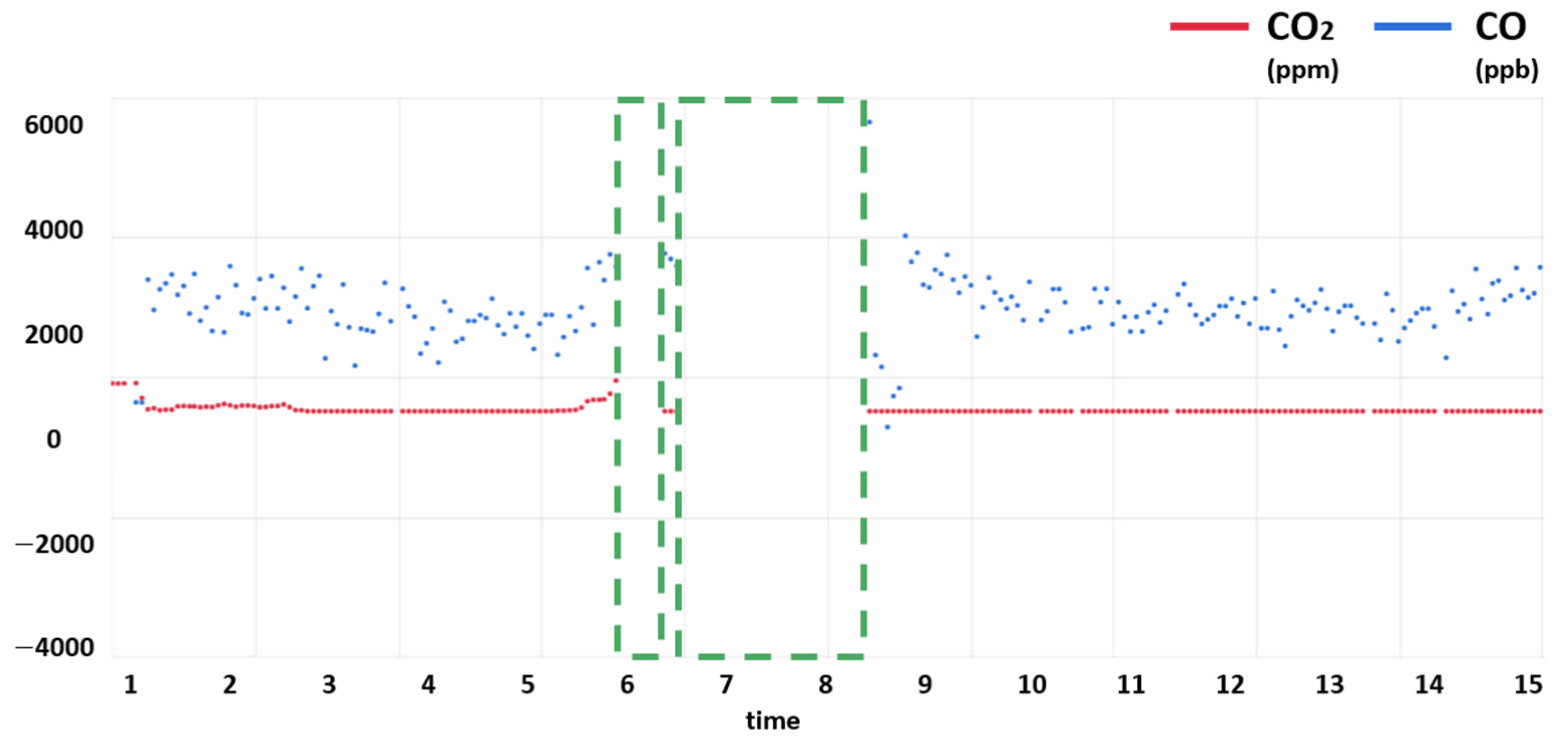
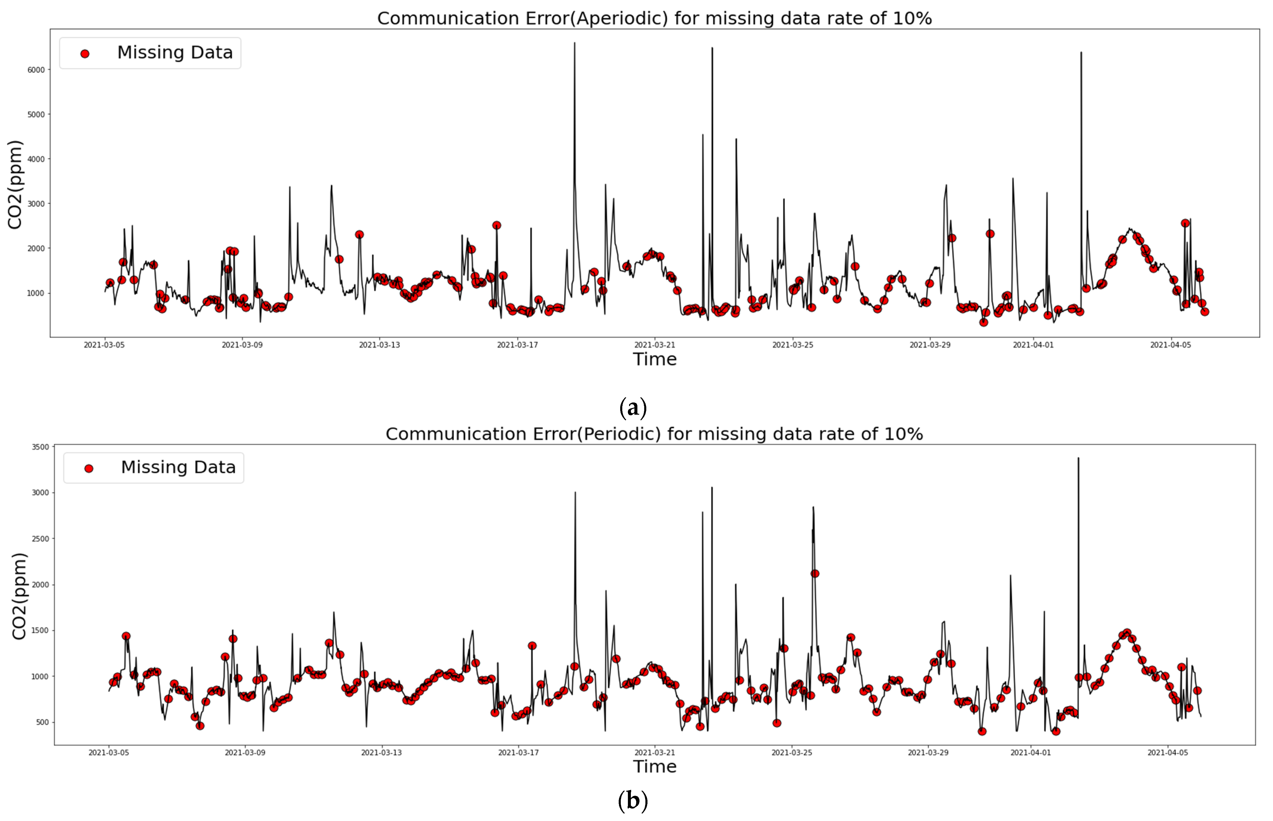
2.3.1. Communication Error Cases
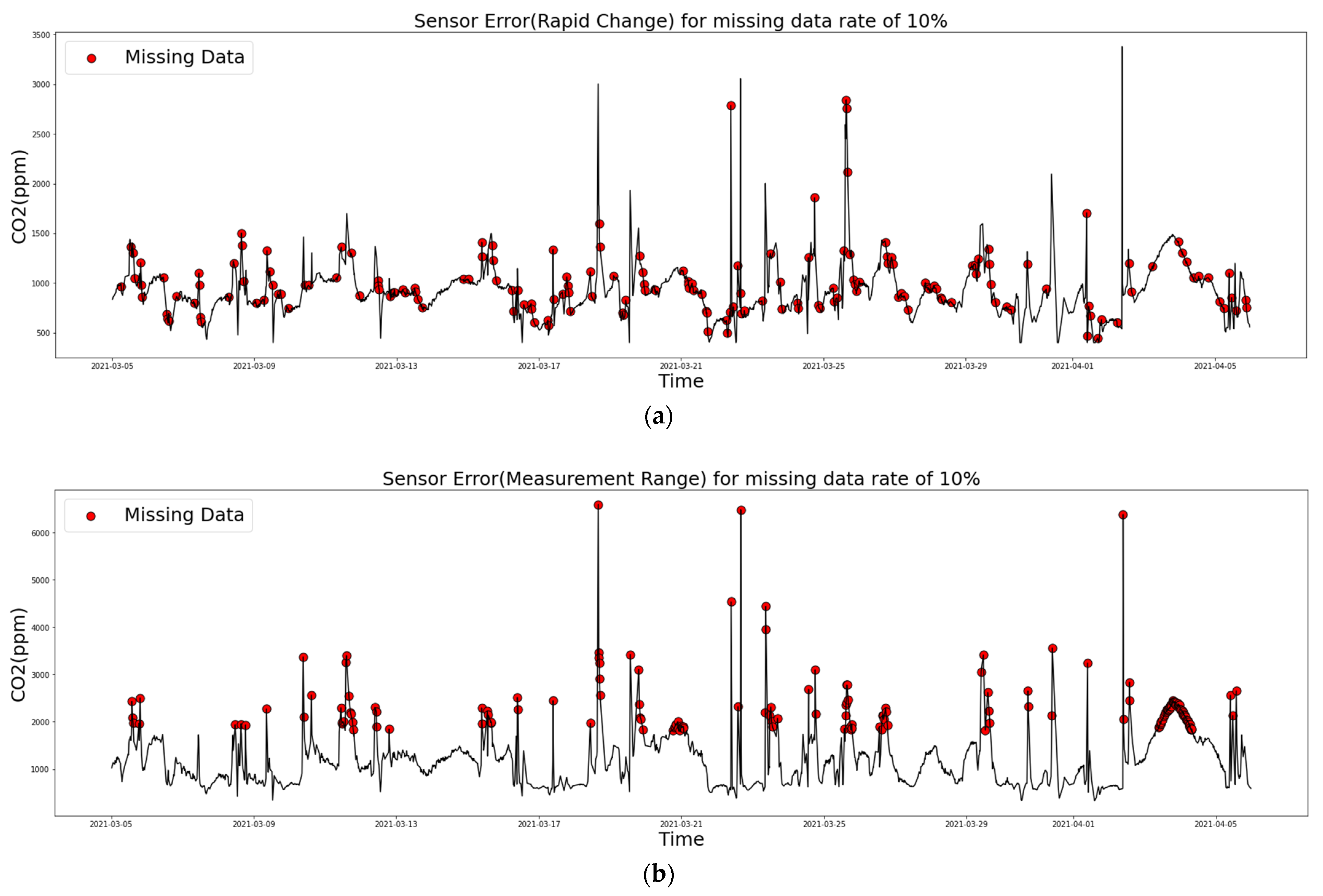
2.3.2. Sensor Error Cases
2.4. Missing Value Imputation by Single Model
2.4.1. Imputation in Univariate Data
- Last observation carried forward imputation (LOCF): Estimate missing values using data gathered just before the occurrence of missing values. This method is often used in longitudinal studies.
- Moving average imputation: Estimate the missing value as the average of a window of a certain size around the missing value. This technique is mainly used for time series data.
- Kalman imputation: Estimate missing values using Kalman smoothing. There was also a recent study on the treatment of missing values for local climate information [42].
2.4.2. Imputation in Multivariate Data
- K-NN imputation: The imputation of missing values using the k-values closest to the missing values. Based on this technique, a number of new, modified missing value imputation methods are emerging [43].
- Multiple linear regression: Fitting a multiple linear regression model and replacing missing values using this. This is used in the imputation method of missing values to measure pollution concentration and air quality [44].
- Random forest regression: Replacing missing values using the average predictions of multiple decision trees. Similar to K-NN, there are many new, modified missing value imputation methods based on random forest regression [45].
- Support vector regression: A method using a support vector machine, which is used to replace missing values.
- Miss forest: This is a random forest-based model, which is used to replace missing values. It can be used universally, regardless of continuous, categorical, or complex interactions and non-linear relationships [46].
2.5. Ensemble Learning Method
2.5.1. Weighted Average Method
2.5.2. Stacking Method
| Algorithm 1. Stacking Method. |
| 1: Step 1-1: univariate imputation 2: : univariate missing data, U: univariate imputer model 3: : imputed by U 4: Step 1-2: multivariate imputation 5: : multivariate data (no missing), : multivariate missing data, M: multivariate imputer model 6: train by T 7: : imputed by (M,) 8: Step 2: stacking method 9: : stack and , S: stacking imputer, : reference data 10: train by (R, Sd) 11: : imputed by S 12: : final prediction values |
2.6. Evaluation Method
3. Results
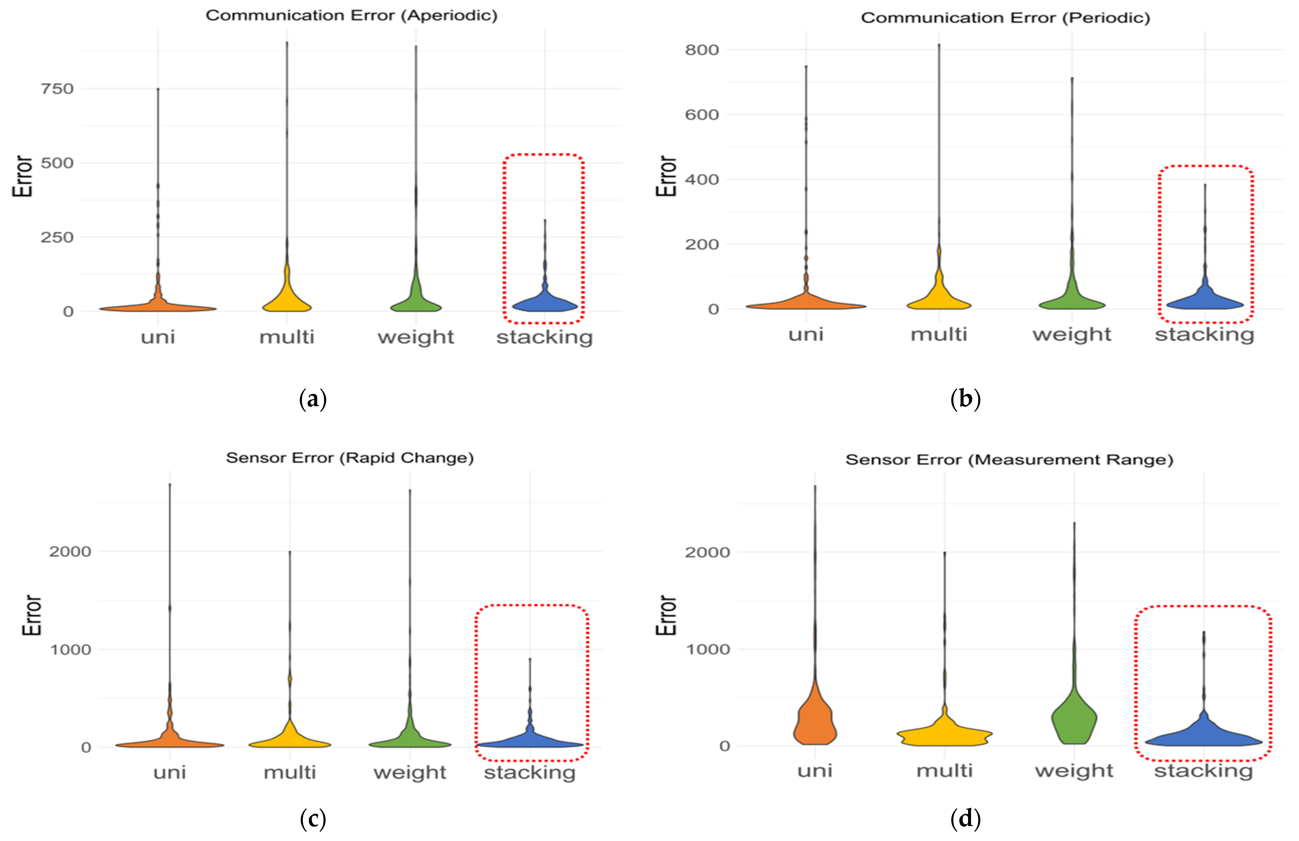
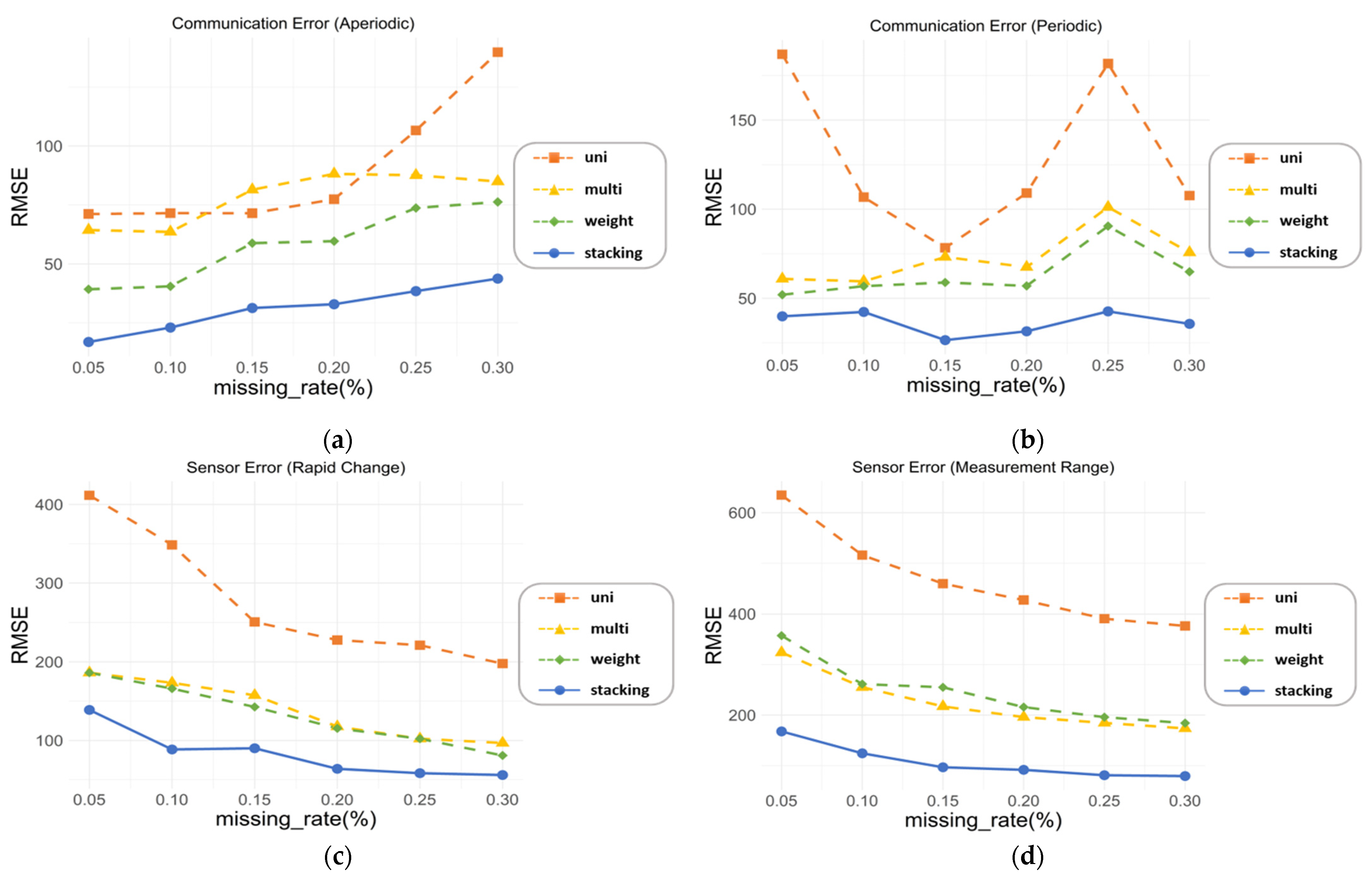
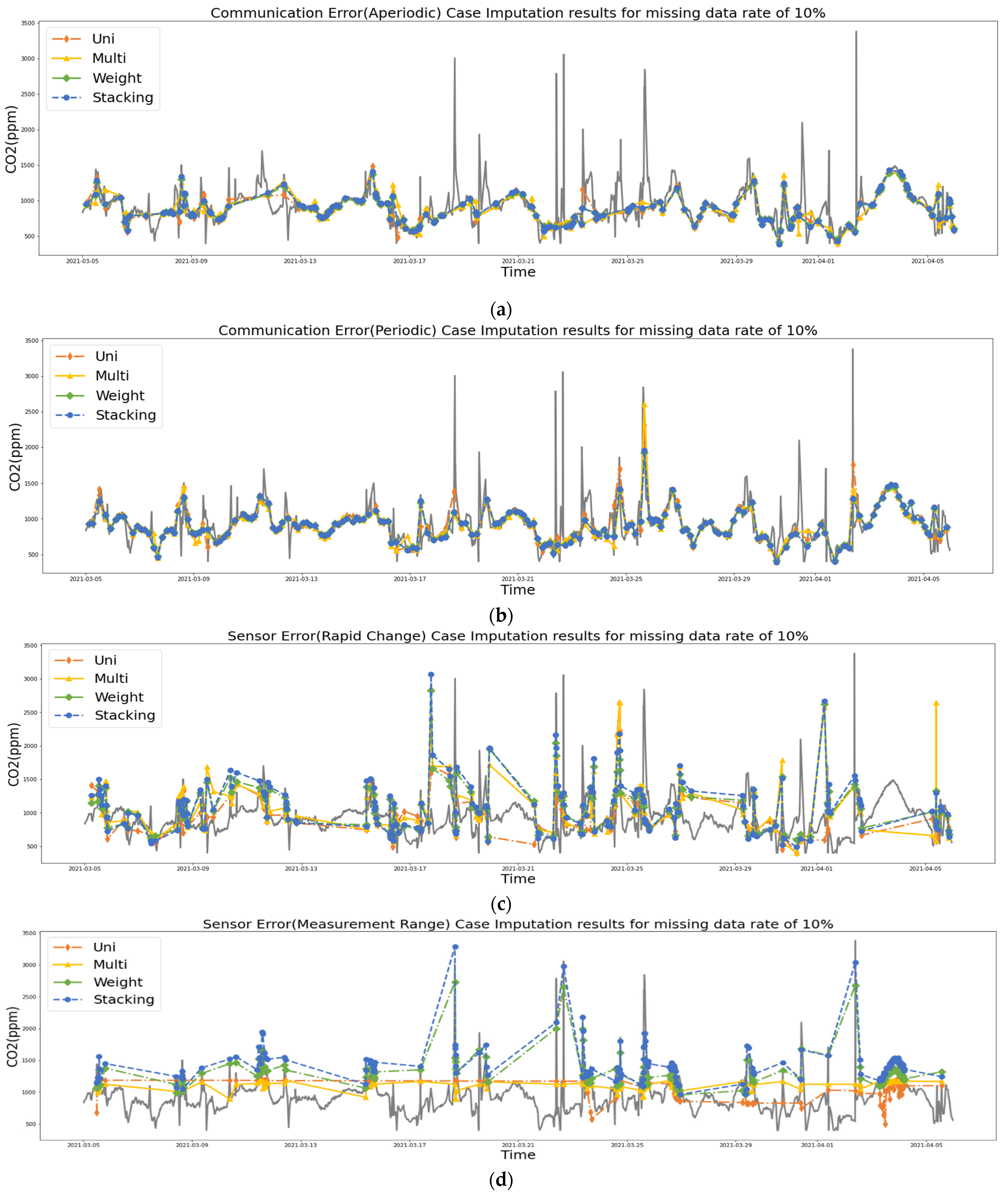
3.1. Differences between Models According to Evaluation Method
3.2. Performance Comparison between Models
4. Discussion
5. Conclusions
Author Contributions
Funding
Institutional Review Board Statement
Informed Consent Statement
Data Availability Statement
Acknowledgments
Conflicts of Interest
References
- Metia, S.; Ha, Q.; Duc, H.; Scorgie, Y. Urban air pollution estimation using unscented Kalman filtered inverse modeling with scaled monitoring data. Sustain. Cities Soc. 2020, 54, 101970. [Google Scholar] [CrossRef]
- Cho, J.; Joo, W. Data Clustering Method Using Efficient Fuzzifier Values Derivation. IEEE Access 2020, 8, 124624–124632. [Google Scholar] [CrossRef]
- Wang, J.; Dong, K. What drives environmental degradation? Evidence from 14 Sub-Saharan African countries. Sci. Total Environ. 2019, 656, 165–173. [Google Scholar] [CrossRef] [PubMed]
- WHO. Available online: https://www.who.int/vietnam/news/feature-stories/detail/ten-threats-to-global-health-in-2019 (accessed on 16 August 2021).
- Xu, X.; Nie, S.; Ding, H.; Hou, F.F. Environmental pollution and kidney diseases. Nat. Rev. Nephrol. 2018, 14, 313–324. [Google Scholar] [CrossRef] [PubMed]
- Liang, J.; Qin, Y.; Hong, Z. An Auto-exposure algorithm for detecting high contrast lighting conditions. In Proceedings of the 2007 7th International Conference on ASIC, Guilin, China, 22–25 October 2007; IEEE: Piscataway, NJ, USA, 2007; pp. 725–728. [Google Scholar]
- Liu, Y.; Dillon, T.; Yu, W.; Rahayu, W.; Mostafa, F. Missing Value Imputation for Industrial IoT Sensor Data with Large Gaps. IEEE Internet Things J. 2020, 7, 6855–6867. [Google Scholar] [CrossRef]
- Panapakidis, I.P.; Bouhouras, A.S.; Christoforidis, G.C. A missing data treatment method for photovoltaic installations. In Proceedings of the 2018 IEEE International Energy Conference (ENERGYCON), Limassol, Cyprus, 3–7 June 2018; IEEE: Piscataway, NJ, USA, 2018; pp. 1–6. [Google Scholar]
- Little, R.J.; Rubin, D.B. Statistical Analysis with Missing Data; John Wiley & Sons: Hoboken, NJ, USA, 2019. [Google Scholar]
- Cismondi, F.; Fialho, A.S.; Vieira, S.M.; Reti, S.R.; Sousa, J.M.C.; Finkelstein, S.N. Missing data in medical databases: Impute, delete or classify? Artif. Intell. Med. 2013, 58, 63–72. [Google Scholar] [CrossRef] [PubMed]
- Graham, J.W. Missing Data Analysis: Making It Work in the Real World. Annu. Rev. Psychol. 2009, 60, 549–576. [Google Scholar] [CrossRef] [PubMed] [Green Version]
- García-Laencina, P.J.; Sancho-Gómez, J.-L.; Figueiras, A.R. Pattern classification with missing data: A review. Neural Comput. Appl. 2009, 19, 263–282. [Google Scholar] [CrossRef]
- Sedghi, S.; Sadeghian, A.; Huang, B. Mixture semisupervised probabilistic principal component regression model with missing inputs. Comput. Chem. Eng. 2017, 103, 176–187. [Google Scholar] [CrossRef]
- Khatibisepehr, S.; Huang, B. Dealing with Irregular Data in Soft Sensors: Bayesian Method and Comparative Study. Ind. Eng. Chem. Res. 2008, 47, 8713–8723. [Google Scholar] [CrossRef]
- Magnani, M. Techniques for Dealing with Missing Data in Knowledge Discovery Tasks. 2004, Volume 15, p. 2007. Available online: http://magnanim.web.cs.unibo.it/index.html (accessed on 10 October 2021).
- Huamin, T.; Qiuqun, D.; Shanzhu, X. Reconstruction of time series with missing value using 2D representation-based denoising autoencoder. J. Syst. Eng. Electron. 2020, 31, 1087–1096. [Google Scholar] [CrossRef]
- Bhandari, S.; Bergmann, N.; Jurdak, R.; Kusy, B. Time Series Analysis for Spatial Node Selection in Environment Monitoring Sensor Networks. Sensors 2017, 18, 11. [Google Scholar] [CrossRef] [PubMed] [Green Version]
- Moritz, S.; Sardá, A.; Bartz-Beielstein, T.; Zaefferer, M.; Stork, J. Comparison of different methods for univariate time series imputation in R. arXiv 2015, arXiv:1510.03924. [Google Scholar]
- Baddoo, T.; Li, Z.; Odai, S.; Boni, K.; Nooni, I.; Andam-Akorful, S. Comparison of Missing Data Infilling Mechanisms for Recovering a Real-World Single Station Streamflow Observation. Int. J. Environ. Res. Public Health 2021, 18, 8375. [Google Scholar] [CrossRef] [PubMed]
- Yan, X.; Xiong, W.; Hu, L.; Wang, F.; Zhao, K. Missing Value Imputation Based on Gaussian Mixture Model for the Internet of Things. Math. Probl. Eng. 2015, 2015, 1–8. [Google Scholar] [CrossRef]
- Park, J.; Kim, S. Improved Interpolation and Anomaly Detection for Personal PM2.5 Measurement. Appl. Sci. 2020, 10, 543. [Google Scholar] [CrossRef] [Green Version]
- Chen, L.-J.; Ho, Y.-H.; Hsieh, H.-H.; Huang, S.-T.; Lee, H.-C.; Mahajan, S. ADF: An Anomaly Detection Framework for Large-Scale PM2.5 Sensing Systems. IEEE Internet Things J. 2018, 5, 559–570. [Google Scholar] [CrossRef]
- Apostol, E.-S.; Truică, C.-O.; Pop, F.; Esposito, C. Change Point Enhanced Anomaly Detection for IoT Time Series Data. Water 2021, 13, 1633. [Google Scholar] [CrossRef]
- Crespo Turrado, C.; Sánchez Lasheras, F.; Calvo-Rollé, J.L.; Piñón-Pazos, A.J.; de Cos Juez, F.J. A New Missing Data Imputation Algorithm Applied to Electrical Data Loggers. Sensors 2015, 15, 31069–31082. [Google Scholar] [CrossRef] [Green Version]
- Kim, T.; Ko, W.; Kim, J.; Kim, T. Analysis and Impact Evaluation of Missing Data Imputation in Day-ahead PV Generation Forecasting. Appl. Sci. 2019, 9, 204. [Google Scholar] [CrossRef] [Green Version]
- Batista, G.; Monard, M.C. An analysis of four missing data treatment methods for supervised learning. Appl. Artif. Intell. 2003, 17, 519–533. [Google Scholar] [CrossRef]
- Banks, D.; House, L.; McMorris, F.R.; Arabie, P.; Gaul, W.A. Classification, Clustering, and Data Mining Applications. In Proceedings of the Meeting of the International Federation of Classification Societies (IFCS), Illinois Institute of Technology, Chicago, IL, USA, 15–18 July 2004; Springer Science & Business Media: Germany, Berlin, 2011. [Google Scholar]
- Luengo, J.; García, S.; Herrera, F. A study on the use of imputation methods for experimentation with radial basis function network classifiers handling missing attribute values: The good synergy between rbfns and eventcovering method. Neural Netw. 2010, 23, 406–418. [Google Scholar] [CrossRef] [PubMed]
- Brock, G.N.; Shaffer, J.R.; E Blakesley, R.; Lotz, M.J.; Tseng, G.C. Which missing value imputation method to use in expression profiles: A comparative study and two selection schemes. BMC Bioinform. 2008, 9, 12. [Google Scholar] [CrossRef] [PubMed] [Green Version]
- Xia, J.; Zhang, S.; Cai, G.; Li, L.; Pan, Q.; Yan, J.; Ning, G. Adjusted weight voting algorithm for random forests in handling missing values. Pattern Recognit. 2017, 69, 52–60. [Google Scholar] [CrossRef]
- Burgette, L.F.; Reiter, J.P. Multiple Imputation for Missing Data via Sequential Regression Trees. Am. J. Epidemiol. 2010, 172, 1070–1076. [Google Scholar] [CrossRef] [PubMed]
- Kang, P. Locally linear reconstruction based missing value imputation for supervised learning. Neurocomputing 2013, 118, 65–78. [Google Scholar] [CrossRef]
- Gautam, C.; Ravi, V. Data imputation via evolutionary computation, clustering and a neural network. Neurocomputing 2015, 156, 134–142. [Google Scholar] [CrossRef]
- Silva-Ramírez, E.-L.; Pino-Mejías, R.; López-Coello, M. Single imputation with multilayer perceptron and multiple imputation combining multilayer perceptron and k-nearest neighbours for monotone patterns. Appl. Soft Comput. 2015, 29, 65–74. [Google Scholar] [CrossRef]
- Ahsan, M.; Based, M.; Haider, J.; Rodrigues, E.M. Smart Monitoring and Controlling of Appliances Using LoRa Based IoT System. Designs 2021, 5, 17. [Google Scholar] [CrossRef]
- Basford, P.J.; Bulot, F.M.J.; Apetroaie-Cristea, M.; Cox, S.J.; Ossont, S.J.J. LoRaWAN for Smart City IoT Deployments: A Long Term Evaluation. Sensors 2020, 20, 648. [Google Scholar] [CrossRef] [Green Version]
- Cho, J. Efficient Autonomous Defense System Using Machine Learning on Edge Device. CMC-Computers 2022, 70, 3565–3588. [Google Scholar] [CrossRef]
- Browning, B.L.; Browning, S. Genotype Imputation with Millions of Reference Samples. Am. J. Hum. Genet. 2016, 98, 116–126. [Google Scholar] [CrossRef] [PubMed] [Green Version]
- Li, Y.; Li, J.; Zhang, M.; Li, Y.; Zou, P. Improving Neural Machine Translation with Linear Interpolation of a Short-Path Unit. ACM Trans. Asian Low-Resour. Lang. Inf. Process. 2020, 19, 1–16. [Google Scholar] [CrossRef] [Green Version]
- Karim, S.A.A.; Ismail, M.T.; Othman, M.; Abdullah, M.F.; Hasan, M.K.; Sulaiman, J. Rational cubic spline interpolation for missing solar data imputation. J. Eng. Appl. Sci. 2018, 13, 2587–2592. [Google Scholar]
- Keller, W.; Borkowski, A. Thin plate spline interpolation. J. Geod. 2019, 93, 1251–1269. [Google Scholar] [CrossRef]
- Saputra, M.D.; Hadi, A.F.; Riski, A.; Anggraeni, D. Handling Missing Values and Unusual Observations in Statistical Downscaling Using Kalman Filter. J. Phys. Conf. Ser. 2021, 1863, 012035. [Google Scholar] [CrossRef]
- Huang, J.; Keung, J.; Sarro, F.; Li, Y.-F.; Yu, Y.; Chan, W.K.; Sun, H. Cross-validation based K nearest neighbor imputation for software quality datasets: An empirical study. J. Syst. Softw. 2017, 132, 226–252. [Google Scholar] [CrossRef] [Green Version]
- Shahbazi, H.; Karimi, S.; Hosseini, V.; Yazgi, D.; Torbatian, S. A novel regression imputation framework for Tehran air pollution monitoring network using outputs from WRF and CAMx models. Atmos. Environ. 2018, 187, 24–33. [Google Scholar] [CrossRef]
- Kokla, M.; Virtanen, J.; Kolehmainen, M.; Paananen, J.; Hanhineva, K. Random forest-based imputation outperforms other methods for imputing LC-MS metabolomics data: A comparative study. BMC Bioinform. 2019, 20, 1–11. [Google Scholar] [CrossRef] [PubMed] [Green Version]
- Stekhoven, D.J.; Bühlmann, P. MissForest—non-parametric missing value imputation for mixed-type data. Bioinformatics 2012, 28, 112–118. [Google Scholar] [CrossRef] [PubMed] [Green Version]
- Li, J.; Yu, Y.; Qing, X. Embedded FBG Sensor Based Impact Identification of CFRP Using Ensemble Learning. Sensors 2021, 21, 1452. [Google Scholar] [CrossRef] [PubMed]
- Xu, Y.; Meng, R.; Zhao, X. Research on a Gas Concentration Prediction Algorithm Based on Stacking. Sensors 2021, 21, 1597. [Google Scholar] [CrossRef] [PubMed]
- Li, L.; Li, Y.; Li, Z. Efficient missing data imputing for traffic flow by considering temporal and spatial dependence. Transp. Res. Part C Emerg. Technol. 2013, 34, 108–120. [Google Scholar] [CrossRef]
- Smith, B.L.; Scherer, W.T.; Conklin, J.H. Exploring Imputation Techniques for Missing Data in Transportation Management Systems. Transp. Res. Rec. J. Transp. Res. Board 2003, 1836, 132–142. [Google Scholar] [CrossRef]
- Chen, M.; Xia, J.; Liu, R.R. Developing a Strategy for Imputing Missing Traffic Volume Data. J. Transp. Res. Forum 2010, 45. [Google Scholar] [CrossRef]
- Chai, T.; Draxler, R.R. Root mean square error (RMSE) or mean absolute error (MAE)?—Arguments against avoiding RMSE in the literature. Geosci. Model Dev. 2014, 7, 1247–1250. [Google Scholar] [CrossRef] [Green Version]


| Sensor Model | Sensor Type | Sensing Target | Detection Range |
|---|---|---|---|
| SPS 30 | Optical | PM1, PM2.5, PM4, PM10 | 1–1000 μg/m3 |
| SVM 30 | Semiconductor | TVOC, CO2, Temperature, Humidity | TVOC: 0~60 ppm, CO2: 0~60,000 ppm, Temperature: –20~85 °C, Humidity: 0~100% RH |
| DGS-CO 968-034 | Electrochemical | CO | 0–1000 ppm |
| DGS-H2S 968-036 | H2S | 0–10 ppm | |
| DGS-NO2 968-043 | NO2 | 0–5 ppm | |
| FECS44-100 | NH3 | 0–100 ppm |
| Case | Missing Type | Missingness Mechanism |
|---|---|---|
| Communication error | Aperiodic | MCAR |
| Periodic | MCAR | |
| Sensor error | Rapid change | NMAR |
| Measurement Range | NMAR |
| Evaluation Method | Equation | Perfect Score | Data Distribution |
|---|---|---|---|
| Mean Absolute Error (MAE) | MAE = | 0 | Uniform distribution |
| Root Mean Square Error (RMSE) | RMSE = | 0 | Normal distribution |
| Case | Existing Model | Proposed Model | ||
|---|---|---|---|---|
| Univariate | Multivariate | Weighted Average | Stacking | |
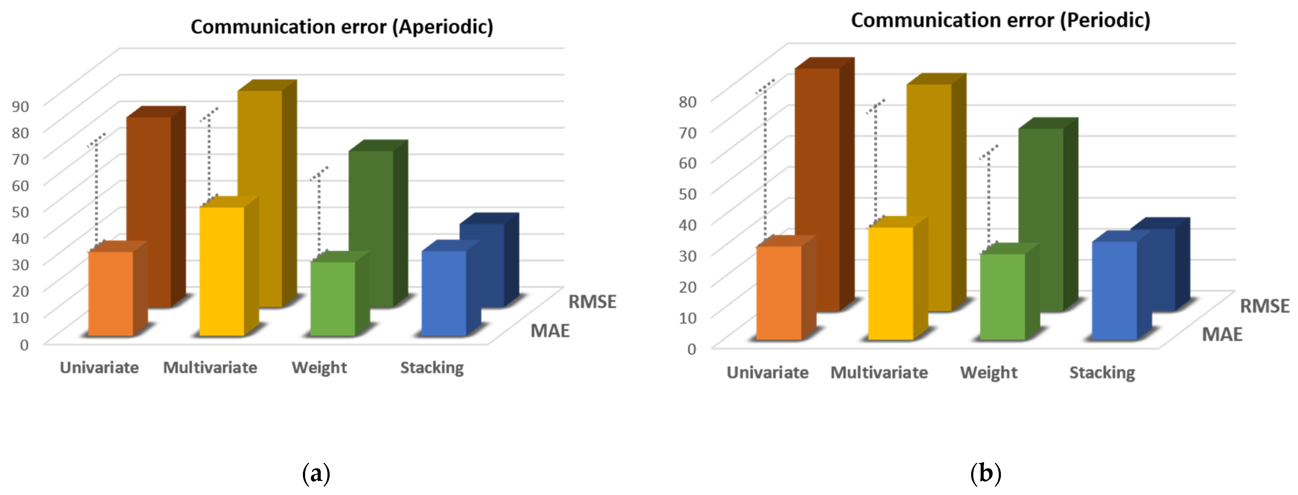
| Communication error (aperiodic) | 71.51 | 63.57 | 40.48 | 23.00 |
| Communication error (periodic) | 106.73 | 59.52 | 56.82 | 42.33 |
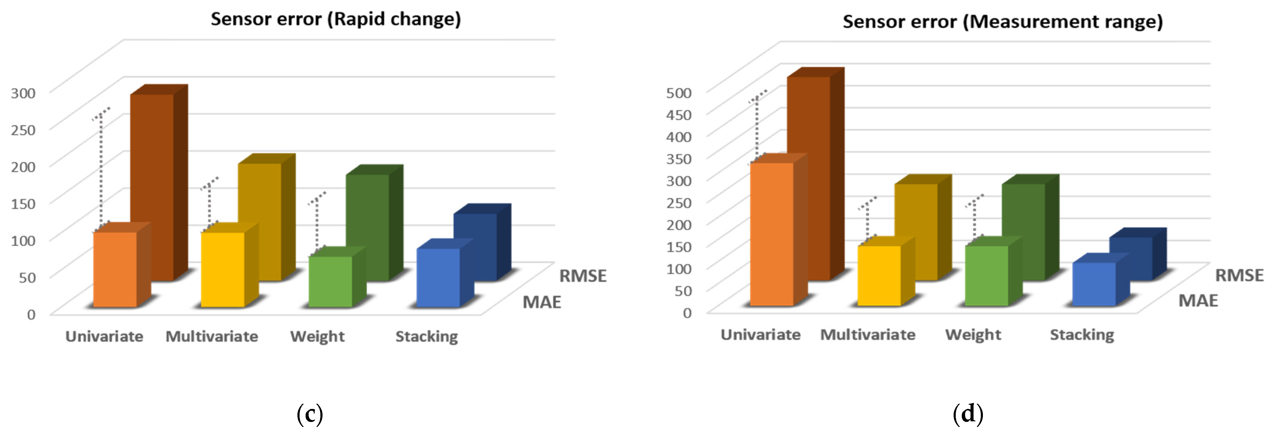
| Sensor error (rapid change) | 348.51 | 173.37 | 165.97 | 88.53 |
| Sensor error (measurement range) | 515.92 | 255.14 | 298.88 | 124.31 |
| Case | Existing Model | Proposed Model | ||
|---|---|---|---|---|
| Univariate (A) | Multivariate (B) | Weighted Average (C) (C-A-B) | Stacking (D) (D-A-B) | |
| Communication error (aperiodic) | 0.009 | 0.814 | 0.847 | 0.836 |
| (0.024) | (0.013) | |||
| Communication error (periodic) | 0.009 | 0.814 | 0.837 | 0.842 |
| (0.014) | (0.019) | |||
| Sensor error (rapid change) | 0.009 | 0.808 | 0.840 | 0.831 |
| (0.023) | (0.014) | |||
| Sensor error (measurement range) | 0.008 | 0.807 | 0.826 | 0.836 |
| (0.011) | (0.021) | |||
Publisher’s Note: MDPI stays neutral with regard to jurisdictional claims in published maps and institutional affiliations. |
© 2021 by the authors. Licensee MDPI, Basel, Switzerland. This article is an open access article distributed under the terms and conditions of the Creative Commons Attribution (CC BY) license (https://creativecommons.org/licenses/by/4.0/).
Share and Cite
Choi, C.; Jung, H.; Cho, J. An Ensemble Method for Missing Data of Environmental Sensor Considering Univariate and Multivariate Characteristics. Sensors 2021, 21, 7595. https://doi.org/10.3390/s21227595
Choi C, Jung H, Cho J. An Ensemble Method for Missing Data of Environmental Sensor Considering Univariate and Multivariate Characteristics. Sensors. 2021; 21(22):7595. https://doi.org/10.3390/s21227595
Chicago/Turabian StyleChoi, Chanyoung, Haewoong Jung, and Jaehyuk Cho. 2021. "An Ensemble Method for Missing Data of Environmental Sensor Considering Univariate and Multivariate Characteristics" Sensors 21, no. 22: 7595. https://doi.org/10.3390/s21227595
APA StyleChoi, C., Jung, H., & Cho, J. (2021). An Ensemble Method for Missing Data of Environmental Sensor Considering Univariate and Multivariate Characteristics. Sensors, 21(22), 7595. https://doi.org/10.3390/s21227595