
FGSC: Fuzzy Guided Scale Choice SSD Model for Edge AI Design on Real-Time Vehicle Detection and Class Counting


 , , and
Abstract
:1. Introduction
- ❖
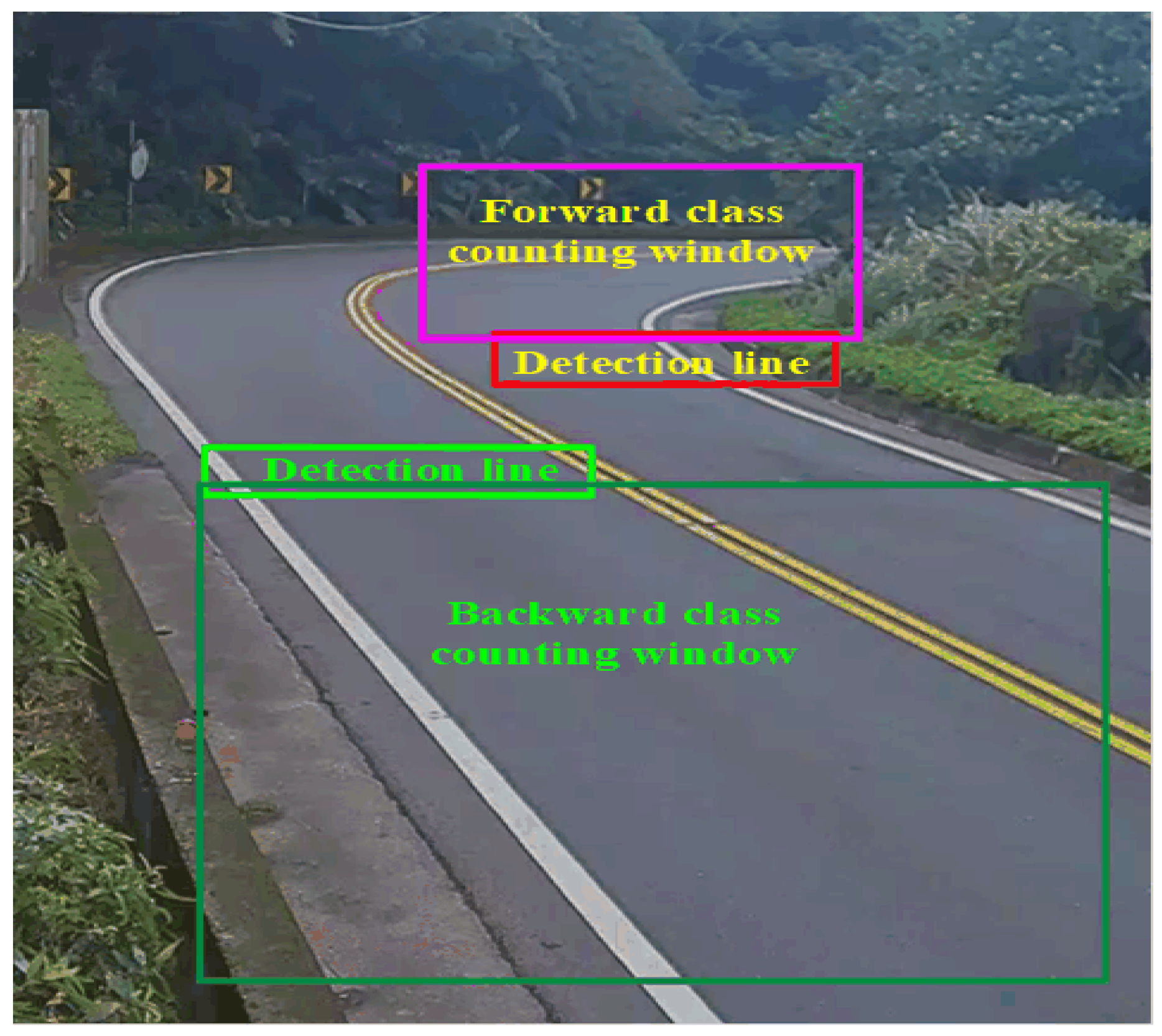
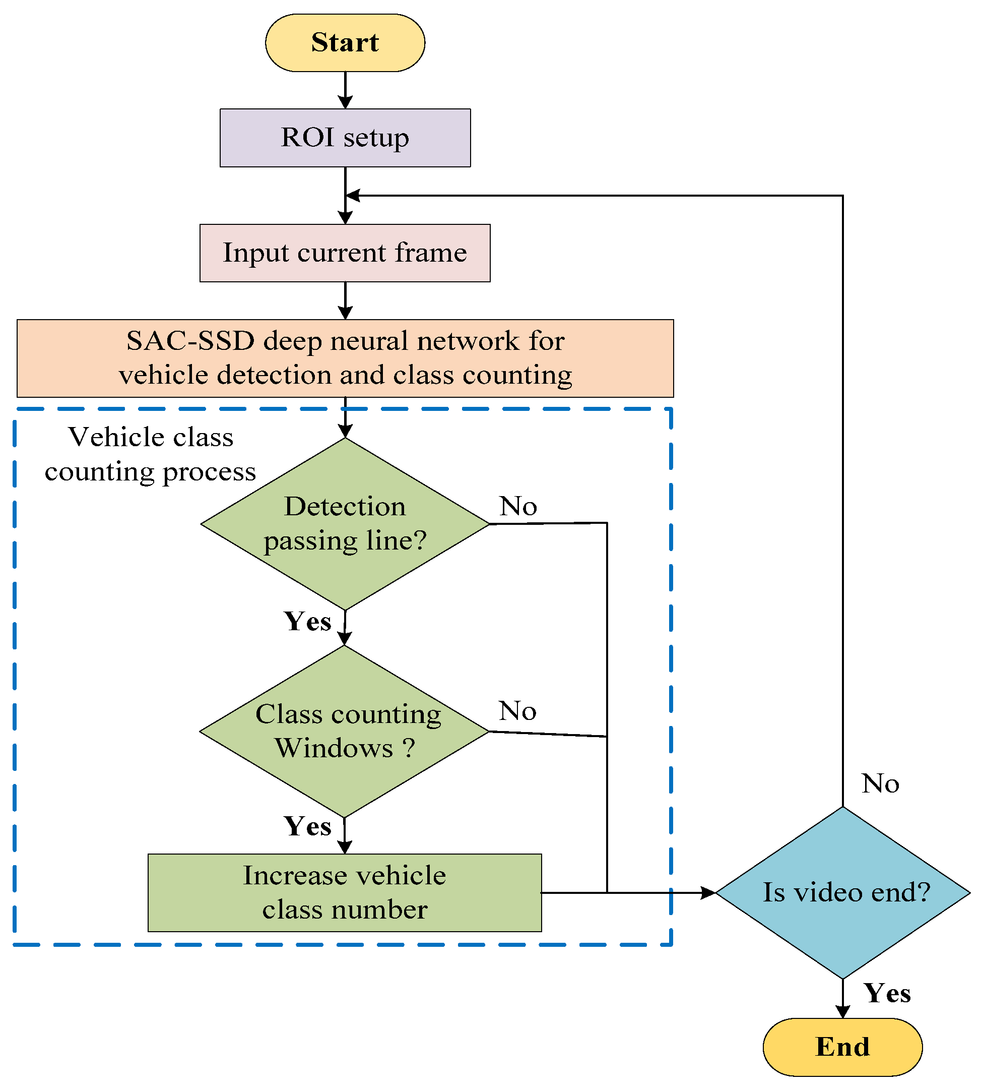
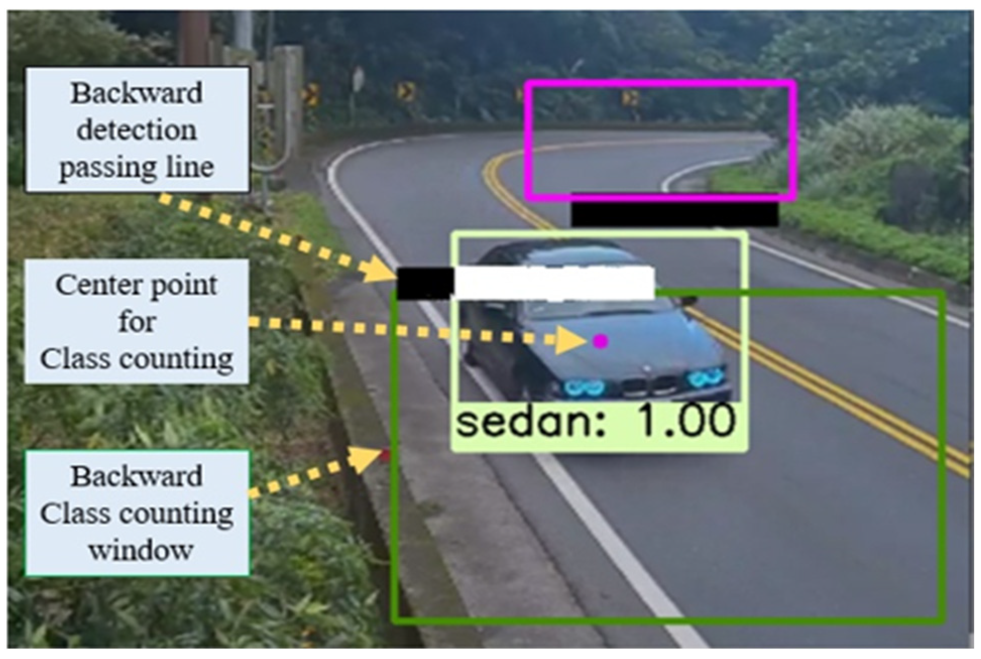
- We set up the Region of Interest (ROI) for quick vehicle detection and class counting from forward passing and backward passing lanes.
- ❖
- Proposed FGSC blocks distinguish between significant and irrelevant features. Next, improved system operation speed by skipping unnecessary characteristics.
- ❖
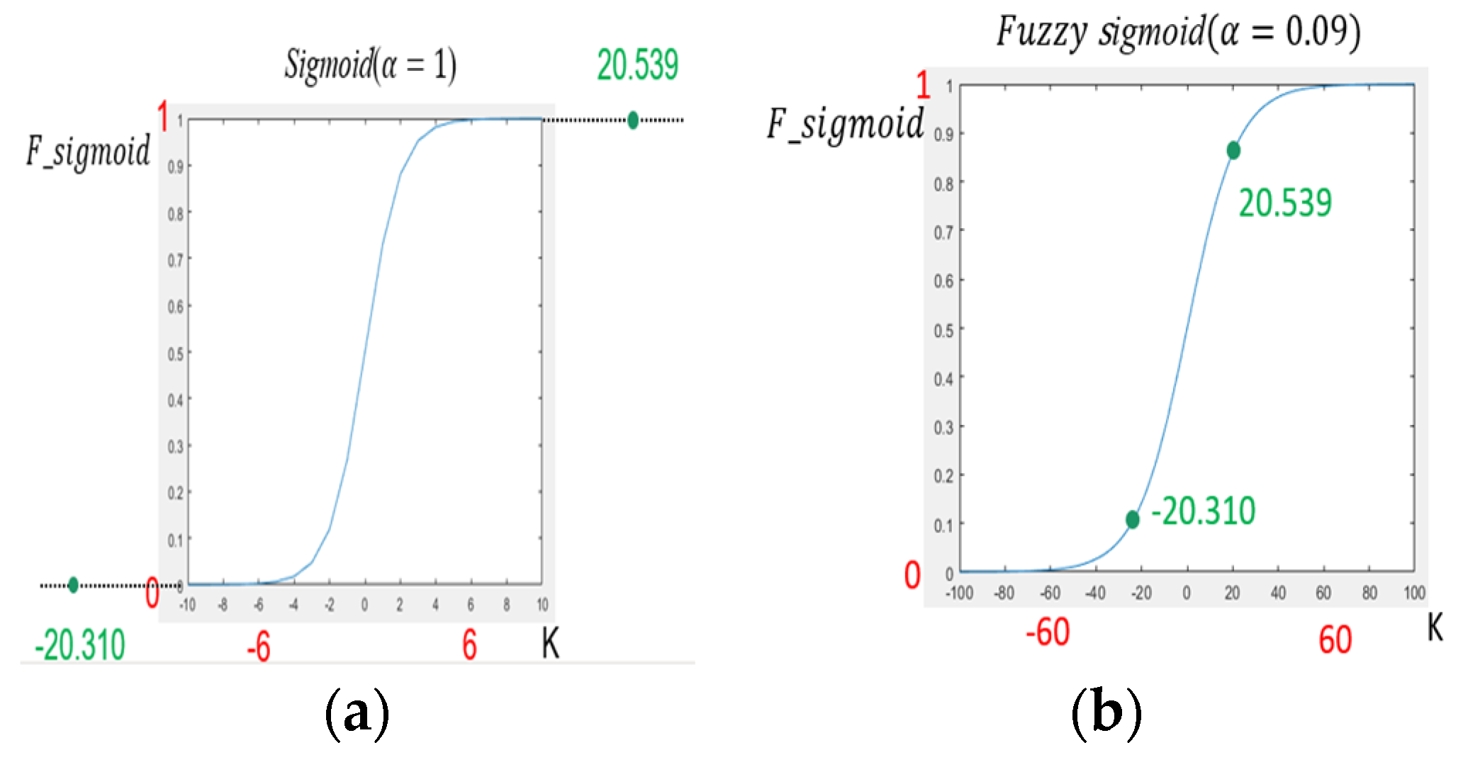
- We have developed a fuzzy sigmoid function for controlling the activation interval and avoiding saturated output feature values.
- ❖
- In comparison to the SSD model, the proposed FGSC-SSD model has achieved higher speed under the same detection accuracy for the PASCAL VOC dataset and Benchmark BIT Vehicle dataset.
2. Related Works
3. Proposed Vehicle Detection and Class Counting System
3.1. ROI Setup
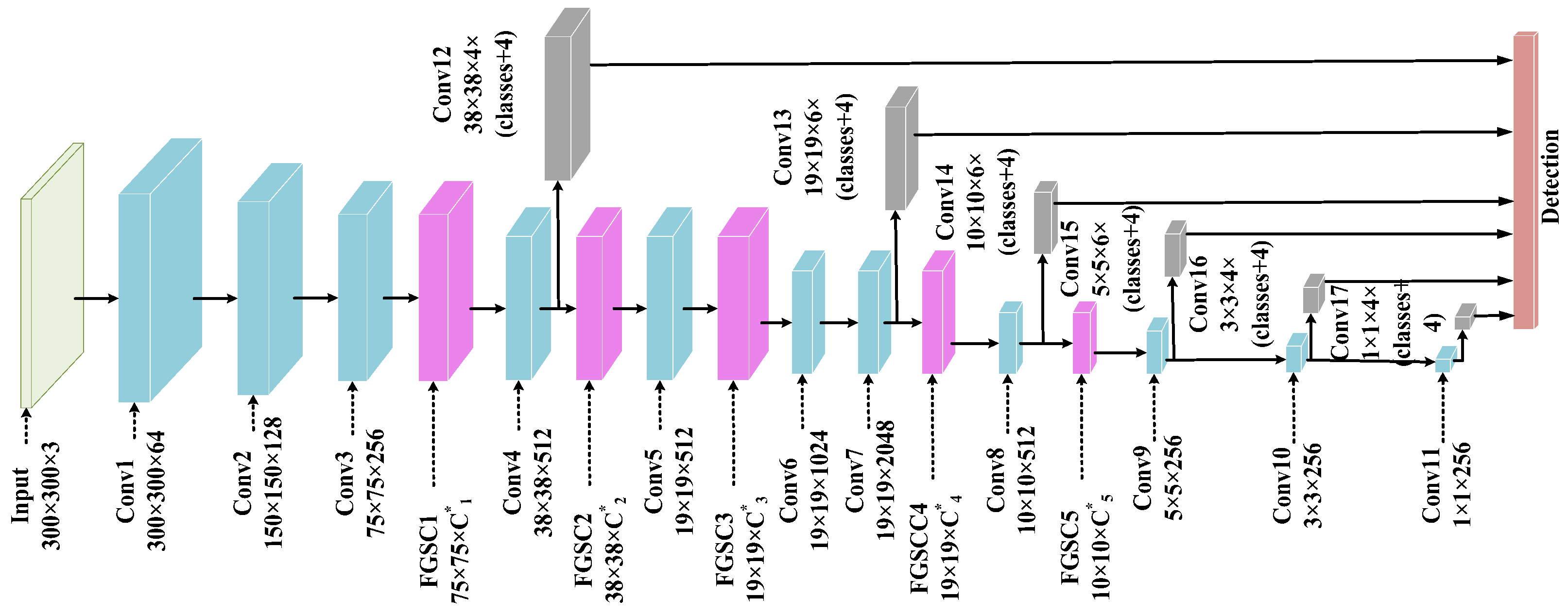
3.2. FGSC-SSD Model Architecture
3.3. FGSC Block Operation Function
3.3.1. Global Intensity Function
3.3.2. Fuzzy Guided
- Fully Connected
- Fuzzy Sigmoid Function
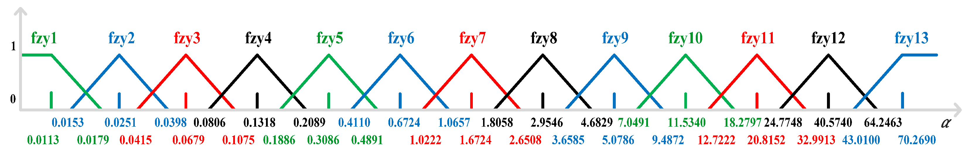
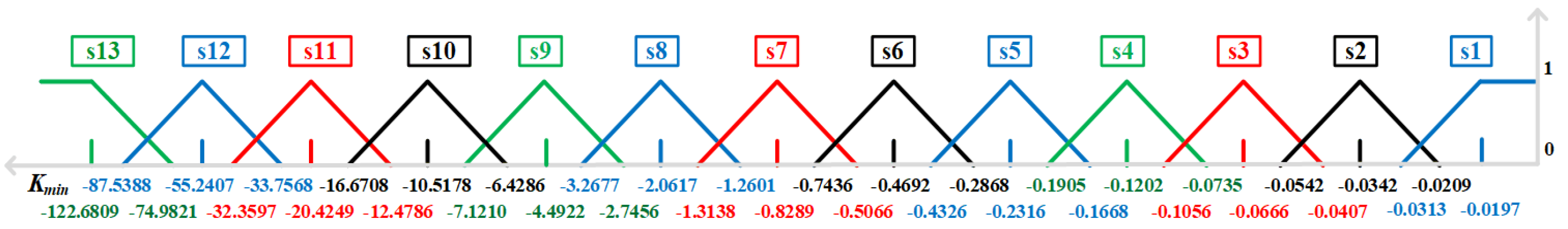
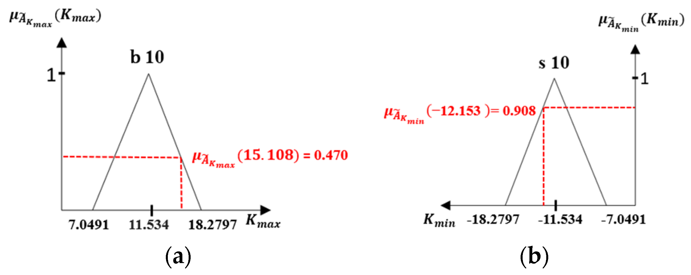
- The Fuzzy Sets for
- 2.
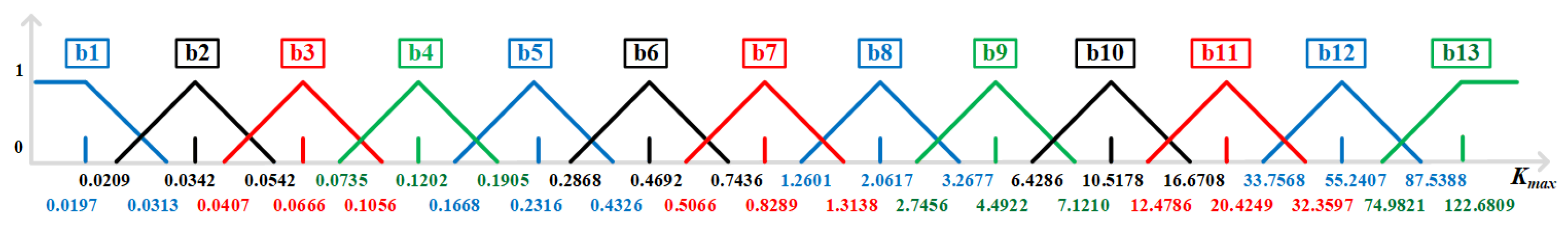
- The Fuzzy Sets for and
- 3.
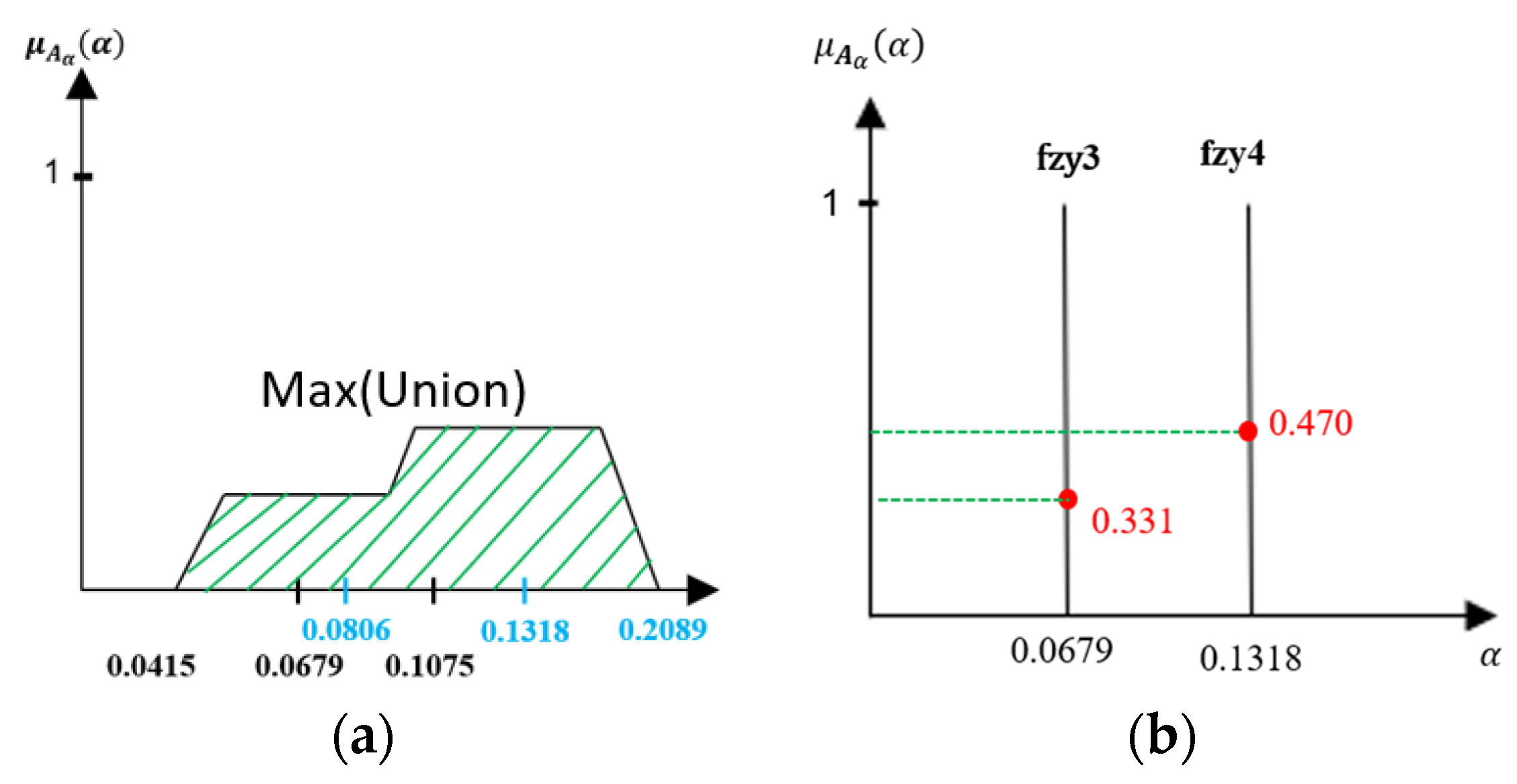
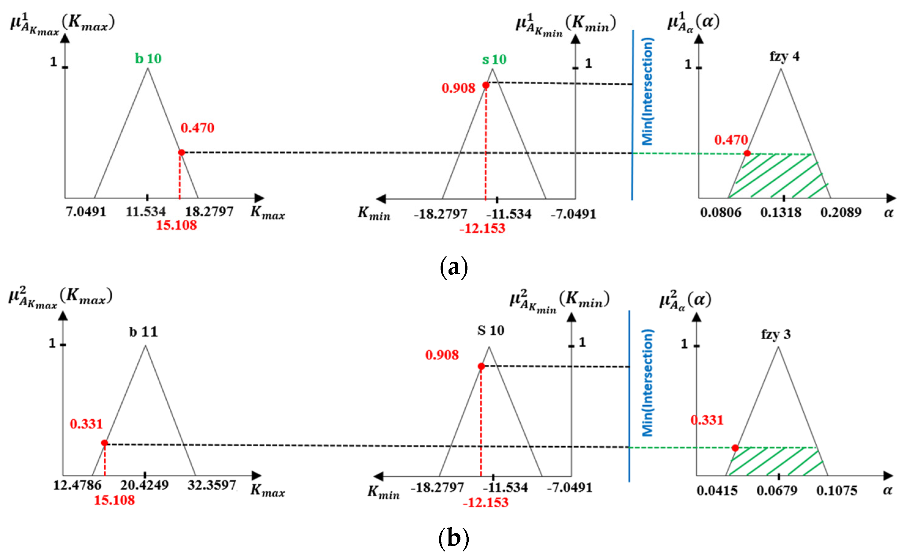
- The Fuzzy Logic Processing
- 4.
- Fuzzification
- 5.
- Rulesets
- 6.
- Inference Process
- 7.
- Defuzzification
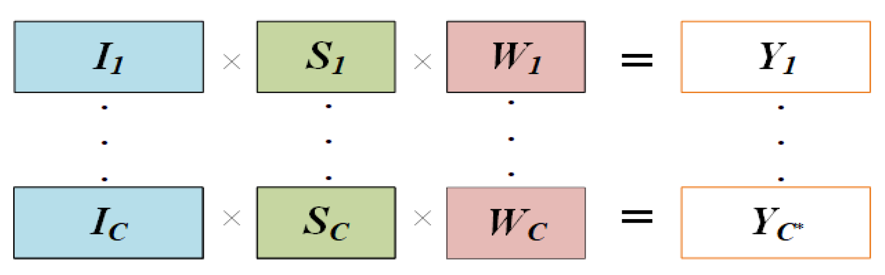
3.3.3. Scale Choice
- Operation Choice Mechanism
| Algorithm 1Operation choice mechanism. |
| , output , Output: 1 Set = 0.2 2 Set 3 for c = 1: do 4 if > do 5 6 ++ 7 end end |
- Effects of Different Jump-threshold
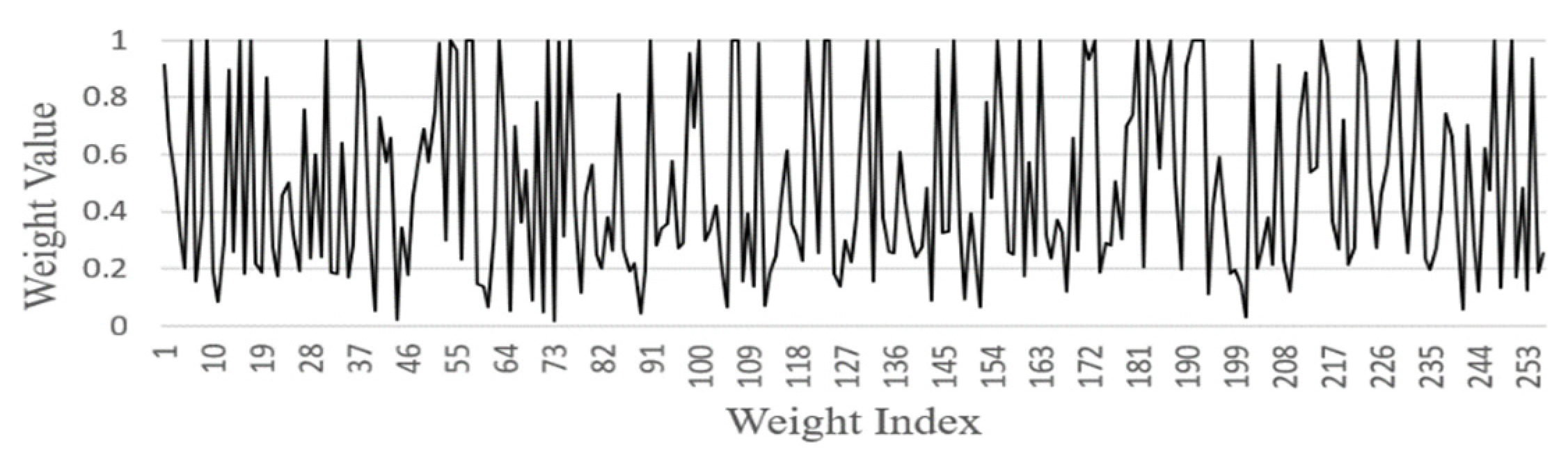
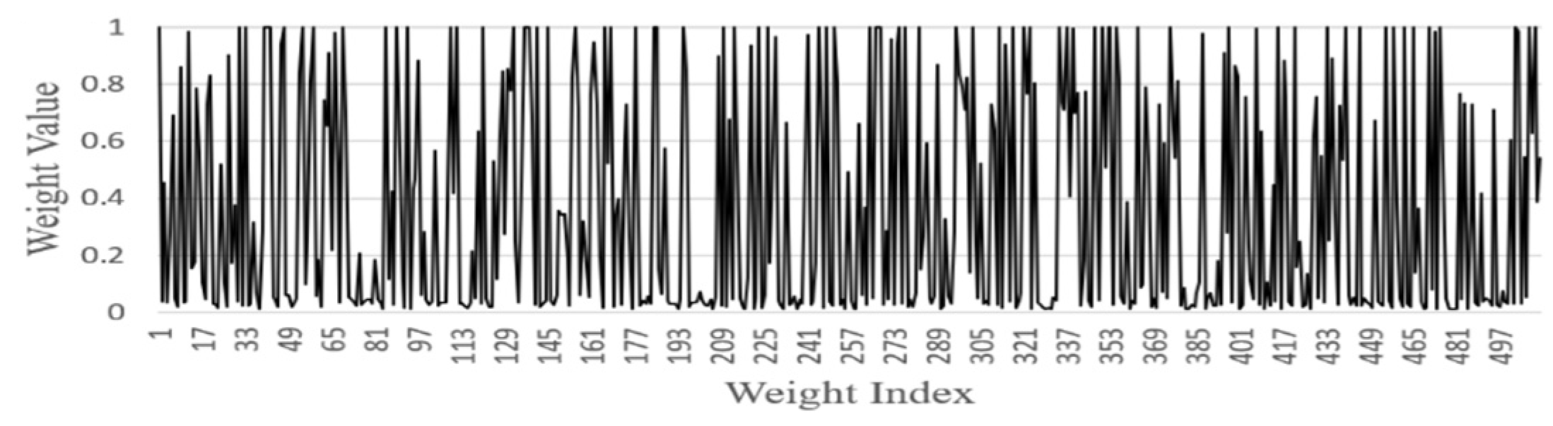
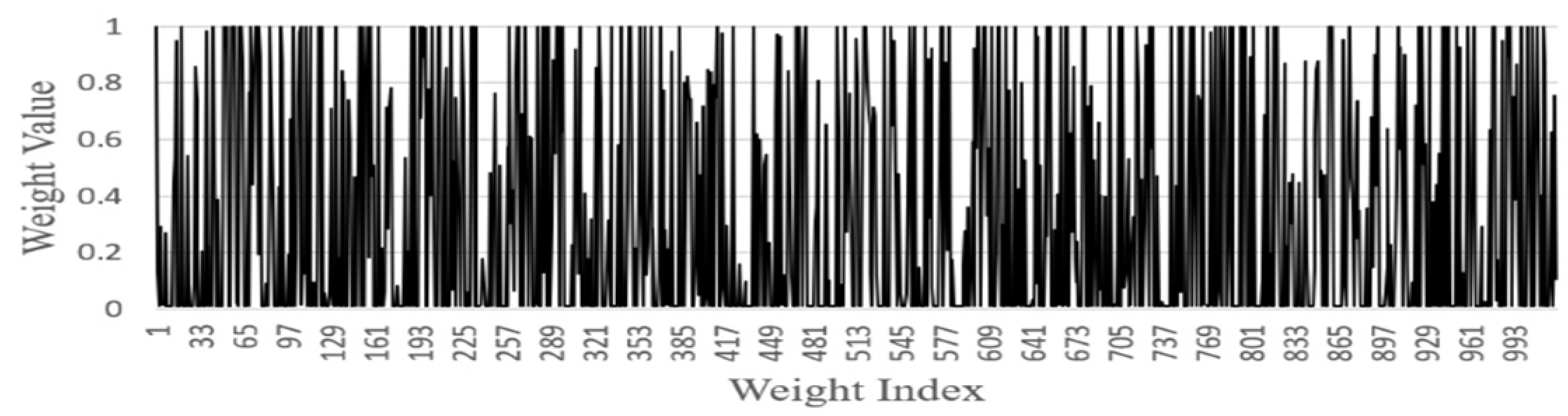
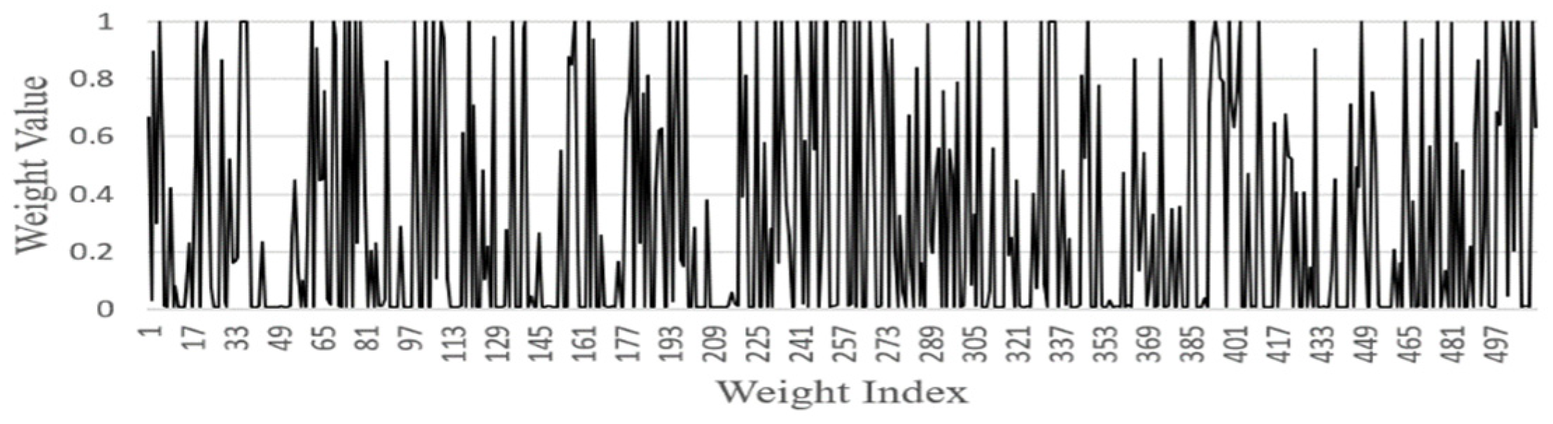
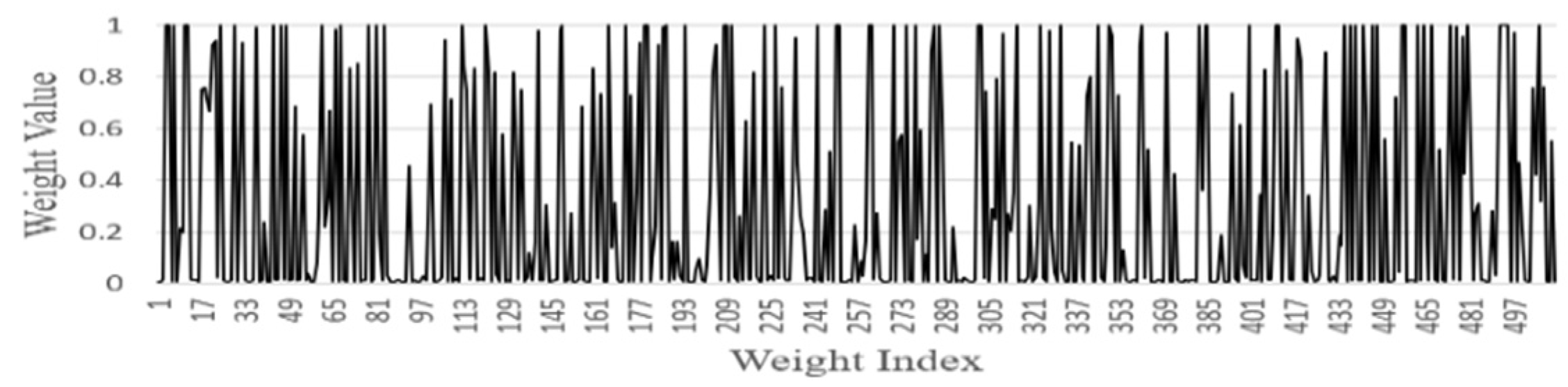
- FGSC Block Weights distribution
4. Vehicle Detection and Class Counting Process
4.1. Vehicle Detection Process
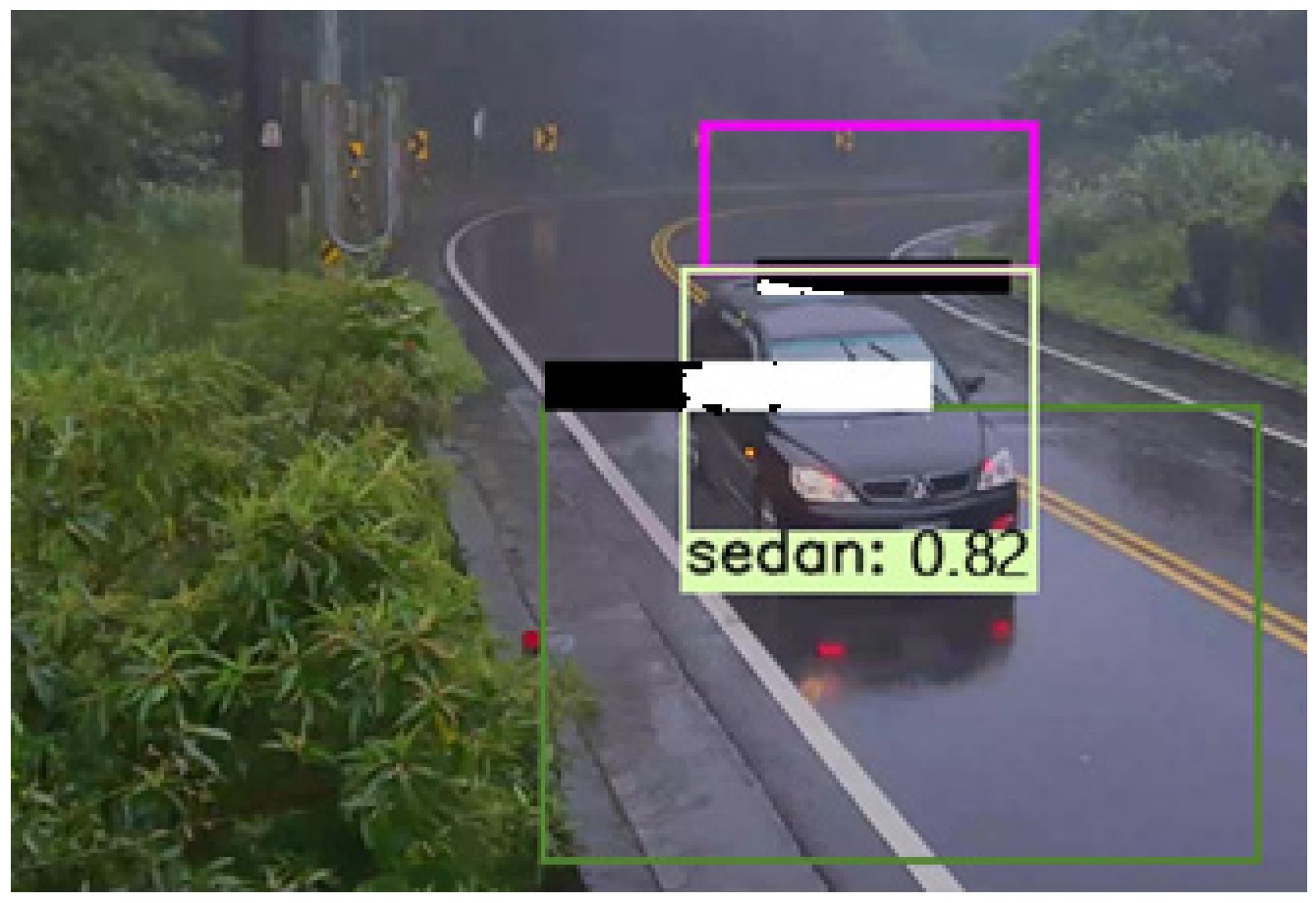
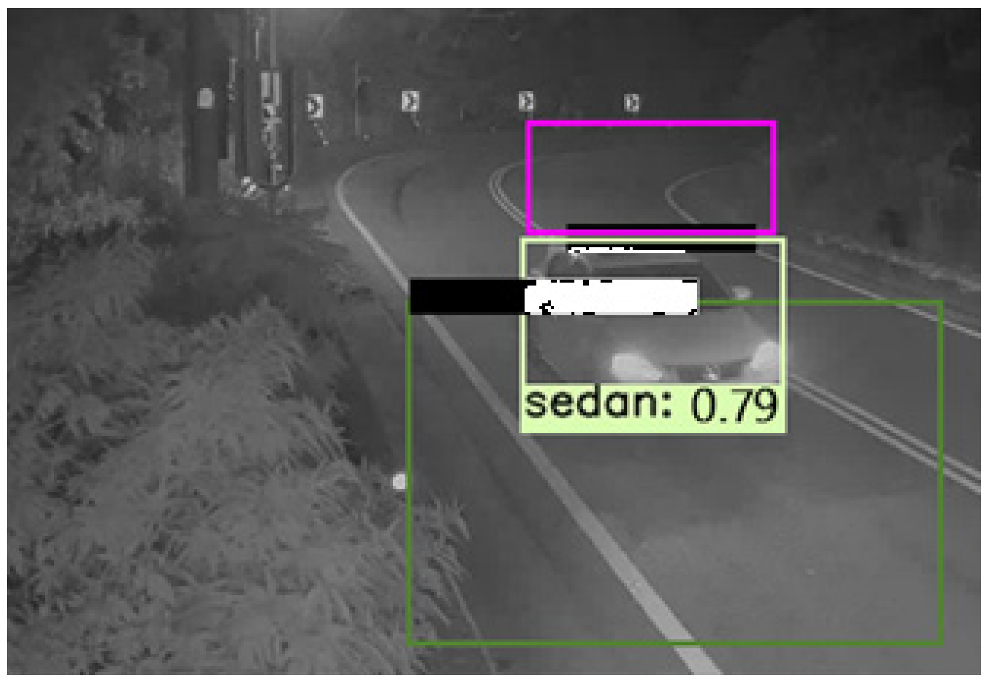
4.2. Detection Result at Different Weather Condition
5. Experiment and Results Comparison
Performance of the Test Datasets
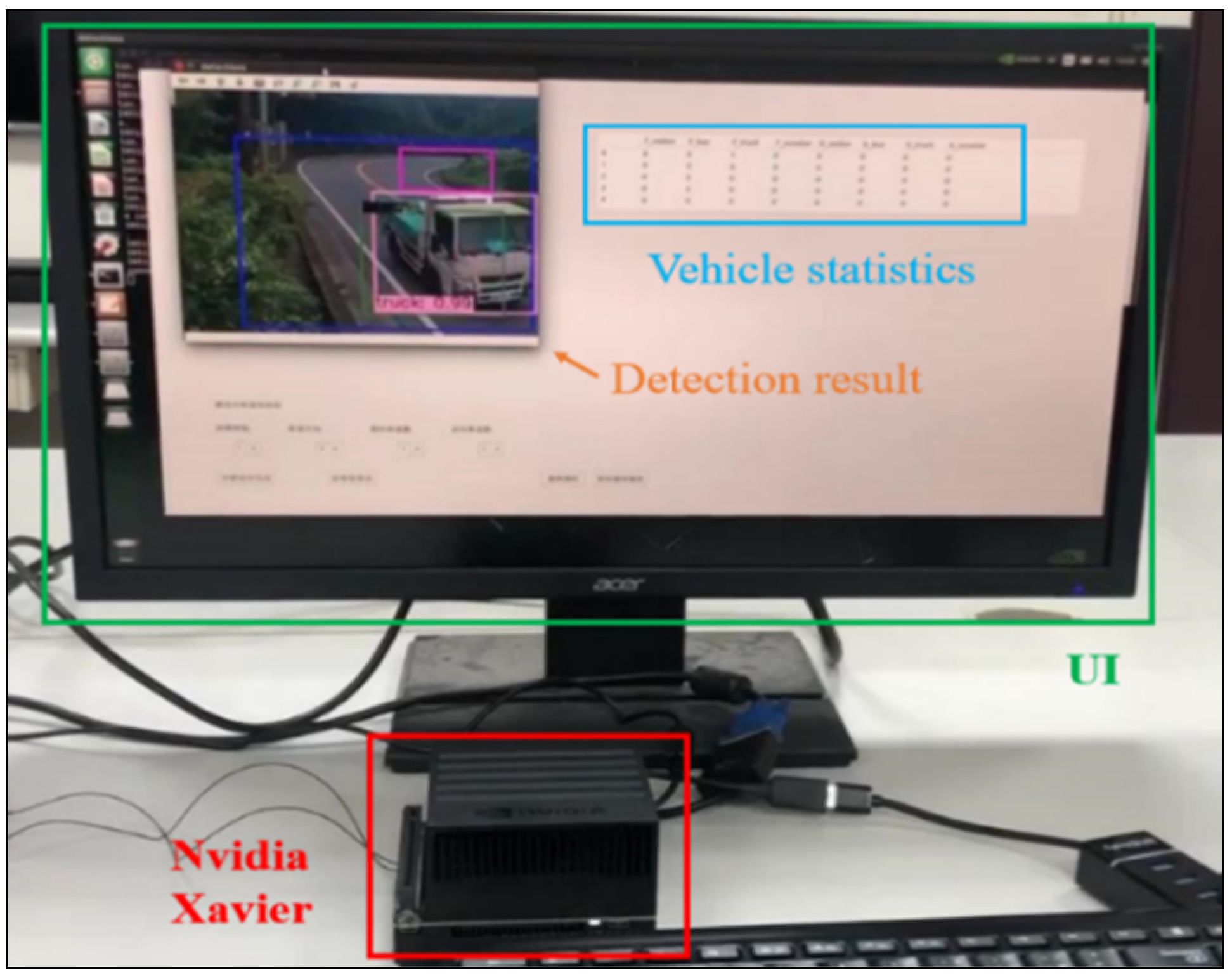
6. System Implementation
7. Discussion
8. Conclusions
Author Contributions
Funding
Institutional Review Board Statement
Informed Consent Statement
Data Availability Statement
Acknowledgments
Conflicts of Interest
References
- Ladislav, B.; Jaroslav, M. Changes in Road Traffic Caused by the Declaration of a State of Emergency in the Czech Republic—A Case Study. Transp. Res. Procedia 2021, 53, 321–328. [Google Scholar]
- Walid, B.; Hasan, T.; Hazem, H.R. Intelligent Vehicle Counting and Classification Sensor for Real-Time Traffic Surveillance. IEEE Trans. Intell. Transp. Syst. 2017, 19, 1789–1794. [Google Scholar]
- Cheng, H.Y.; Hsin, M.T. Vehicle Counting and Speed Estimation with RFID Backscatter Signal. In Proceedings of the IEEE Vehicular Networking Conference (VNC), Los Angeles, CA, USA, 4–6 December 2019; pp. 1–8. [Google Scholar]
- David, P.J.; David, S.K. An RFID-Enabled Road Pricing System for Transportation. IEEE Syst. J. 2008, 2, 248–257. [Google Scholar]
- Zhi, G.; Ruifang, Z.; Pengfei, W.; Xu, Y.; Hailong, Q.; Yazhe, T.; Bharath, R. Synergizing Appearance and Motion with Low-Rank Representation for Vehicle Counting and Traffic Flow Analysis. IEEE Trans. Intell. Transp. Syst. 2018, 19, 2675–2685. [Google Scholar]
- Honghong, Y.; Shiru, Q. Real-time Vehicle Detection and Counting in Complex Traffic Scenes Using Background Subtraction Model with Low-rank Decomposition. IET Intell. Transp. Syst. 2018, 12, 75–85. [Google Scholar]
- Lili, C.; Zhengdao, Z.; Li, P. Fast single-shot multi-box detector and its application on a vehicle counting system. IET Intell. Transp. Syst. 2018, 12, 1406–1413. [Google Scholar]
- Hou, X.; Zhang, L. Saliency Detection: A Spectral Residual Approach. In Proceedings of the IEEE Conference on Computer Vision and Pattern Recognition, Minneapolis, MN, USA, 17–22 June 2007; pp. 1–8. [Google Scholar]
- Yi, L.; Qiang, Z.; Dingwen, Z.; Jungong, H. Employing Deep Part-Object Relationships for Salient Object Detection. In Proceedings of the IEEE International Conference on Computer Vision (ICCV), Seoul, Korea, 27 October–2 November 2019; pp. 1232–1241. [Google Scholar]
- Dingwen, Z.; Haibin, T.; Jungong, H. Few-Cost Salient Object Detection with Adversarial-Paced Learning. In Proceedings of the 34th Conference on Neural Information Processing Systems (NeurIPS), Vancouver, BC, Canada, 6–12 December 2020; pp. 1–12. [Google Scholar]
- Dingwen, Z.; Junwei, H.; Yu, Z.; Dong, X. Synthesizing Supervision for Learning Deep Saliency Network without Human Annotation. IEEE Trans. Patte. Analy. Machi. Intell. 2020, 42, 1755–1769. [Google Scholar]
- Junwei, H.; Dingwen, Z.; Gong, C.; Nian, L.; Dong, X. Advanced Deep-Learning Techniques for Salient and Category-Specific Object Detection: A Survey. IEEE Signal Process. Magaz. 2018, 35, 84–100. [Google Scholar]
- Wen, L.; Dragomir, A.; Dumitru, E.; Christian, S.; Scott, R.; Cheng, Y.F.; Alexander, C.B. SSD: Single Shot MultiBox Detector. In Proceedings of the 14th European Conference, Amsterdam, The Netherlands, 11–14 October 2016; 2016; pp. 21–37. [Google Scholar]
- Christian, S.; Wei, L.; Yangqing, J.; Pierre, S.; Scott, R.; Dragomir, A.; Dumitru, E.; Vincent, V.; Andrew, R. Going Deeper with Convolutions. In Proceedings of the IEEE Conference on Computer Vision and Pattern Recognition (CVPR), Boston, MA, USA, 7–12 June 2015; pp. 1–9. [Google Scholar]
- Alex, K.; Ilya, S.; Geoffrey, E.H. ImageNet Classification with Deep Convolutional Neural Networks. In Proceedings of the 25th International Conference on Neural Information Processing Systems, Lake Tahoe, NV, USA, 3–6 December 2012; pp. 1097–1105. [Google Scholar]
- Mu, Y.; Brian, L.; Haoqiang, F.; Yuning, J. Randomized Spatial Pooling in Deep Convolutional Networks for Scene Recognition. In Proceedings of the IEEE International Conference on Image Processing (ICIP), Quebec City, QC, Canada, 27–30 September 2015; pp. 346–361. [Google Scholar]
- Ross, G.; Jeff, D.; Trevor, D.; Jitendra, M. Rich Feature Hierarchies for Accurate Object Detection and Semantic Segmentation. In Proceedings of the IEEE Conference on Computer Vision and Pattern Recognition, Columbus, OH, USA, 23–28 June 2014; pp. 580–587. [Google Scholar]
- Ross, G. Fast R-CNN. In Proceedings of the IEEE International Conference on Computer Vision (ICCV), Santiago, Chile, 7–13 December 2015; pp. 1440–1448. [Google Scholar]
- Shaoqing, R.; Kaiming, H.; Ross, G.; Jian, S. Faster R-CNN: Towards Real-time Object Detection with Region Proposal Networks. In Proceedings of the 28th International Conference on Neural Information Processing Systems, Montreal, QC, Canada, 7–12 December 2015; pp. 91–99. [Google Scholar]
- Kaiming, H.; Georgia, G.; Piotr, D.; Ross, G. Mask R-CNN. In Proceedings of the IEEE International Conference on Computer Vision (ICCV), Venice, Italy, 22–29 October 2017; pp. 2980–2988. [Google Scholar]
- Hyungtae, L.; Sungmin, E.; Heesung, K. ME R-CNN: Multi-Expert R-CNN for Object Detection. IEEE Trans. Image Process. 2020, 29, 1030–1044. [Google Scholar]
- Hui, Z.; Kunfeng, W.; Yonglin, T.; Chao, G.; Fei, Y.W. MFR-CNN: Incorporating Multi-Scale Features and Global Information for Traffic Object Detection. IEEE Trans. Vehicu. Techn. 2018, 67, 8019–8030. [Google Scholar]
- Hai, W.; Yijie, Y.; Yingfeng, C.; Xiaobo, C.; Long, C.; Yicheng, L. Soft-Weighted-Average Ensemble Vehicle Detection Method Based on Single-Stage and Two-Stage Deep Learning Models. IEEE Trans. Intell. Vehic. 2021, 6, 100–109. [Google Scholar]
- Yousong, Z.; Chaoyang, Z.; Haiyun, G.; Jinqiao, W.; Xu, Z.; Hanqing, L. Attention CoupleNet: Fully Convolutional Attention Coupling Network for Object Detection. IEEE Trans. Image Process. 2019, 28, 113–126. [Google Scholar]
- Joseph, R.; Santosh, D.; Ross, G.; Ali, F. You Only Look Once: Unified, Real-Time Object Detection. In Proceedings of the IEEE Conference on Computer Vision and Pattern Recognition (CVPR), Las Vegas, NV, USA, 27–30 June 2016; pp. 779–788. [Google Scholar]
- Zhishuai, Z.; Siyuan, Q.; Cihang, X.; Wei, S.; Bo, W.; Alan, L.Y. Single-Shot Object Detection with Enriched Semantics. In Proceedings of the IEEE Conference on Computer Vision and Pattern Recognition, Salt Lake City, UT, USA, 18–22 June 2018; pp. 5813–5821. [Google Scholar]
- Tsung, Y.L.; Priya, G.; Ross, G.; Kaiming, H.; Piotr, D. Focal Loss for Dense Object Detection. In Proceedings of the IEEE International Conference on Computer Vision (ICCV), Venice, Italy, 22–29 October 2017; pp. 2999–3007. [Google Scholar]
- Bichen, W.; Alvin, W.; Forrest, I.; Peter, H.J.; Kurt, K. SqueezeDet: Unified, Small, Low Power Fully Convolutional Neural Networks for Real-Time Object Detection for Autonomous Driving. In Proceedings of the IEEE Conference on Computer Vision and Pattern Recognition Workshops (CVPRW), Honolulu, HI, USA, 21–26 July 2017; pp. 446–454. [Google Scholar]
- Hei, L.; Jia, D. CornerNet: Detecting Objects as Paired Keypoints. In Proceedings of the 15th European Conference, Munich, Germany, 8–14 September 2018; pp. 765–781. [Google Scholar]
- Kaiyou, S.; Hua, Y.; Zhouping, Y. Multi-Scale Attention Deep Neural Network for Fast Accurate Object Detection. IEEE Trans. Circus. Syst. Video Techn. 2019, 29, 2972–2985. [Google Scholar]
- Seelam, S.K.; Voruganti, P.; Nandikonda, N.; Ramesh, T.K. Vehicle Detection Using Image Processing. In Proceedings of the IEEE International Conference for Innovation in Technology (INOCON), Bengaluru, India, 6–8 November 2020; pp. 1–5. [Google Scholar]
- Sheping, Z.; Dingrong, S.; Shuhuan, W.; Susu, D. DF-SSD: An Improved SSD Object Detection Algorithm Based on DenseNet and Feature Fusion. IEEE Access 2020, 8, 24344–24357. [Google Scholar]
- Palo, J.; Caban, J.; Kiktova, M.; Cernicky, L. The Comparison of Automatic Traffic Counting and Manual Traffic Counting. In Proceedings of the IOP Conference Series: Materials Science and Engineering; IOP Publishing: Bristol, UK, 2019. [Google Scholar] [CrossRef]
- Jie, H.; Li, S.; Gang, S. Squeeze-and-Excitation Networks. In Proceedings of the 2018 IEEE/CVF Conference on Computer Vision and Pattern Recognition, Salt Lake City, UT, USA, 18–23 June 2018; pp. 7132–7141. [Google Scholar]
- Lewis, F.L.; Liu, K. Towards a Paradigm for Fuzzy Logic Control. In Proceedings of the Industrial Fuzzy Control and Intellige (NAFIPS/IFIS/NASA ’94), San Antonio, TX, USA, 18–21 December 1994; pp. 94–100. [Google Scholar]
- Zadeh, L.A. Fuzzy sets. Inf. Control 1965, 8, 338–353. [Google Scholar] [CrossRef] [Green Version]
- Mark, E.; Luc, V.G.; Christopher, K.I.W.; John, W.; Andrew, Z. The PASCAL Visual Object Classes (VOC) Challenge. Int. J. Compu. Vis. 2010, 88, 303–338. [Google Scholar]
- Skala, H.J. Fuzzy Concepts: Logic, Motivation, Application. In Systems Theory in the Social Sciences; Birkhäuser: Basel, Switzerland, 1976; pp. 292–306. Available online: https://doi.org/10.1007/978-3-0348-5495-5_13 (accessed on 21 July 2021). [CrossRef]
- Timothy, J.R. Fuzzy Logic with Engineering Application, 3rd ed.; John Wiley & Sons Inc.: Hoboken, NJ, USA, 2010; pp. 90–94. [Google Scholar]
- Chris, S.; Grimson, W.E.L. Adaptive Background Mixture Models for Real-Time Tracking. In Proceedings of the IEEE Computer Society Conference on Computer Vision and Pattern Recognition, Fort Collins, CO, USA, 23–25 June 1999; pp. 246–256. [Google Scholar]
- Jiani, X.; Zhihui, W.; Daoerji, F. A Solution for Vehicle Attributes Recognition and Cross-dataset Annotation. In Proceedings of the 13th International Congress on Image and Signal Processing, BioMedical Engineering, and Informatics (CISP-BMEI), Chengdu, China, 17–19 October 2020; pp. 219–224. [Google Scholar]
- Yangqing, J.; Evan, S.; Jeff, D.; Sergey, K.; Jonathan, L.; Ross, G.; Sergio, G.; Trevor, D. Caffe: Convolutional Architecture for Fast Feature Embedding. In Proceedings of the 22nd ACM International Conference on Multimedia, New York, NY, USA, 3–7 November 2014; pp. 675–678. [Google Scholar]
- Zhe, D.; Huansheng, S.; Xuan, W.; Yong, F.; Xu, Y.; Zhaoyang, Z.; Huaiyu, L. Video-based Vehicle Counting Framework. IEEE Access 2019, 7, 64460–64470. [Google Scholar]
- Qi, C.M.; Hong, M.S.; Ling, Q.Z.; Rui, S.J. Finding Every Car: A Traffic Surveillance Multi-Scale Vehicle Object Detection Method. Appl. Intell. 2020, 50, 3125–3136. [Google Scholar]


| Model | Platform | FPS | Real-Time |
|---|---|---|---|
| ME R-CNN | GPU | 13.3 | No |
| MFR-CNN | GPU | 6.9 | No |
| A-Couple-Net | GPU | 9.5 | No |
| DF-SSD | GPU | 11.6 | No |
| YOLOv4 | Edge AI | 13.6 | No |
| SSD | Edge AI | 16.9 | No |
| b1 | b2 | b3 | b4 | b5 | b6 | b7 | b8 | b9 | b10 | b11 | b12 | b13 | ||
|---|---|---|---|---|---|---|---|---|---|---|---|---|---|---|
| s1 | fzy13 | fzy12 | fzy11 | fzy10 | fzy9 | fzy8 | fzy7 | fzy6 | fzy5 | fzy4 | fzy3 | fzy2 | fzy1 | |
| s2 | fzy12 | fzy12 | fzy11 | fzy10 | fzy9 | fzy8 | fzy7 | fzy6 | fzy5 | fzy4 | fzy3 | fzy2 | fzy1 | |
| s3 | fzy11 | fzy11 | fzy11 | fzy10 | fzy9 | fzy8 | fzy7 | fzy6 | fzy5 | fzy4 | fzy3 | fzy2 | fzy1 | |
| s4 | fzy10 | fzy10 | fzy10 | fzy10 | fzy9 | fzy8 | fzy7 | fzy6 | fzy5 | fzy4 | fzy3 | fzy2 | fzy1 | |
| s5 | fzy9 | fzy9 | fzy9 | fzy9 | fzy9 | fzy8 | fzy7 | fzy6 | fzy5 | fzy4 | fzy3 | fzy2 | fzy1 | |
| s6 | fzy8 | fzy8 | fzy8 | fzy8 | fzy8 | fzy8 | fzy7 | fzy6 | fzy5 | fzy4 | fzy3 | fzy2 | fzy1 | |
| s7 | fzy7 | fzy7 | fzy7 | fzy7 | fzy7 | fzy7 | fzy7 | fzy6 | fzy5 | fzy4 | fzy3 | fzy2 | fzy1 | |
| s8 | fzy6 | fzy6 | fzy6 | fzy6 | fzy6 | fzy6 | fzy6 | fzy6 | fzy5 | fzy4 | fzy3 | fzy2 | fzy1 | |
| s9 | fzy5 | fzy5 | fzy5 | fzy5 | fzy5 | fzy5 | fzy5 | fzy5 | fzy5 | fzy4 | fzy3 | fzy2 | fzy1 | |
| s10 | fzy4 | fzy4 | fzy4 | fzy4 | fzy4 | fzy4 | fzy4 | fzy4 | fzy4 | fzy4 | fzy3 | fzy2 | fzy1 | |
| s11 | fzy3 | fzy3 | fzy3 | fzy3 | fzy3 | fzy3 | fzy3 | fzy3 | fzy3 | fzy3 | fzy3 | fzy2 | fzy1 | |
| s12 | fzy2 | fzy2 | fzy2 | fzy2 | fzy2 | fzy2 | fzy2 | fzy2 | fzy2 | fzy2 | fzy2 | fzy2 | fzy1 | |
| s13 | fzy1 | fzy1 | fzy1 | fzy1 | fzy1 | fzy1 | fzy1 | fzy1 | fzy1 | fzy1 | fzy1 | fzy1 | fzy1 | |
| Model | Trainset | Jump-Threshold | mAP | FPS (PC) | FPS (Xavier) |
|---|---|---|---|---|---|
| FGSC-SSD | 07 + 12 | 0.08 | 74.0 | 60.6 | 19.1 |
| 07 + 12 | 0.1 | 74.1 | 63.4 | 19.6 | |
| 07 + 12 | 0.2 | 74.8 | 64.9 | 21.7 | |
| 07 + 12 | 0.3 | 73.2 | 65.2 | 20.4 |
| Block | The Ratio of Skipped Parameters |
|---|---|
| FGSC1 | 16/256 (6.2%) |
| FGSC2 | 258/512 (50.4%) |
| FGSC3 | 294/512 (57.4%) |
| FGSC4 | 541/1024 (53%) |
| FGSC5 | 276/512 (54%) |
| Method | Platform | mAP | FPS |
|---|---|---|---|
| ME R-CNN | Titan Xp | 72.2 | 13.3 |
| MSA-DNN | Titan Xp | 81.5 | 31.2 |
| SSD | Titan Xp | 81.7 | 31.5 |
| MFR-CNN | Titan X | 82.6 | 9.5 |
| DF-SSD | Titan X | 78.9 | 11.6 |
| ACoupleNet | Titan X | 83.1 | 6.9 |
| SSD | Titan X | 74.3 | 46 |
| YOLOv3 | 1080 Ti | 73.0 | 64.2 |
| YOLOv4 | 1080 Ti | 78.9 | 55.7 |
| SSD | 1080 Ti | 73.7 | 56 |
| FGSC-SSD | 1080 Ti | 73.8 | 64.9 |
| YOLOv3 | Xavier | 73.0 | 19.3 |
| YOLOv4 | Xavier | 78.9 | 13.6 |
| SSD | Xavier | 73.7 | 16.9 |
| FGSC-SSD | Xavier | 73.8 | 21.7 |
| Method | Platform | mAP | FPS |
|---|---|---|---|
| YOLOv3 | 1080 Ti | 96.3 | 26.2 |
| YOLOv4 | 1080 Ti | 95.1 | 25.3 |
| SSD | 1080 Ti | 91.4 | 23.9 |
| FGSC-SSD | 1080 Ti | 95.5 | 26.8 |
| YOLOv3 | Xavier | 96.3 | 20.2 |
| YOLOv4 | Xavier | 95.1 | 17.6 |
| SSD | Xavier | 91.4 | 15.4 |
| FGSC-SSD | Xavier | 95.5 | 21.7 |
| Method | Car | Bus | Truck | mAP |
|---|---|---|---|---|
| SSD | 86.8 | 85.3 | 85.1 | 85.7% |
| FGSC-SSD | 96.7 | 95.5 | 94.5 | 95.5% |
| Method | Platform | FPS (Video 640 × 480) |
|---|---|---|
| SSD | Xavier | 33.6 |
| FGSC-SSD | Xavier | 38.4 |
| Vehicle Types | Vehicle Numbers | Correctly Counting | Error Counting | Correctly Counted |
|---|---|---|---|---|
| Car | 61 | 59 | 2 | 96.7% |
| Bus | 44 | 42 | 2 | 95.5% |
| Truck | 36 | 34 | 2 | 94.5% |
Publisher’s Note: MDPI stays neutral with regard to jurisdictional claims in published maps and institutional affiliations. |
© 2021 by the authors. Licensee MDPI, Basel, Switzerland. This article is an open access article distributed under the terms and conditions of the Creative Commons Attribution (CC BY) license (https://creativecommons.org/licenses/by/4.0/).
Share and Cite
Sheu, M.-H.; Morsalin, S.M.S.; Zheng, J.-X.; Hsia, S.-C.; Lin, C.-J.; Chang, C.-Y. FGSC: Fuzzy Guided Scale Choice SSD Model for Edge AI Design on Real-Time Vehicle Detection and Class Counting. Sensors 2021, 21, 7399. https://doi.org/10.3390/s21217399
Sheu M-H, Morsalin SMS, Zheng J-X, Hsia S-C, Lin C-J, Chang C-Y. FGSC: Fuzzy Guided Scale Choice SSD Model for Edge AI Design on Real-Time Vehicle Detection and Class Counting. Sensors. 2021; 21(21):7399. https://doi.org/10.3390/s21217399
Chicago/Turabian StyleSheu, Ming-Hwa, S. M. Salahuddin Morsalin, Jia-Xiang Zheng, Shih-Chang Hsia, Cheng-Jian Lin, and Chuan-Yu Chang. 2021. "FGSC: Fuzzy Guided Scale Choice SSD Model for Edge AI Design on Real-Time Vehicle Detection and Class Counting" Sensors 21, no. 21: 7399. https://doi.org/10.3390/s21217399
APA StyleSheu, M.-H., Morsalin, S. M. S., Zheng, J.-X., Hsia, S.-C., Lin, C.-J., & Chang, C.-Y. (2021). FGSC: Fuzzy Guided Scale Choice SSD Model for Edge AI Design on Real-Time Vehicle Detection and Class Counting. Sensors, 21(21), 7399. https://doi.org/10.3390/s21217399