Figure 1.
U-map for iris data with the examples mapped as green, orange and blue dots.
Figure 1.
U-map for iris data with the examples mapped as green, orange and blue dots.
Figure 2.
U-images for example iris data. Each row contains three examples from a given class.
Figure 2.
U-images for example iris data. Each row contains three examples from a given class.
Figure 3.
Using U-images to train Convolutional Neural Network.
Figure 3.
Using U-images to train Convolutional Neural Network.
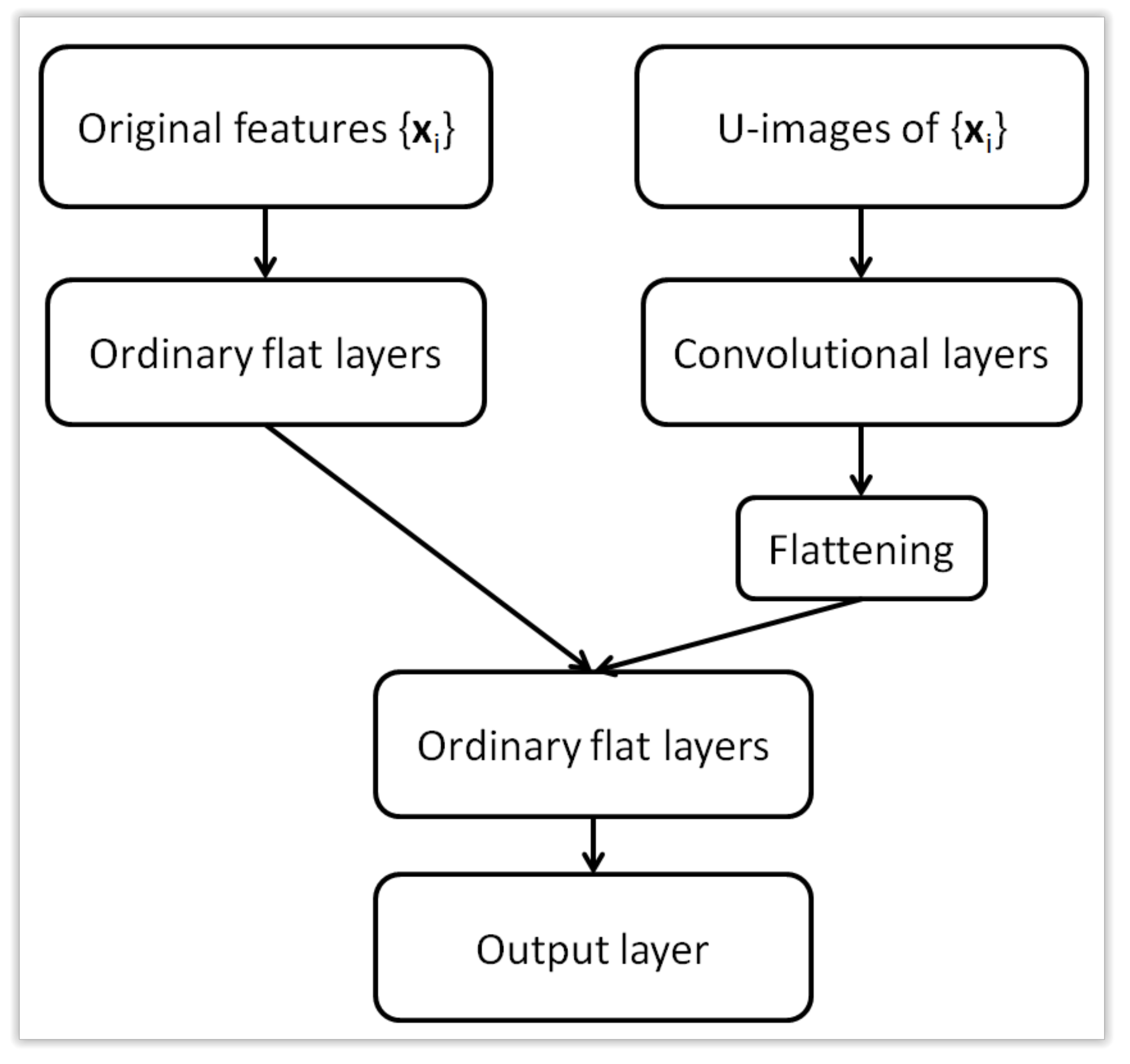
Figure 4.
Using both original data and U-images to train hybrid (multi-input) neural network with convolutional layers.
Figure 4.
Using both original data and U-images to train hybrid (multi-input) neural network with convolutional layers.
Figure 5.
Architecture of a hybrid (multi-input) neural network with two types of input data.
Figure 5.
Architecture of a hybrid (multi-input) neural network with two types of input data.
Figure 6.
Example architecture of an ordinary feed-forward neural network (the question mark represents the number of examples).
Figure 6.
Example architecture of an ordinary feed-forward neural network (the question mark represents the number of examples).
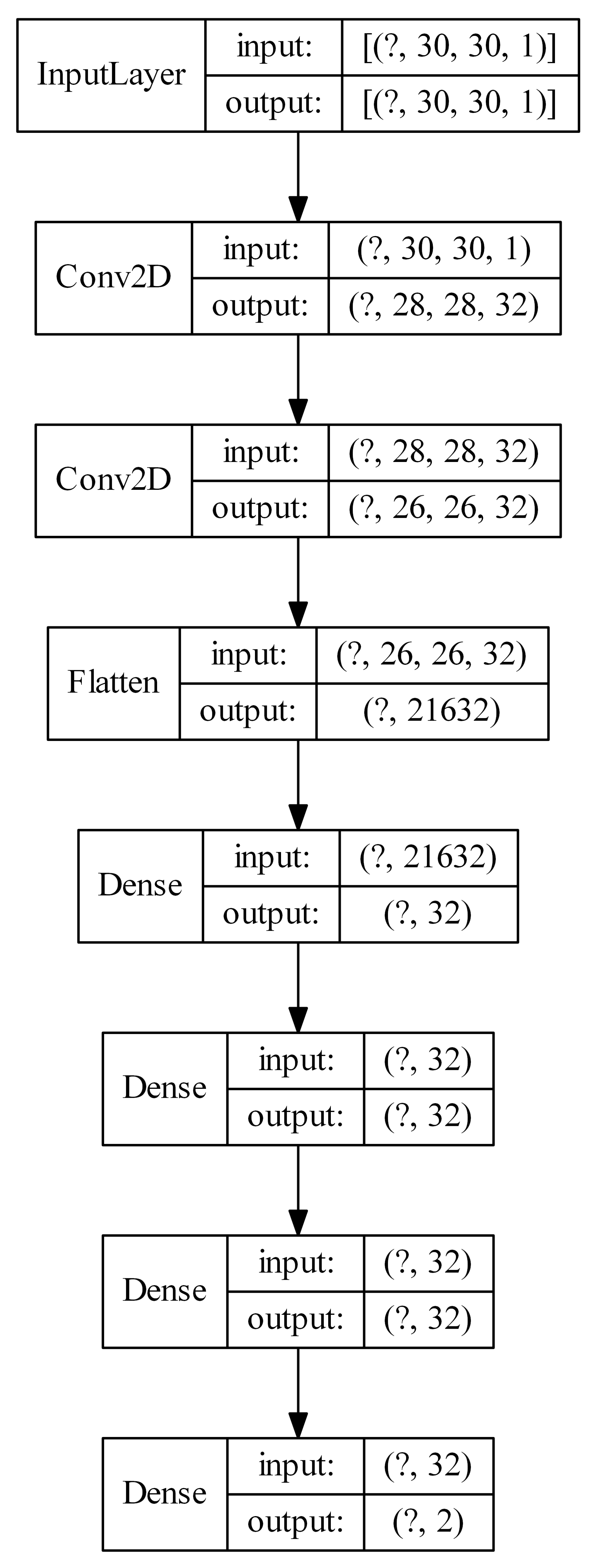
Figure 7.
Example architecture of a convolutional neural network with U-images produced by means of a Kohonen network as input (the question mark represents the number of examples).
Figure 7.
Example architecture of a convolutional neural network with U-images produced by means of a Kohonen network as input (the question mark represents the number of examples).
Figure 8.
Example architecture of a convolutional neural network with U-images as input, together with additional hidden flat layers (the question mark represents the number of examples).
Figure 8.
Example architecture of a convolutional neural network with U-images as input, together with additional hidden flat layers (the question mark represents the number of examples).
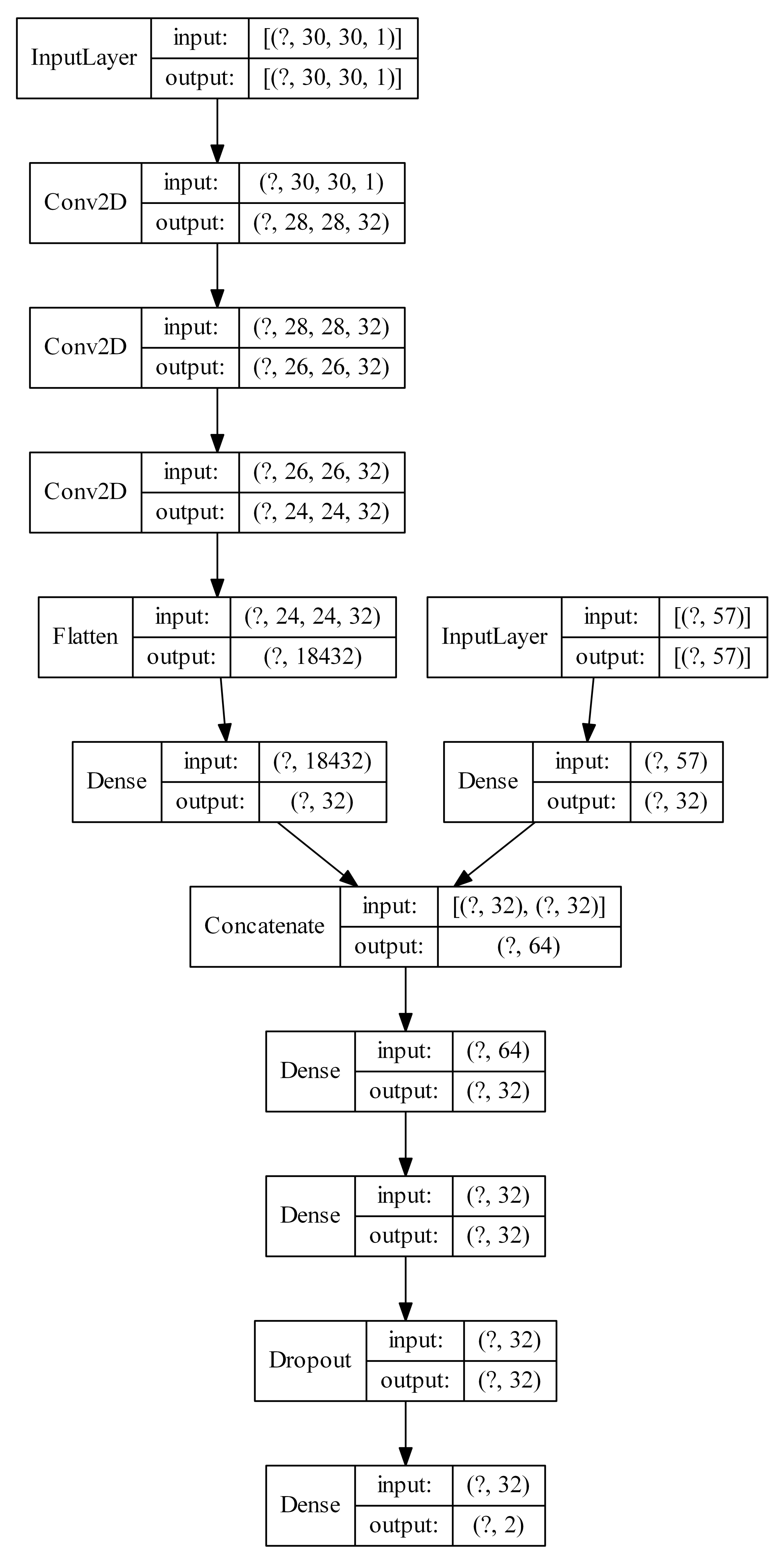
Figure 9.
Example architecture of a multiple input neural network (the question mark represents the number of examples).
Figure 9.
Example architecture of a multiple input neural network (the question mark represents the number of examples).
Figure 10.
Cross-validation test errors for different architectures for breast cancer wisconsin dataset.
Figure 10.
Cross-validation test errors for different architectures for breast cancer wisconsin dataset.
Figure 11.
Cross-validation test errors for different architectures for dataset 44 spambase.
Figure 11.
Cross-validation test errors for different architectures for dataset 44 spambase.
Figure 12.
Cross-validation test errors for different architectures for ILPD dataset.
Figure 12.
Cross-validation test errors for different architectures for ILPD dataset.
Figure 13.
Cross-validation test errors for different architectures for ionosphere dataset.
Figure 13.
Cross-validation test errors for different architectures for ionosphere dataset.
Figure 14.
Cross-validation test errors for different architectures for kc1 dataset.
Figure 14.
Cross-validation test errors for different architectures for kc1 dataset.
Figure 15.
Cross-validation test errors for different architectures for kc3 dataset.
Figure 15.
Cross-validation test errors for different architectures for kc3 dataset.
Figure 16.
Cross-validation test errors for different architectures for ozone-level-8hr dataset.
Figure 16.
Cross-validation test errors for different architectures for ozone-level-8hr dataset.
Figure 17.
Cross-validation test errors for different architectures for Parkinsons dataset.
Figure 17.
Cross-validation test errors for different architectures for Parkinsons dataset.
Figure 18.
Cross-validation test errors for different architectures for pima dataset.
Figure 18.
Cross-validation test errors for different architectures for pima dataset.
Figure 19.
Cross-validation test errors for different architectures for planning-relax dataset.
Figure 19.
Cross-validation test errors for different architectures for planning-relax dataset.
Figure 20.
Cross-validation test errors for different architectures for QSARbiodeg dataset.
Figure 20.
Cross-validation test errors for different architectures for QSARbiodeg dataset.
Figure 21.
Cross-validation test errors for different architectures for sonar dataset.
Figure 21.
Cross-validation test errors for different architectures for sonar dataset.
Figure 22.
Cross-validation test errors for different architectures for SPECTF dataset.
Figure 22.
Cross-validation test errors for different architectures for SPECTF dataset.
Figure 23.
Cross-validation test errors for different architectures for thoracic-surgery dataset.
Figure 23.
Cross-validation test errors for different architectures for thoracic-surgery dataset.
Figure 24.
Cross-validation test errors for different architectures for wisconsin diagnostic dataset.
Figure 24.
Cross-validation test errors for different architectures for wisconsin diagnostic dataset.
Figure 25.
Cross-validation test errors for different architectures for wisconsin prognostic dataset.
Figure 25.
Cross-validation test errors for different architectures for wisconsin prognostic dataset.
Table 1.
Machine learning test databases used in experiments.
Table 1.
Machine learning test databases used in experiments.
| No | Database | Examples | Features | Majority Class Ratio |
|---|
| 1 | breast cancer wisconsin | 683 | 9 | 0.6501 |
| 2 | dataset 44 spambase | 4601 | 57 | 0.6060 |
| 3 | ILPD | 579 | 10 | 0.7150 |
| 4 | ionosphere | 351 | 33 | 0.6410 |
| 5 | kc1 | 2109 | 21 | 0.8454 |
| 6 | kc3 | 458 | 39 | 0.9061 |
| 7 | ozone-level-8hr | 2534 | 72 | 0.9369 |
| 8 | parkinsons | 195 | 22 | 0.7538 |
| 9 | pima | 768 | 8 | 0.6510 |
| 10 | planning-relax | 182 | 12 | 0.7143 |
| 11 | QSARbiodeg | 1055 | 41 | 0.6626 |
| 12 | sonar | 208 | 60 | 0.5337 |
| 13 | SPECTF | 267 | 44 | 0.7940 |
| 14 | thoracic-surgery | 470 | 16 | 0.8511 |
| 15 | wisconsin diagnostic | 569 | 30 | 0.6274 |
| 16 | wisconsin prognostic | 194 | 32 | 0.7629 |
Table 2.
Results for ordinary feed-forward neural networks.
Table 2.
Results for ordinary feed-forward neural networks.
| No | Database | Mean Test Error [%] | StD [%] | Architecture |
|---|
| 1 | breast cancer wisconsin | 2.72 | 1.88 | 16-32 |
| 2 | dataset 44 spambase | 5.69 | 1.35 | 32 |
| 3 | ILPD | 28.11 | 9.26 | 32-32 |
| 4 | ionosphere | 5.85 | 3.54 | 16-32 |
| 5 | kc1 | 13.73 | 2.08 | 32-16-32 |
| 6 | kc3 | 8.36 | 3.90 | 16-16-32 |
| 7 | ozone-level-8hr | 5.62 | 1.45 | 16-32 |
| 8 | parkinsons | 13.63 | 6.82 | 32-32-32 |
| 9 | pima | 23.34 | 4.56 | 32 |
| 10 | planning-relax | 29.37 | 8.84 | 32 |
| 11 | QSARbiodeg | 12.19 | 2.62 | 16-16-32 |
| 12 | sonar | 13.45 | 6.02 | 32-16-32 |
| 13 | SPECTF | 18.93 | 10.31 | 32-32-32 |
| 14 | thoracic-surgery | 15.27 | 5.67 | 32-32 |
| 15 | wisconsin diagnostic | 2.87 | 1.44 | 32-32-32 |
| 16 | wisconsin prognostic | 23.48 | 13.12 | 32 |
Table 3.
Results for convolutional neural networks with inputs as U-images from Kohonen map.
Table 3.
Results for convolutional neural networks with inputs as U-images from Kohonen map.
| No | Database | Mean Test Error [%] | StD [%] | Architecture |
|---|
| 1 | breast cancer wisconsin | 2.74 | 1.88 | k20 × 20-cnn16 |
| 2 | dataset 44 spambase | 6.94 | 1.06 | k30 × 30-cnn32-16 |
| 3 | ILPD | 28.28 | 7.05 | k16 × 16-cnn16 |
| 4 | ionosphere | 3.80 | 3.08 | k30 × 30-cnn32-32 |
| 5 | kc1 | 14.29 | 1.96 | k20 × 20-cnn32-16 |
| 6 | kc3 | 8.97 | 4.46 | k20 × 20-cnn32-16 |
| 7 | ozone-level-8hr | 5.74 | 1.51 | k16 × 16-cnn32-16 |
| 8 | parkinsons | 8.61 | 3.70 | k30 × 30-cnn32-32 |
| 9 | pima | 22.76 | 4.60 | k16 × 16-cnn16 |
| 10 | planning-relax | 28.71 | 9.73 | k16 × 16-cnn16 |
| 11 | QSARbiodeg | 13.97 | 3.82 | k16 × 16-cnn32-16 |
| 12 | sonar | 16.03 | 5.47 | k30 × 30-cnn32-16 |
| 13 | SPECTF | 18.35 | 7.64 | k30 × 30-cnn32-16 |
| 14 | thoracic-surgery | 15.08 | 6.37 | k30 × 30-cnn32-32 |
| 15 | wisconsin diagnostic | 3.16 | 1.90 | k30 × 30-cnn32-32 |
| 16 | wisconsin prognostic | 23.85 | 12.73 | k24 × 24-cnn16 |
Table 4.
Results for convolutional neural networks with inputs as U-images from Kohonen map. Additional hidden flat layers were used.
Table 4.
Results for convolutional neural networks with inputs as U-images from Kohonen map. Additional hidden flat layers were used.
| No | Database | Mean Test Error [%] | StD [%] | Architecture |
|---|
| 1 | breast cancer wisconsin | 2.76 | 2.10 | k16 × 16-cnn16-nn32 |
| 2 | dataset 44 spambase | 7.00 | 0.62 | k20 × 20-cnn32-32-nn32 |
| 3 | ILPD | 28.12 | 6.96 | k16 × 16-cnn32-32-nn32-32 |
| 4 | ionosphere | 3.36 | 2.55 | k24 × 24-cnn32-32-nn32 |
| 5 | kc1 | 14.01 | 2.24 | k30 × 30-cnn16-nn32 |
| 6 | kc3 | 9.21 | 4.73 | k16 × 16-cnn16-nn32-32 |
| 7 | ozone-level-8hr | 5.56 | 1.30 | k16 × 16-cnn32-nn32 |
| 8 | parkinsons | 9.05 | 3.08 | k30 × 30-cnn32-32-nn32 |
| 9 | pima | 22.98 | 4.26 | k16 × 16-cnn16-nn32 |
| 10 | planning-relax | 29.85 | 9.51 | k16 × 16-cnn16-nn32 |
| 11 | QSARbiodeg | 13.12 | 2.49 | k30 × 30-cnn32-32-nn32-32 |
| 12 | sonar | 14.10 | 7.29 | k16 × 16-cnn32-32-nn32-32 |
| 13 | SPECTF | 16.24 | 8.47 | k20 × 20-cnn16-nn32 |
| 14 | thoracic-surgery | 15.09 | 6.22 | k24 × 24-cnn32-32-nn32 |
| 15 | wisconsin diagnostic | 2.63 | 1.54 | k24 × 24-cnn16-nn32 |
| 16 | wisconsin prognostic | 23.78 | 11.15 | k30 × 30-cnn32-nn32-32 |
Table 5.
Results for multiple input neural networks.
Table 5.
Results for multiple input neural networks.
| No | Database | Mean Test Error [%] | StD [%] | Architecture |
|---|
| 1 | breast cancer wisconsin | 2.92 | 1.93 | k24 × 24-1xconv-1 × 32-1 × 32 |
| 2 | dataset 44 spambase | 5.26 | 1.16 | k16 × 16-2xconv-1 × 32-1 × 32 |
| 3 | ILPD | 27.43 | 6.95 | k20 × 20-3xconv-1 × 32-2 × 32 |
| 4 | ionosphere | 3.64 | 3.45 | k30 × 30-2xconv-1 × 32-1 × 32 |
| 5 | kc1 | 14.36 | 1.91 | k16 × 16-1xconv-1 × 32-1 × 32 |
| 6 | kc3 | 9.18 | 4.67 | k16 × 16-1xconv-1 × 32-1 × 32 |
| 7 | ozone-level-8hr | 5.93 | 1.03 | k16 × 16-2xconv-1 × 32-2 × 32 |
| 8 | parkinsons | 7.21 | 4.37 | k30 × 30-2xconv-1 × 32-2 × 32 |
| 9 | pima | 24.33 | 5.36 | k20 × 20-2xconv-1 × 32-2 × 32 |
| 10 | planning-relax | 34.20 | 6.26 | k24 × 24-2xconv-1 × 32-1 × 32 |
| 11 | QSARbiodeg | 11.91 | 2.71 | k16 × 16-1xconv-1 × 32-1 × 32 |
| 12 | sonar | 11.28 | 7.22 | k24 × 24-3xconv-1 × 32-2 × 32 |
| 13 | SPECTF | 17.81 | 5.03 | k16 × 16-2xconv-1 × 32-2 × 32 |
| 14 | thoracic-surgery | 15.30 | 6.10 | k16 × 16-1xconv-1 × 32-1 × 32 |
| 15 | wisconsin diagnostic | 2.70 | 2.17 | k16 × 16-2xconv-1 × 32-1 × 32 |
| 16 | wisconsin prognostic | 23.81 | 12.28 | k24 × 24-1xconv-1 × 32-1 × 32 |
Table 6.
Summary of the results. Presented are mean test errors in %. Best results are underlined.
Table 6.
Summary of the results. Presented are mean test errors in %. Best results are underlined.
| No | Database | Ordinary NN | Kohonen-CNN | Hybrid | Multiple input |
|---|
| 1 | breast cancer wisconsin | 2.72 | 2.74 | 2.76 | 2.92 |
| 2 | dataset 44 spambase | 5.69 | 6.94 | 7.00 | 5.26 |
| 3 | ILPD | 28.11 | 28.28 | 28.12 | 27.43 |
| 4 | ionosphere | 5.85 | 3.80 | 3.36 | 3.64 |
| 5 | kc1 | 13.73 | 14.29 | 14.01 | 14.36 |
| 6 | kc3 | 8.36 | 8.97 | 9.21 | 9.18 |
| 7 | ozone-level-8hr | 5.62 | 5.74 | 5.56 | 5.93 |
| 8 | parkinsons | 13.63 | 8.61 | 9.05 | 7.21 |
| 9 | pima | 23.34 | 22.76 | 22.98 | 24.33 |
| 10 | planning-relax | 29.37 | 28.71 | 29.85 | 34.20 |
| 11 | QSARbiodeg | 12.19 | 13.97 | 13.12 | 11.91 |
| 12 | sonar | 13.45 | 16.03 | 14.10 | 11.28 |
| 13 | SPECTF | 18.93 | 18.35 | 16.24 | 17.81 |
| 14 | thoracic-surgery | 15.27 | 15.08 | 15.09 | 15.30 |
| 15 | wisconsin diagnostic | 2.87 | 3.16 | 2.63 | 2.70 |
| 16 | wisconsin prognostic | 23.48 | 23.85 | 23.78 | 23.81 |


