
Real-Time 2-D Lidar Odometry Based on ICP


Abstract
:1. Introduction
2. Related Work
3. System Overview
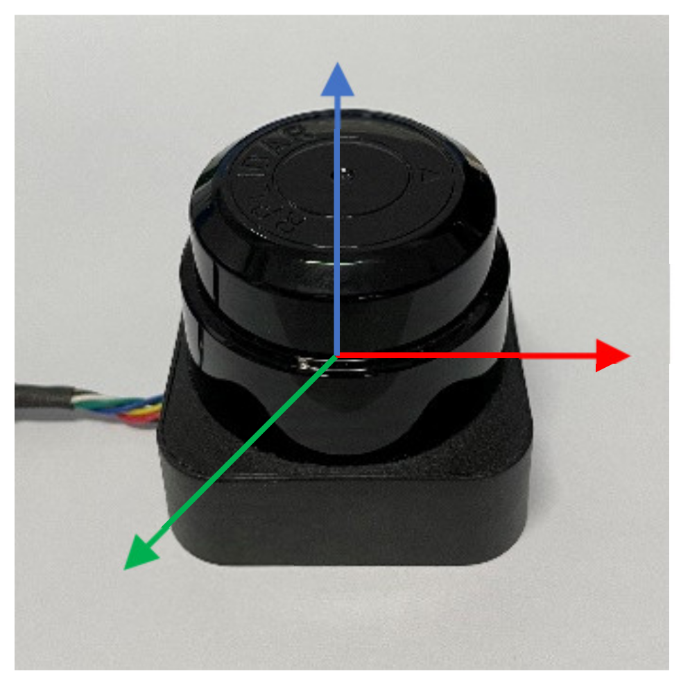
3.1. Lidar Hardware
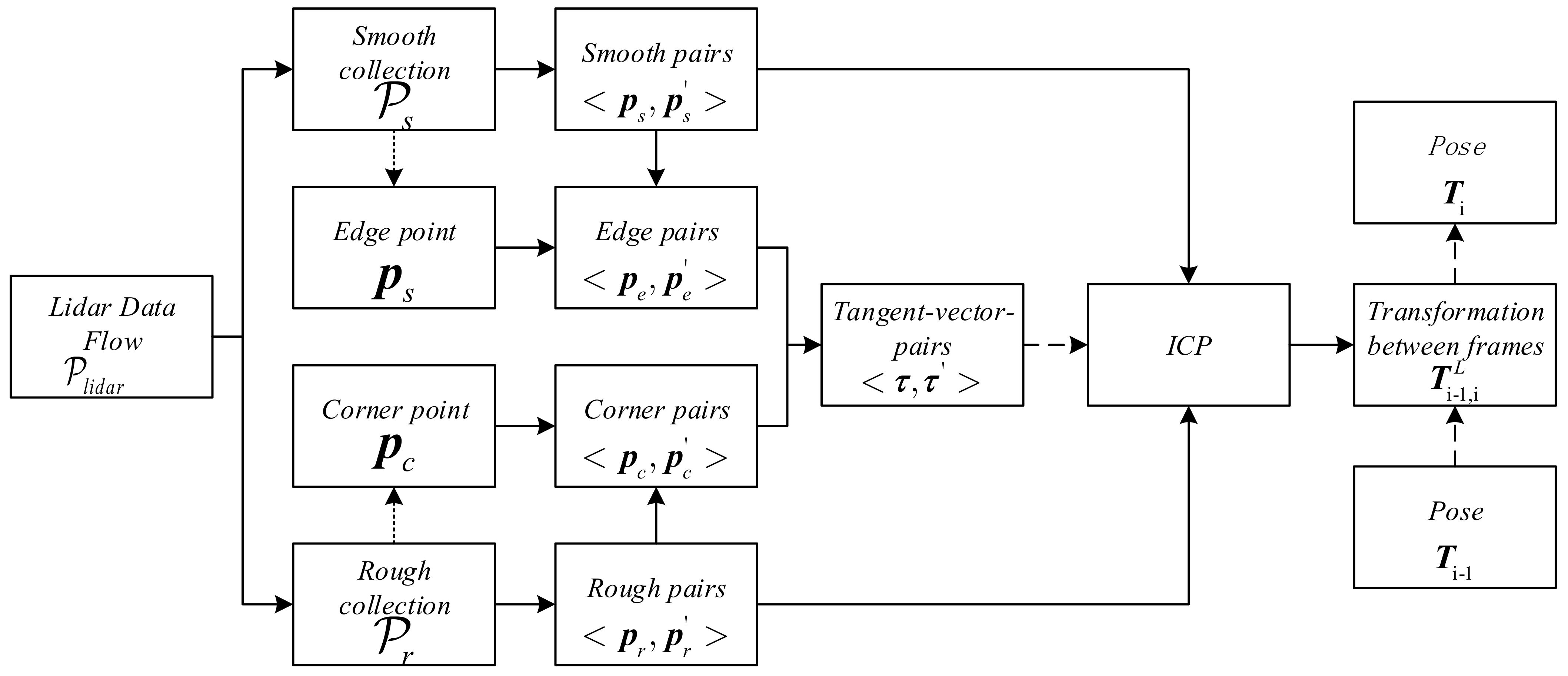
3.2. Software System Overview
4. Lidar Odometry
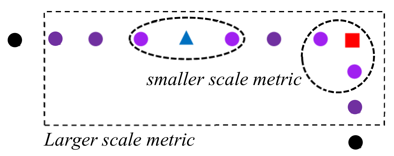
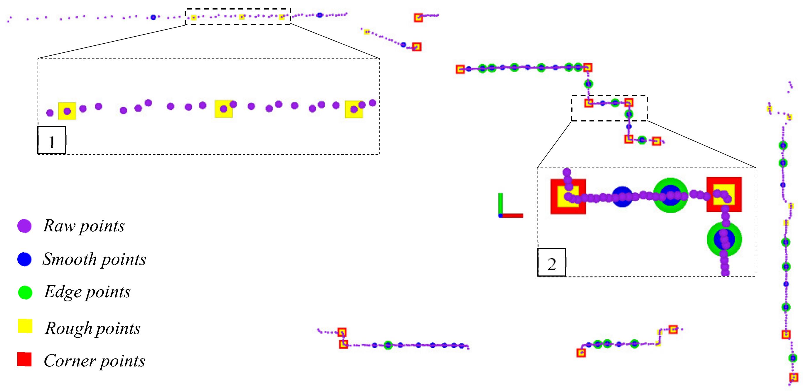
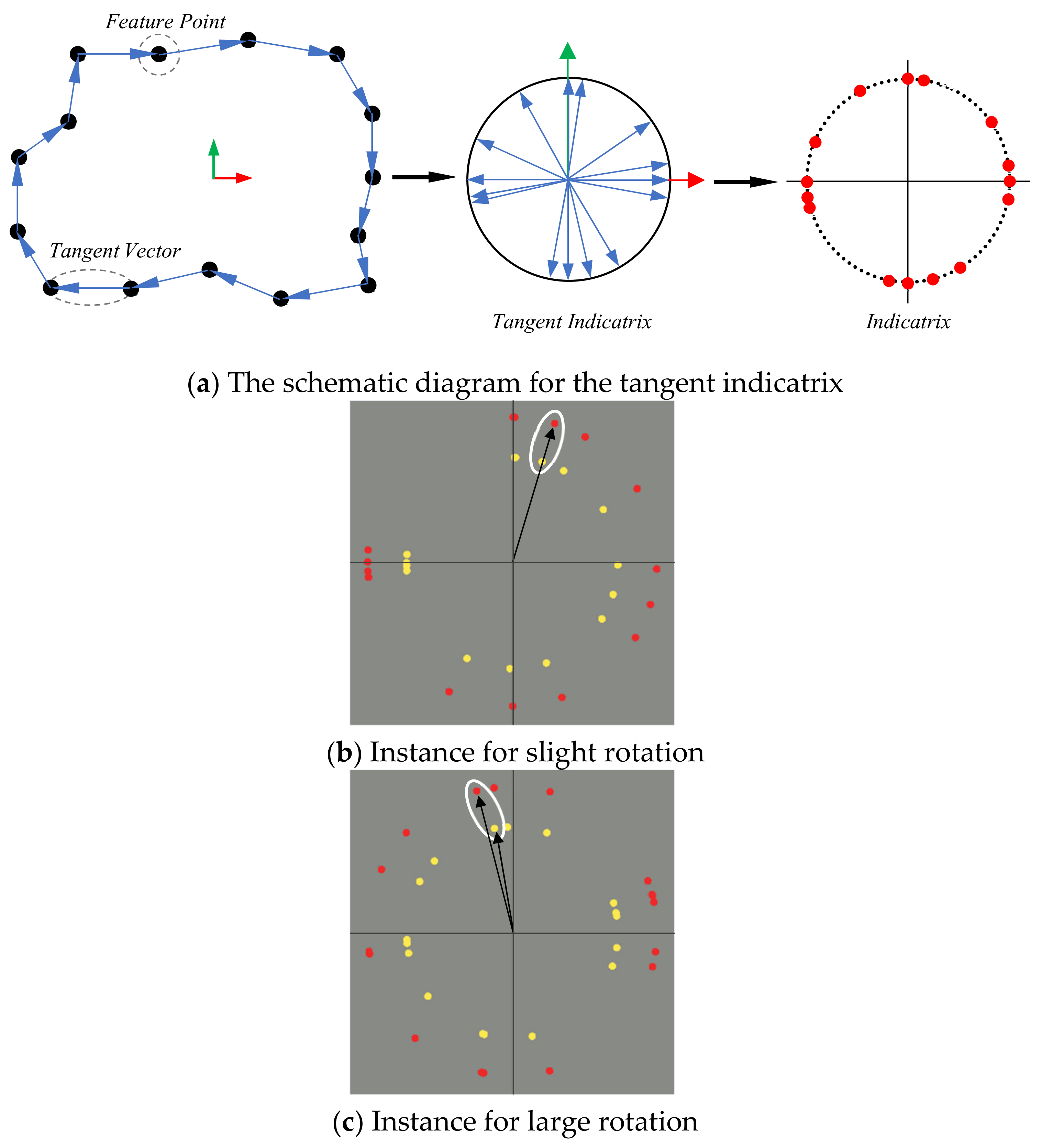
4.1. Feature Extraction
4.2. Motion Estimation
| Algorithm 1: Motion Estimation | |
| Input: smooth collection , rough collection | |
| Output: transformation matrix | |
| 1: | set to the identity matrix |
| 2: | for i = 0 to max iteration do |
| 3: | for each smooth point in or rough point in do |
| 4: | Find the closest point and for and in last scan regarding |
| to smooth collection and rough collection, respectively. | |
| 5: | All the point pairs and yield to Formula (5) |
| 6: | end for |
| 7: | Compute for all points in and . |
| 8: | for each point in and in do |
| 9: | Classify point as edge when and , |
| 10: | Classify point as corner when and . |
| 11: | All the point pairs and yield to Formulas (7) and (8). |
| 12: | end for |
| 13: | Compute new for all the points in and , |
| then obtain . | |
| 14: | Use and as input of Formula (6). |
| 15: | Use as input of Formula (10). |
| 16: | Update for next iteration. |
| 17: | if the convergence is satisfied then |
| 18: | Return |
| 19: | end if |
| 20: | end for |
5. Experiment
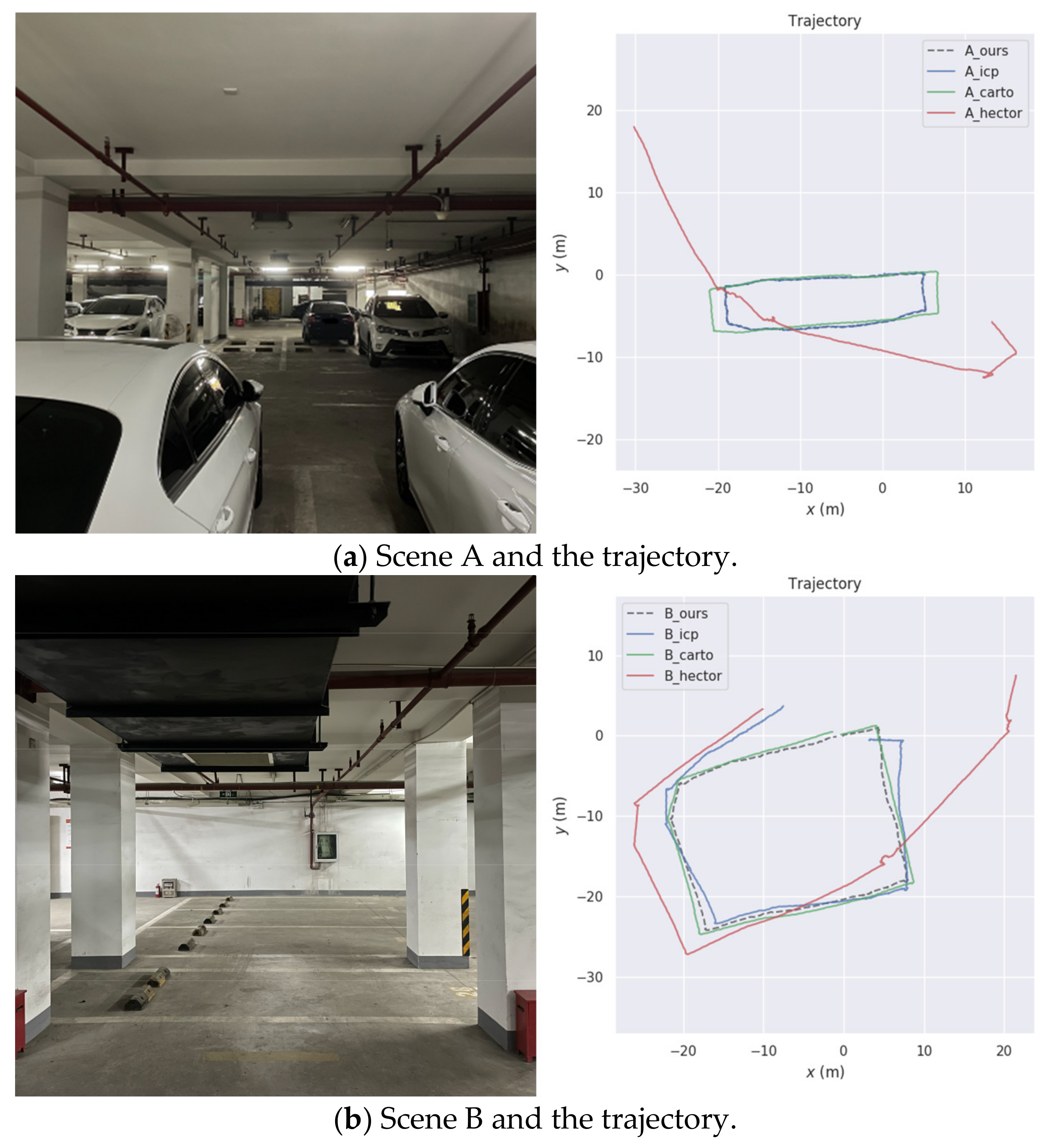
5.1. Our Datasets
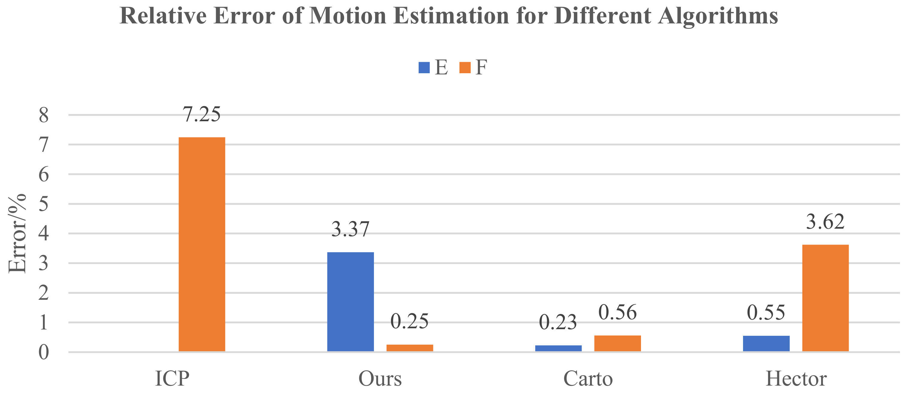
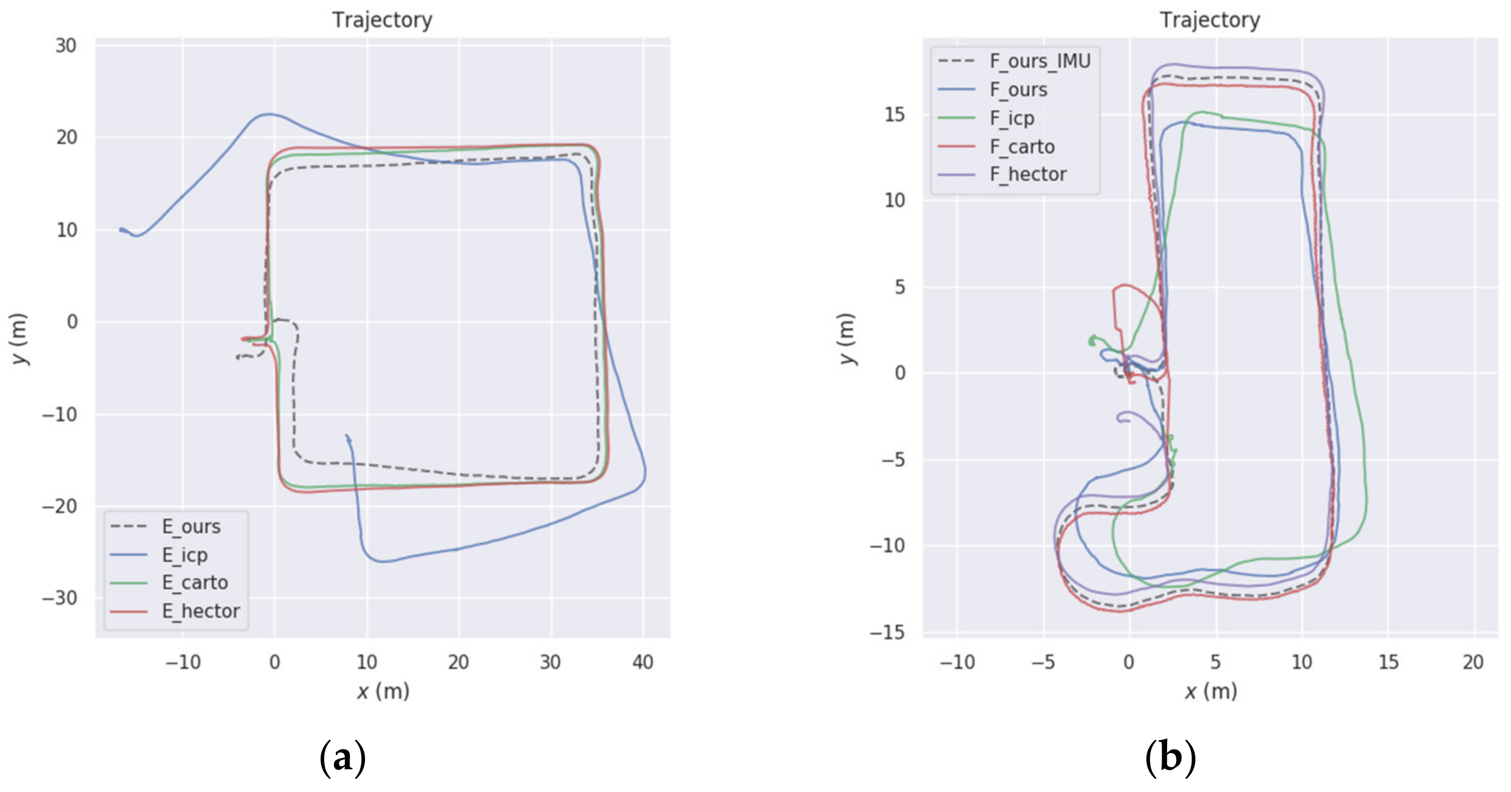
5.2. Open-Access Datasets
6. Conclusions
Author Contributions
Funding
Institutional Review Board Statement
Informed Consent Statement
Conflicts of Interest
References
- Liu, Q.; Liang, P.; Xia, J.; Wang, T.; Song, M.; Xu, X.; Zhang, J.; Fan, Y.; Liu, L. A Highly Accurate Positioning Solution for C-V2X Systems. Sensors 2021, 21, 1175. [Google Scholar] [CrossRef] [PubMed]
- Ilci, V.; Toth, C. High Definition 3D Map Creation Using GNSS/IMU/LiDAR Sensor Integration to Support Autonomous Vehicle Navigation. Sensors 2020, 20, 899. [Google Scholar] [CrossRef] [PubMed] [Green Version]
- Chiang, K.-W.; Tsai, G.-J.; Li, Y.-H.; Li, Y.; El-Sheimy, N. Navigation Engine Design for Automated Driving Using INS/GNSS/3D LiDAR-SLAM and Integrity Assessment. Remote Sens. 2020, 12, 1564. [Google Scholar] [CrossRef]
- Cadena, C.; Carlone, L.; Carrillo, H.; Latif, Y.; Scaramuzza, D.; Neira, J.; Reid, I.; Leonard, J.J. Past, Present, and Future of Simultaneous Localization and Mapping: Toward the Robust-Perception Age. IEEE Trans. Robot. 2016, 32, 1309–1332. [Google Scholar] [CrossRef] [Green Version]
- Su, T.; Zhu, H.; Zhao, P.; Li, Z.; Zhang, S.; Liang, H. A Robust LiDAR-based SLAM for Autonomous Vehicles aided by GPS/INS Integrated Navigation System. In Proceedings of the 2021 6th International Conference on Automation, Control and Robotics Engineering (CACRE), Dalian, China, 15–17 July 2021; pp. 351–358. [Google Scholar] [CrossRef]
- Thrun, S.; Burgard, W.; Fox, D. Probabilistic Robotics; The MIT Press: Cambridge, MA, USA, 2005. [Google Scholar]
- Konolige, K.; Grisetti, G.; Kümmerle, R.; Burgard, W.; Limketkai, B.; Vincent, R. Efficient Sparse Pose Adjustment for 2D mapping. In Proceedings of the 2010 IEEE/RSJ International Conference on Intelligent Robots and Systems, Taipei, Japan, 1–5 November 2010; pp. 22–29. [Google Scholar] [CrossRef] [Green Version]
- Kohlbrecher, S.; Von Stryk, O.; Meyer, J.; Klingauf, U. A flexible and scalable SLAM system with full 3D motion estimation. In Proceedings of the 2011 IEEE International Symposium on Safety, Security, and Rescue Robotics, Kyoto, Japan, 1–5 November 2011; pp. 155–160. [Google Scholar] [CrossRef] [Green Version]
- Durrant-Whyte, H.; Roy, N.; Pieter Abbeel, P. A Linear Approximation for Graph-Based Simultaneous Localization and Mapping. In Robotics: Science and Systems VII; MIT Press: Cambridge, MA, USA, 2012; pp. 41–48. [Google Scholar]
- Hess, W.; Kohler, D.; Rapp, H.; Andor, D. Real-time loop closure in 2D LIDAR SLAM. In Proceedings of the 2016 IEEE International Conference on Robotics and Automation (ICRA), Stockholm, Sweden, 16–21 May 2016; pp. 1271–1278. [Google Scholar] [CrossRef]
- Kümmerle, R.; Grisetti, G.; Strasdat, H.; Konolige, K.; Burgard, W. G2o: A general framework for graph optimization. In Proceedings of the 2011 IEEE International Conference on Robotics and Automation, Shanghai, China, 9–13 May 2011; pp. 3607–3613. [Google Scholar] [CrossRef]
- Besl, P.J.; McKay, N.D. A method for registration of 3-D shapes. IEEE Trans. Pattern Anal. Mach. Intell. 1992, 14, 239–256. [Google Scholar] [CrossRef]
- Censi, A. An ICP variant using a point-to-line metric. In Proceedings of the 2008 IEEE International Conference on Robotics and Automation, Pasadena, CA, USA, 19–23 May 2008; pp. 19–25. [Google Scholar] [CrossRef] [Green Version]
- Segal, A.; Haehnel, D.; Thrun, S. Generalized-ICP. Proc. Robot. Sci. Syst. 2009, 2, 435. [Google Scholar]
- Serafin, J.; Grisetti, G. NICP: Dense normal based point cloud registration. In Proceedings of the 2015 IEEE/RSJ International Conference on Intelligent Robots and Systems (IROS), Hamburg, Germany, 28 September–2 October 2015; pp. 742–749. [Google Scholar] [CrossRef] [Green Version]
- Deschaud, J.-E. IMLS-SLAM: Scan-to-model matching based on 3D data. Proc. IEEE Int. Conf. Robot. Automat. 2018, 2480–2485. [Google Scholar] [CrossRef] [Green Version]
- Tian, Y.; Liu, X.; Li, L.; Wang, W. Intensity-Assisted ICP for Fast Registration of 2D-LIDAR. Sensors 2019, 19, 2124. [Google Scholar] [CrossRef] [PubMed] [Green Version]
- Grisetti, G.; Stachniss, C.; Burgard, W. Improved Techniques for Grid Mapping with Rao-Blackwellized Particle Filters. IEEE Trans. Robot. 2007, 23, 34–46. [Google Scholar] [CrossRef] [Green Version]
- Steux, B.; El Hamzaoui, O. tinySLAM: A SLAM algorithm in less than 200 lines C-language program. In Proceedings of the 2010 11th International Conference on Control Automation Robotics & Vision, Singapore, 7–12 December 2010; pp. 1975–1979. [Google Scholar] [CrossRef]
- Ren, R.; Fu, H.; Wu, M. Large-Scale Outdoor SLAM Based on 2D Lidar. Electronics 2019, 8, 613. [Google Scholar] [CrossRef] [Green Version]
- Wen, J.; Qian, C.; Tang, J.; Liu, H.; Ye, W.; Fan, X. 2D LiDAR SLAM Back-End Optimization with Control Network Constraint for Mobile Mapping. Sensors 2018, 18, 3668. [Google Scholar] [CrossRef] [PubMed] [Green Version]
- Weichen, W.E.I.; Shirinzadeh, B.; Ghafarian, M.; Esakkiappan, S.; Shen, T. Hector SLAM with ICP Trajectory Matching. In Proceedings of the 2020 IEEE/ASME International Conference on Advanced Intelligent Mechatronics (AIM), Boston, MA, USA, 6–10 July 2020; pp. 1971–1976. [Google Scholar] [CrossRef]
- Zhang, J.; Singh, S. Low-drift and real-time lidar odometry and mapping. Auton. Robot. 2017, 41, 401–416. [Google Scholar] [CrossRef]
- Shan, T.; Englot, B. LeGO-LOAM: Lightweight and Ground-Optimized Lidar Odometry and Mapping on Variable Terrain. In Proceedings of the 2018 IEEE/RSJ International Conference on Intelligent Robots and Systems (IROS), Madrid, Spain, 1–5 October 2018; pp. 4758–4765. [Google Scholar] [CrossRef]
- Grant, W.S.; Voorhies, R.C.; Itti, L. Finding planes in LiDAR point clouds for real-time registration. In Proceedings of the 2013 IEEE/RSJ International Conference on Intelligent Robots and Systems, Tokyo, Japan, 3–7 November 2013; pp. 4347–4354. [Google Scholar] [CrossRef] [Green Version]
- Liu, Z.; Zhang, F. BALM: Bundle Adjustment for Lidar Mapping. IEEE Robot. Autom. Lett. 2021, 6, 3184–3191. [Google Scholar] [CrossRef]
- Zhou, L.; Koppel, D.; Kaess, M. LiDAR SLAM with Plane Adjustment for Indoor Environment. IEEE Robot. Autom. Lett. 2021, 6, 7073–7080. [Google Scholar] [CrossRef]
- Opromolla, R.; Fasano, G.; Grassi, M.; Savvaris, A.; Moccia, A. PCA-Based Line Detection from Range Data for Mapping and Localization-Aiding of UAVs. Int. J. Aerosp. Eng. 2017, 14. [Google Scholar] [CrossRef]
- Pfister, S.T.; Burdick, J.W. Multi-scale point and line range data algorithms for mapping and localization. In Proceedings of the 2006 IEEE International Conference on Robotics and Automation. ICRA 2006, Orlando, FL, USA, 15–19 May 2006; pp. 1159–1166. [Google Scholar] [CrossRef] [Green Version]
- Wu, D.; Meng, Y.; Zhan, K.; Ma, F. A LIDAR SLAM Based on Point-Line Features for Underground Mining Vehicle. In Proceedings of the 2018 Chinese Automation Congress (CAC), Xi’an, China, 30 November–2 December 2018; pp. 2879–2883. [Google Scholar] [CrossRef]
- Huang, R.; Hong, D.; Xu, Y.; Yao, W.; Stilla, U. Multi-Scale Local Context Embedding for LiDAR Point Cloud Classification. IEEE Geosci. Remote. Sens. Lett. 2020, 17, 721–725. [Google Scholar] [CrossRef]
- Bosse, M.; Zlot, R. Keypoint design and evaluation for place recognition in 2d lidar maps. Robot. Auton. Syst. 2009, 57, 1211–1224. [Google Scholar] [CrossRef]
- Lynen, S.; Achtelik, M.W.; Weiss, S.; Chli, M.; Siegwart, R. A robust and modular multi-sensor fusion approach applied to MAV navigation. In Proceedings of the 2013 IEEE/RSJ International Conference on Intelligent Robots and Systems, Tokyo, Japan, 3–7 November 2013; pp. 3923–3929. [Google Scholar] [CrossRef] [Green Version]
- Gao, Y.; Liu, S.; Atia, M.M.; Noureldin, A. INS/GPS/LiDAR Integrated Navigation System for Urban and Indoor Environments using Hybrid Scan Matching Algorithm. Sensors 2015, 15, 23286–23302. [Google Scholar] [CrossRef] [PubMed] [Green Version]
- Liu, S.; Martin, R.R.; Langbein, F.C.; Rosin, P.L. Segmenting Geometric Reliefs from Textured Background Surfaces. Comput.-Aided Des. Appl. 2007, 4, 565–583. [Google Scholar] [CrossRef]
- Grupp, M. Evo: Python Package for the Evaluation of Odometry and SLAM. 13 September 2017. Available online: https://github.com/MichaelGrupp/evo (accessed on 24 October 2021).


| Dataset | Time of Bag/s | Wall Clock Time/s | Real-Time |
|---|---|---|---|
| A | 192.5 | 67.2 | 2.9 |
| B | 245.3 | 145.4 | 1.7 |
| C | 134.3 | 75.1 | 1.8 |
| D | 81.9 | 47.9 | 1.7 |
| E | 145.4 | 129.2 | 1.1 |
| F | 105.2 | 89.6 | 1.2 |
| Module | Max (ms) | Min (ms) | Mean (ms) |
|---|---|---|---|
| Large-scale feature and data association | 89.3 | 10.7 | 56.1 |
| Small-scale feature and data association | 64.9 | 5.1 | 25.9 |
| Dataset | Error | Max/m | Min/m | Mean/m | RMSE/m |
|---|---|---|---|---|---|
| F | APE | 3.27 | 0.01 | 1.42 | 1.71 |
| RPE | 0.19 | <0.01 | 0.02 | 0.03 |
Publisher’s Note: MDPI stays neutral with regard to jurisdictional claims in published maps and institutional affiliations. |
© 2021 by the authors. Licensee MDPI, Basel, Switzerland. This article is an open access article distributed under the terms and conditions of the Creative Commons Attribution (CC BY) license (https://creativecommons.org/licenses/by/4.0/).
Share and Cite
Li, F.; Liu, S.; Zhao, X.; Zhang, L. Real-Time 2-D Lidar Odometry Based on ICP. Sensors 2021, 21, 7162. https://doi.org/10.3390/s21217162
Li F, Liu S, Zhao X, Zhang L. Real-Time 2-D Lidar Odometry Based on ICP. Sensors. 2021; 21(21):7162. https://doi.org/10.3390/s21217162
Chicago/Turabian StyleLi, Fuxing, Shenglan Liu, Xuedong Zhao, and Liyan Zhang. 2021. "Real-Time 2-D Lidar Odometry Based on ICP" Sensors 21, no. 21: 7162. https://doi.org/10.3390/s21217162
APA StyleLi, F., Liu, S., Zhao, X., & Zhang, L. (2021). Real-Time 2-D Lidar Odometry Based on ICP. Sensors, 21(21), 7162. https://doi.org/10.3390/s21217162