1. Introduction
Tens of billions of objects are connected to the 5G communication networks. These objects form the well-known Internet of Things (IoT), which is a promising application in future wireless networks [
1,
2,
3]. However, 5G IoT networks face serious challenges, which are caused by the complex, variable communication environment and big data produced. Therefore, the main issue is reducing energy consumption in 5G IoT networks. Compressive sensing (CS) [
4,
5,
6,
7,
8] presents some novel data-gathering strategies to reduce energy consumption in networks. According to the spatial, temporal, or spatial–temporal correlation characteristics of sensory data of 5G IoT networks, CS technique is able to recover the original senor node readings from
nodes with the help of
CS measurements as long as the signal can be sparsely represented in a certain transform domain [
9,
10]. CS is also capable of performing sensing and compression simultaneously to decrease transmission costs, aiming to save energy consumption for each node in the network.
A variety of compressive data-gathering schemes have been investigated for networks [
11,
12,
13,
14,
15,
16,
17,
18,
19,
20,
21,
22,
23,
24]. In reference [
11], sparsity in each of the decorrelated streams is used for temporal compression. In addition, the multivariate data are characterized using multivariate normal autoregression-integrated moving-average modeling before compression. Soheil Salehi et.al. proposed an adaptive compressed sampling via multi-bit crossbar array approach to intelligently generate the CS measurement matrix using a multi-bit STO-MRAM crossbar array. In addition, energy-aware adaptive sensing for IoT was introduced. It determined the frequency of measurement matrix updates within the energy budget of an IoT device. Qiao et al. proposed a media modulation-based mMTC (massive machine-type communication) solution for increasing the throughput. This technique leveraged the sparsity of the uplink access signals of mMTC received at the base station. A CS-based massive access solution was also promoted for tackling the challenge [
13]. In reference [
14], novel effective deterministic clustering using the CS technique was introduced to handle the data acquisition. Han et al. in reference [
15] proposed a multi-cluster cooperative CS scheme for large-scale IoT networks to observe physical quantities efficiently, which used cooperative observation and coherent transmission to realize CS measurement. However, existing sparse bases such as DCT (Discrete Cosine Transform), DFT (Discrete Fourier Transform) basis, and PCA (Principal Component Analysis) do not capture data structure characteristics in networks. As one of the statistical anomaly detection approaches, PCA can be applied to mark fraudulent transactions by evaluating applicable features to define what can be established as normal observation, and assign distance metrics to detect possible cases that serve as outliers/anomalies. However, it uses an orthogonal transformation of a set of observations of probably correlated variables into a set value of uncorrelated variables in a linear way. It serves a multivariate table as a smaller set of variables to be able to inspect trends, bounces, and outliers. In addition, the PCA method does not detect internal localized structures of original data. On the other hand, the PCA method does not provide multi-scale representation and eigenvalue analysis of data where the variables can occur in any given order. PCA achieves an optimal linear representation of the noisy data but is not necessary for noiseless observations in networks. It also does not gain multi-resolution representations. The proposed method in this paper has better performance in a noiseless environment for anomaly detection or outlier identification.
Some of the existing CS-based strategies try to exploit either spatial or temporal correlation of sensor node readings. Hence, the performance improvement brought by the CS approach is limited. Sensor node readings are generally periodically gathered for a long time. Therefore, the temporal correlation of each node can be further used. Additionally, sensor node readings have spatial correlation characteristics. Consequently, in this paper, spatial and temporal correlation features are both exploited to enhance data-gathering performance. As we know, for CS-based data-gathering methods, there are two important factors—sparse basis and measurement matrix—which should be considered. The measurement matrix includes the dense matrix [
10] and the sparse matrix [
24]. In reference [
10], Luo et al. provided a dense matrix, which satisfied RIP. Unfortunately, this type of matrix has high computational complexity, resulting in a high cost to transform network data. Therefore, Wang et al. presented a sparse random matrix, which demonstrated that this kind of matrix had optimal
-term approximation [
24]. Through many of experiments, Li et al. showed that recovery accuracy of sparse binary matrix outperformed existing sparse random matrixes [
25]. As a result, the sparse binary matrix was used to gather data and reconstruct original data.
Sparse representation of sensory data aims to achieve the sparsity basis of sensor node readings. In this paper, a spatial–temporal correlation basis algorithm (SCBA) of sensory data from the detected field will be constructed in detail. Zhao et al. first adopted the transform in [
26] to design a clustered compressive data aggregation scheme in networks [
27]. Unlike reference [
26], in this paper, according to sensory data characteristics, we design SCBA technology for 5G IoT networks. The optimal basis algorithm (OBA) is provided. At the end, we analyze the SCBA numerical sparsity using different sparsity metrics, and calculate the recovery error in view of different amounts of measurement combined with a sparse binary matrix.
The main contributions of this paper are as follows.
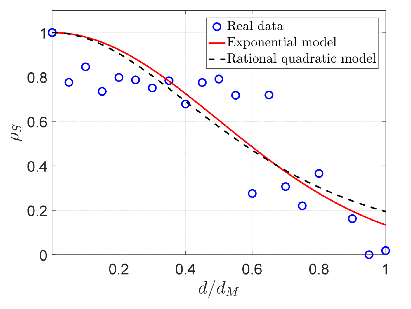
We analyze various real datasets of 5G IoT networks in terms of the exponential model and rational quadratic model, respectively. It shows that sensory data have high spatial–temporal correlation features.
In this paper, the SCBA method is put forward. In this algorithm, numerical sparsity is introduced to evaluate the performance of various sparse bases. In addition, algorithm complexity is also calculated. On the other hand, the OBA algorithm considering greedy scoring is presented. To compare the performance of the proposed SCBA with wavelet bases, the orthogonal wavelet basis algorithm (OWBA) is also presented.
We implement a variety of experiments based on real datasets of 5G IoT networks, including noiseless and noise environments. We compare our proposed SCBA with other sparse bases in view of different numerical sparsity and various recovery algorithms. Experiments demonstrate that the novel SCBA has better performance.
The rest of the paper is organized as follows.
Section 2 presents related work.
Section 3 provides CS backgrounds, the network model, and two different sparsity metrics. The spatial–temporal correlation properties of sensory data are analyzed though the power exponential (PE) model and the rational quadratic (RQ) model of networks, SCBA is constructed, and OBA is proposed in
Section 4.
Section 5 calculates the time complex of these proposed algorithms. In
Section 6, to verify the effectiveness of our presented algorithm, experiments on real datasets are carried out and related discussions are investigated. Conclusions and future work are given in
Section 7. A notation table is given in the
Table 1.
2. Related Work
Previous work related to sparse bases in networks can be sorted into the following four categories. The first is that they neither consider the spatial correlation nor consider the temporal correlation of sensory data in WSNs. For instance, DCT sparse basis [
19] was used and cost-aware stochastic compressive data-gathering was proposed. A Markov chain-based model was required to characterize the stochastic data-collection process. Sun et al. [
6] modeled the data loss induced by packet collisions and confirmed the corresponding compressive sensing projection matrix using the data loss pattern. Random sampling at each node was adopted and the optimal sensing probability was obtained. In the work in [
6], a DFT sparse basis was used to recovery original data. Ebrahimi et al. investigated the use of unmanned aerial vehicles (UAVs) for gathering data in networks [
22]. Projection-based compressive data-gathering (CDG) was attempted to aggregate sensory data. Projected nodes were chosen as cluster head nodes (CHs), while the UAV transferred that collected sensory data from the CHs to a distant sink node.
Another method is to only take into account the spatial correlation of sensory data. For example, Wu et al. [
28] proposed covariance-based sparse basis. The covariance matrix was defined as follows:
where
is a real symmetric matrix, and can be represented as
In reference [
28],
is used as a sparse basis.
A third is to only take into consideration the temporal correlation of sensory data. Wu et al. [
29] observed that the soil moisture process was relatively smooth and changed slowly, except at the onset of a rainfall. This technique tried to consider the difference between two adjacent sensory data samples, and the signal might be sparse represented. Therefore, the difference matrix was defined using Equation (3).
The fourth is to not only consider spatial correlation but also consider the temporal correlation of sensory data. Chen et al. provided a Fréchet mean estimate sparse basis [
30]. In this work, both the intra-sensor and inter-sensor correlation were exploited to decrease the number of samples required for recovering of the original sensory data. It depicts that spatial and temporal correlation of a signal are considered simultaneously. Moreover, a Fréchet mean enhanced the greedy algorithm, called precognition matching pursuit (PMP). Quer et al. [
31] investigated the problem of compressing a large and distributed signal of networks and reconstructed it though a small number of samples. Bayesian analysis was proposed to approximate the statistical distribution of the principal components, and to demonstrate that the Laplacian distribution provided a precise representation of the statistics of original sensory data. Principal Component Analysis (PCA) was exploited to capture not only the spatial but also the temporal correlation features of real data. In reference [
32], covariogram-based compressive sensing (CBCS) was presented. In particular, Kronecker CS framework was employed to leverage the spatial–temporal correlation characteristics. CBCS performance showed that it was superior to DFT, distributed source coding, etc. It was also able to adapt efficiently and promptly to change for the signal.
Motivated by the fourth type of sparse representation basis, this paper produces SCBA aiming for the sparest representation of the sensory data in 5G IoT networks such that there is a reduction in energy consumption.
4. Algorithm Details
Sparsest bases play an important role in the compressive data-gathering technique of networks. DCT, wavelet basis, and the PCA algorithm are widely used in conventional compressive data-gathering schemes. Unfortunately, these existing sparse bases do not capture intrinsic features of a signal. Take PCA, for example. PCA can obtain a global representation, where each basis vector is a linear combination of all the original data. It is not easy to detect internal localized structures of original data. On the other hand, the PCA method does not provide multi-scale representation and eigenvalue analysis of data where variables can occur in any given order. In addition, PCA achieves an optimal linear representation of noisy data but is not necessary for noiseless observations in networks. Therefore, when the number of observations is far greater than the number of variables, the principal elements may be interfered with by the noise. IoT networks fall into this category. In other words, the number of sensor node observations is no less than the amount of sensor nodes in the networks. Thus, in this paper, motivated by hierarchical clustering tree and wavelets [
25], a novel algorithm that not only captures localized data structure characteristics, but also gains multi-resolution representations, is presented. SCBA is summarized in Algorithm 1.
In Algorithm 1, there are three stages that include the calculation of the two most similar sum variables, building a hierarchical tree of 2 × 2 Jacobi rotations and constructing a basis for the Jacobi tree Algorithms.
Stage1: For this algorithm, in step 1, covariance matrix
is the general covariance, which is shown in Equation (12). The correlation coefficients
is described using Equation (13), and the similarity matrix is represented as Equation (14).
where
. Subsequently, in step 2, we calculate the most similar sum variables based on the similarity matrix
. However, at the initial stage 1, when input dataset is
, for instance, the size of an extracted matrix from the temperature of the DEI-Campaign A is
. If we calculate correlation coefficients between different rows for each column vector, it means that the spatial correlation is considered. When we calculate correlation coefficients between different columns for each row vector, it shows that the temporal correlation is also taken into account. In application, for a detected environment of 5G IoT networks, we choose datasets as input variables
of several minutes frame length which are enough to explore the intrinsic features of sensor node readings. By means of these collected data, we can design a SCBA schedule. Consequently, in the following compressive data-gathering scheme, we can combine the measurement matrix with the given reconstruction algorithm to recover the original signals in the sink node of networks.
Stage2: Steps 3–24 mainly construct a tree of Jacobi rotations. In step 4, variable is applied to store Jacobi rotations matrix, while denotes rotation angle. Variable is the order of the principle component. Next, Step 7 initializes the related parameters of the algorithm. For the loop, steps 8–24 calculate Jacobi rotations for each level of the tree. Variable and represent covariance matrix and the correlation coefficient matrix , respectively. By naming the function, we accomplish a change of basis and new coordinates, which corresponds to steps 9–15. Steps 16–23 reveal various approaches of variable storage. Step 16 is the number of new variables for sum and difference components. and represent the position of the 1st and the 2nd principal components at step 17, respectively. So far, it has constructed a Jacobi tree.
Stage3: Then, in the following steps, we will produce the orthogonal basis for the aforementioned Jacobi tree algorithm. The loop of 26–34 is the core of the orthogonal basis algorithm, which repeats until achieves the maximum . However, denotes a 2 × 2 rotation matrix. The two principal components and are stored in variables and , respectively, that correspond to lines 29–33. It is worth stressing that is the fraction of basis functions of subspaces , and is the basis functions of subspaces . In addition, the spatial–temporal correlation basis algorithm is similar to standard multi-resolution analysis: The SCBA algorithm provides a set of “scale functions”. Those functions are defined on subspaces and a group of orthogonal functions are defined on residual subspaces , where such that they achieve a multi-resolution transformation. Thus, the orthogonal basis is the concatenation of and (lines 35–39).
However, in Algorithm 1, the default basis selection is the maximum-height tree. The choice results in a fully parameter-free decomposition of the original data. In addition, it is also specifically for the idea of a multi-scale analysis. In practice, for a compressive data-gathering technique for 5G IoT networks, we alternatively select any of the orthogonal bases at various levels of the tree. The algorithm provides an approach that is inspired by the idea in reference [
45]. We assume that the original data
is a
-dimensional random vector. We suppose that the candidate orthogonal bases are
, where
denotes the basis at level
of the tree. Subsequently, we find the best sparse representation for the original signal. Here, in Algorithm 2, scoring criteria are applied to measure the percentage of explained variance for the selected coordinates. Consequently, greedy scoring and choice method is presented in the following Equation (15).
where for an orthogonal basis
, each vector
is assigned an energy score based on the above Equation (15). Therefore, the optimal basis is the basis with the highest energy score. In Algorithm 2, line 3 describes the value of the molecule, and line 5 represents the value of the denominator of
. Of course, in Algorithm 2, the other two sparsity measurement strategies are taken to evaluate the performance of the spatial–temporal correlation sparse basis. Line 6 and line 7 are 1-norm and 2-norm, respectively. They are used to compute GI and NS, respectively, and steps 10–11 of Algorithm 2 are the GI index and NS evaluation approaches. Then, line 12 arranges the energy score in Equation (15) in descending order such that we find the best orthogonal basis with the maximum energy score. At the end, lines 13–16 obtain the optimal basis. In addition, the flow chart of SCBA is shown in
Figure 4. The main steps of SCBA input the needed parameters, calculating the two most similar sum variables, building a hierarchical tree of 2 by 2 Jacobi rotations and constructing a basis for the Jacobi tree algorithm.
| Algorithm 1 The spatial–temporal correlation basis algorithm with highly efficient (SCBA) |
| Input:, , (total number of observations), , |
| Output: return an orthogonal basis |
| % calculate the two most similar sum variables |
| 1: calculate covariance matrix , correlation coefficients , similarity matrix |
| 2: obtain the two most similar sum variables based on |
| % build a hierarchical tree of 2 by 2 Jacobi rotations |
| 3: |
| 4: |
| 5: |
| 6: |
| 7: initialization |
| 8: for |
| 9: |
| 10: |
| 11: |
| 12: |
| 13: |
| 14: |
| 15: , |
| 16: |
| 17: , |
| 18: |
| 19. |
| 20. |
| 21: |
| 22: |
| 23: |
| 24: end |
| % construct basis for the Jacobi tree algorithm |
| 25: , |
| 26: for |
| 27: |
| 28: |
| 29: |
| 30: |
| 31: |
| 32: |
| 33: |
| 34: end |
| 35: if nargin < 4 |
| 36: |
| 37: else |
| 38: |
| 39: end |
| Algorithm 2 optimal basis algorithm with greedy scoring (OBA) |
| Input:, |
| Output: the best Treelet orthogonal basis: |
| 1: calculate |
| 2: |
| 3: |
| 4:if |
| 5: |
| 6: |
| 7: |
| 8: end |
| 9: |
| 10: calculate index using Equation (4) |
| 11: calculate by using Equation (5) |
| 12: |
| 13: if |
| 14: |
| 15: end |
| 16: |
To demonstrate the efficiency of SCBA, in
Section 6, we perform plenty of comparison experiments including spatial, DCT, haar-1, haar-2, and rbio5.5 bases. However, since the standard wavelet algorithm is not an orthogonal basis, Algorithm 3 proposes the OWBA scheme with a similar idea in reference [
47]. In Algorithm 3, step 1 takes the rbio5.5 algorithm, for example, by means of filtering, and decomposes out the high and low filter coefficients. Line 2 calculates the length of the filter, and line 3 and line 4 obtain the maximum and minimum of the observation vectors, respectively. Step 5 is the initialization of the wavelet orthogonal basis. The loop of steps 6–18 aims to construct the orthogonal matrix. It is noted that the length of the signal is the integer power of 2 that is shown in step 7. Hence, in the subsequent experiment, the frame lengths of data on rbio5.5 and haar are chosen as the integer power of 2. Lines 8–9 construct two vectors. Nevertheless, in the coming loop, the aforementioned vector in lines 8–9 is circle-shifted (step 10–13). Finally, we generate the orthogonal matrix, namely the wavelet orthogonal basis
(lines 14–17). As a result, OWBA returns an orthogonal basis until the variable
achieves the maximum, i.e.,
.
| Algorithm 3 orthogonal wavelet basis algorithm (OWBA) |
| Input: original data , measurement size , (frame length of data), sparsity |
| Output: wavelet orthogonal basis: |
| 1. |
| 2. |
| 3. |
| 4. |
| 5. |
| 6. for |
| 7. |
| 8. |
| 9. |
| 10. for |
| 11. |
| 12. |
| 13. end |
| 14. |
| 15. |
| 16. |
| 17. |
| 18. end |


