
Dual Crisscross Attention Module for Road Extraction from Remote Sensing Images

Abstract
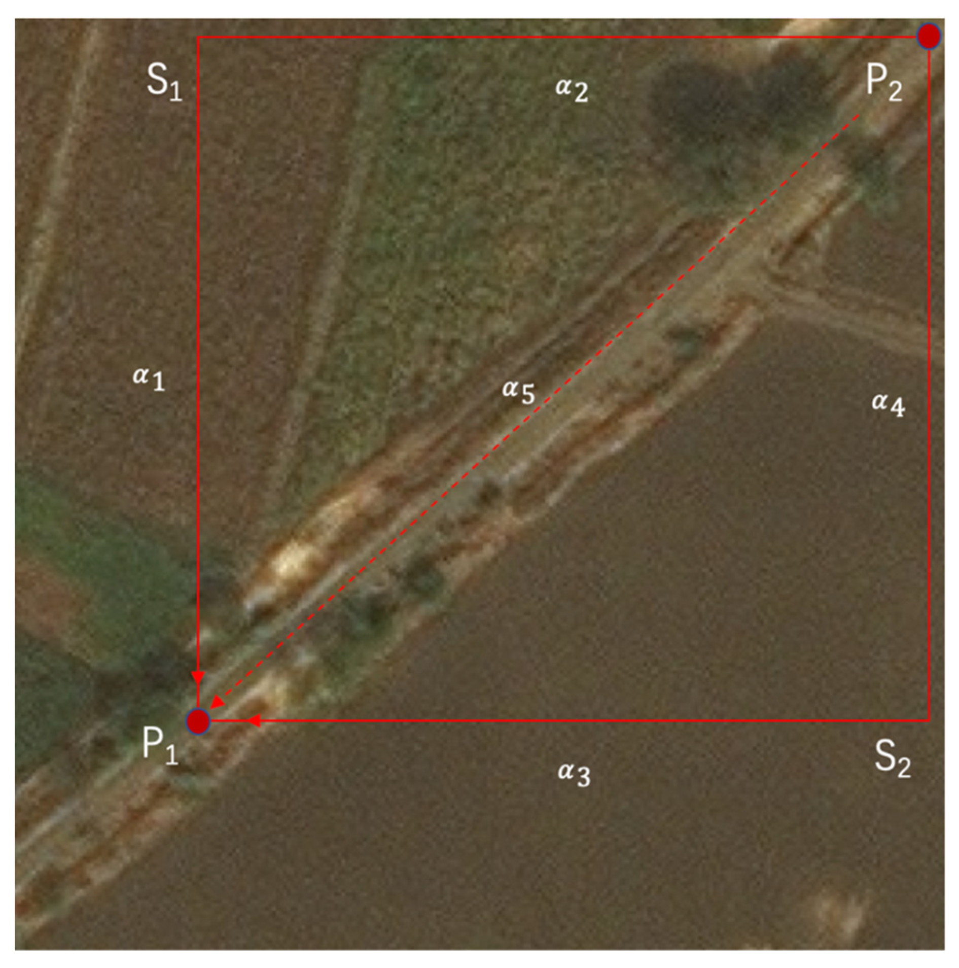
:1. Introduction
2. Related Work
2.1. Semantic Segmentation Based on Deep Learning
2.2. Attention Mechanism and Its Implementation in CNN
2.3. Attention Mechanism and Its Implementation in CNN
3. Methodology
3.1. Framework
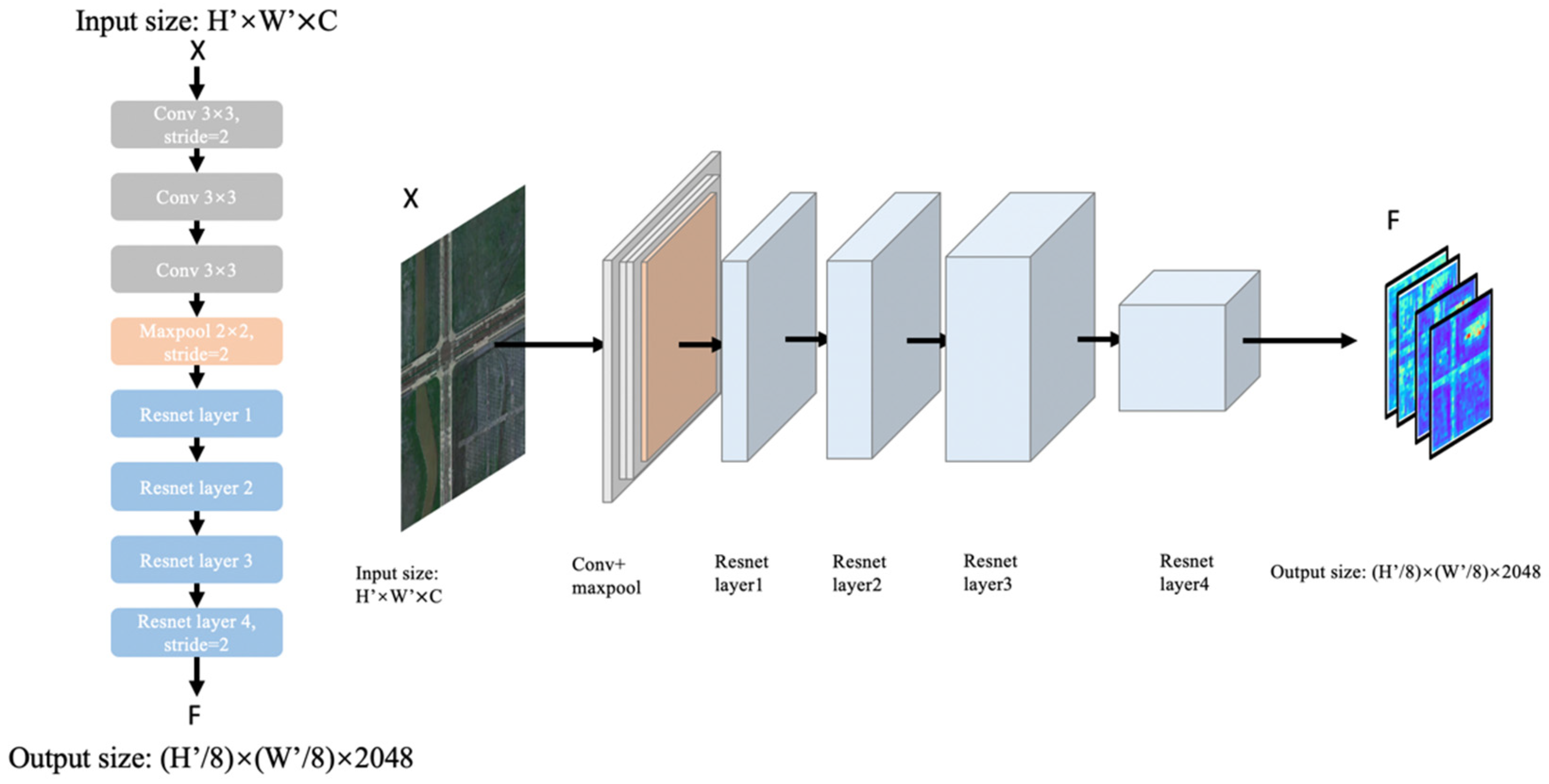
3.1.1. Backbone
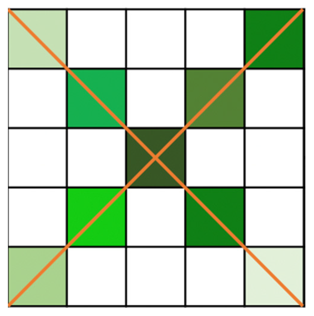
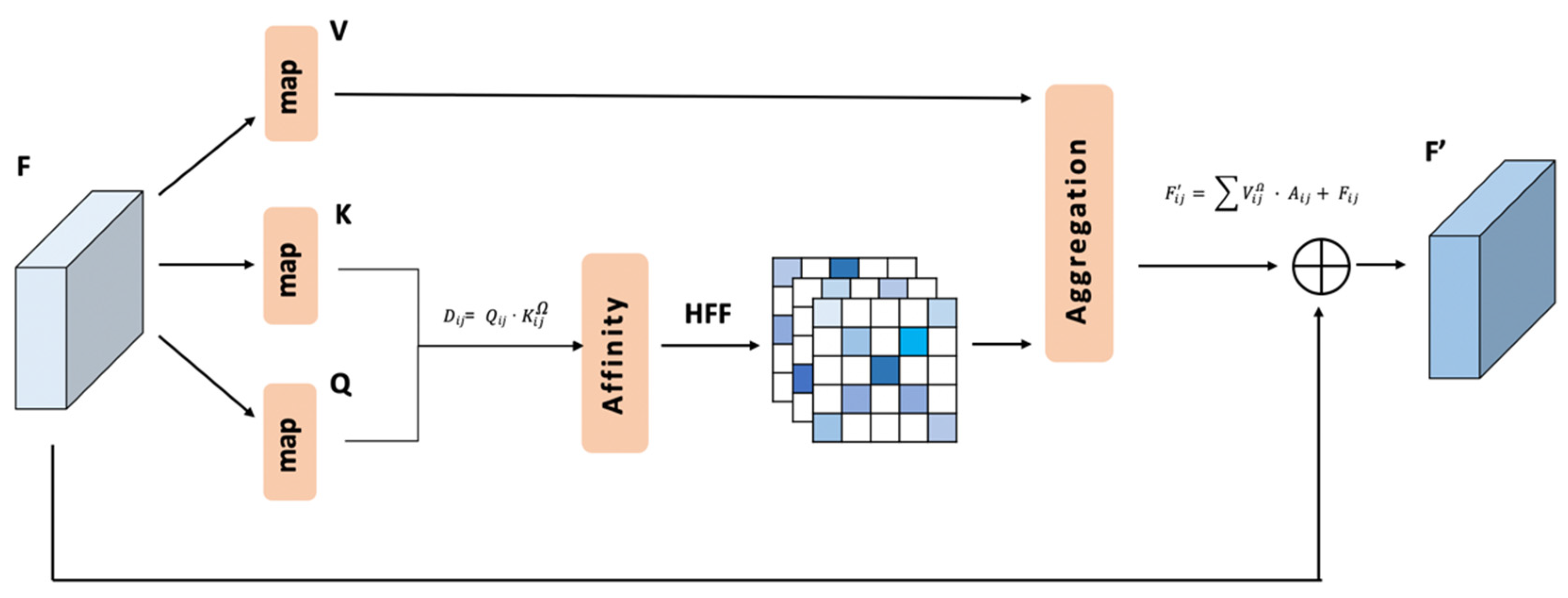
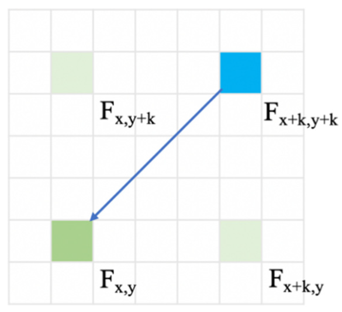
3.1.2. The Implementation of CCA Module
3.2. Introduction of the RCCA Module
3.2.1. Design and Realization of the RCCA Module
| Algorithm 1. The process of RCCA attention. |
1: 2: /* According to the points groups () and (, get feature value of the RCCA region positions in K. */ /* and represent the range of index on the horizontal axis of the feature map. */ 3: 4: 5: 6: 7: 8: 9: 10: /* represents the channel vectors sets of the RCCA region in K. */ 11: /* Search Q corresponding to the position in K and then get the energy map E */ 12: 13: 14: /* Apply activation function HFF to the energy map, HFF is defined in 3.3 */ 15: 16: 17: /* According to the point set () and (, get feature value of RCCA region positions in V */ 18: /* Aggregate E and V and represents the residual structure */ 19: 20: 21: |
3.2.2. Functional Merits of the RCCA Module
3.2.3. Computational Advantages of the RCCA Module
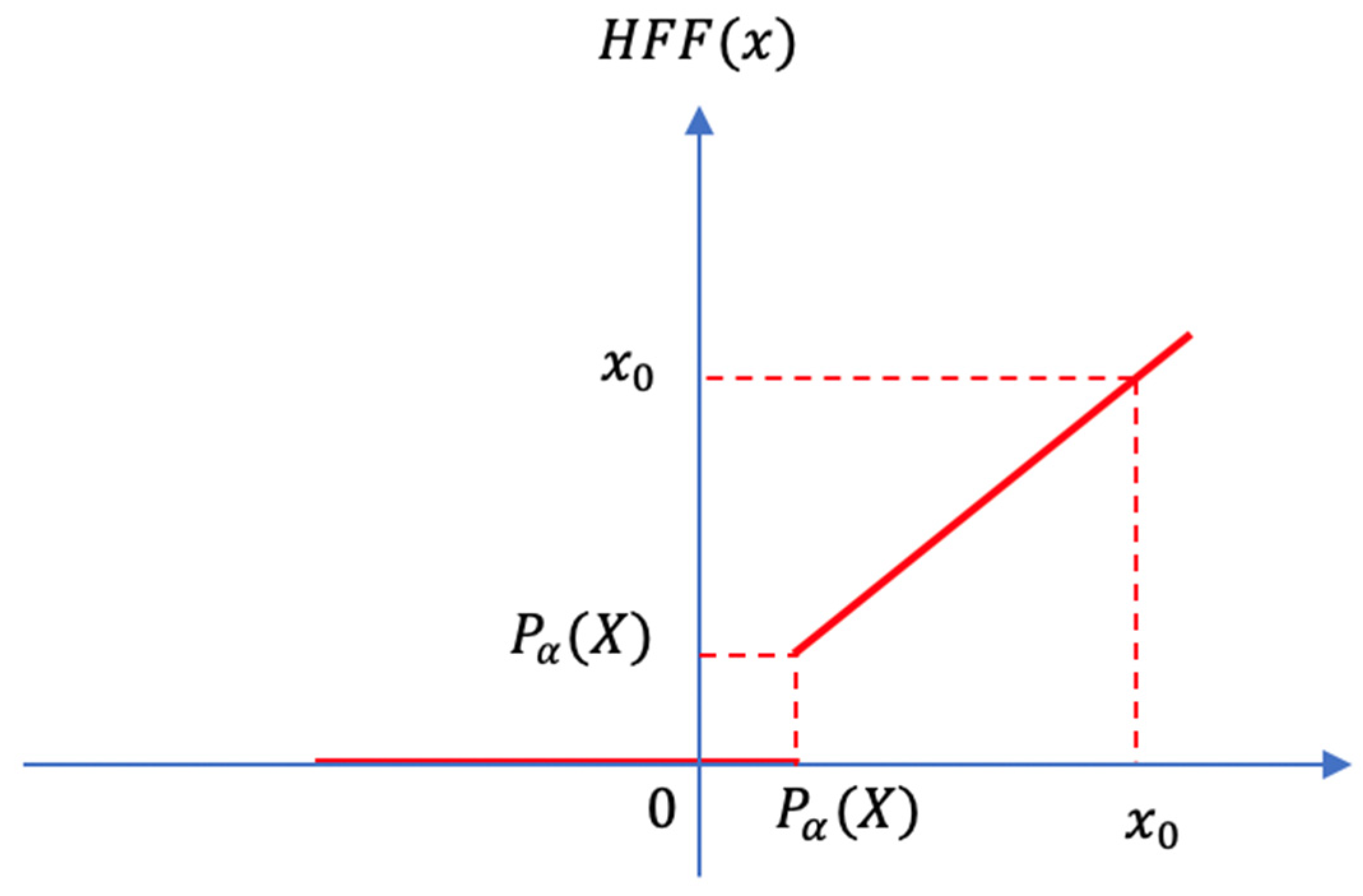
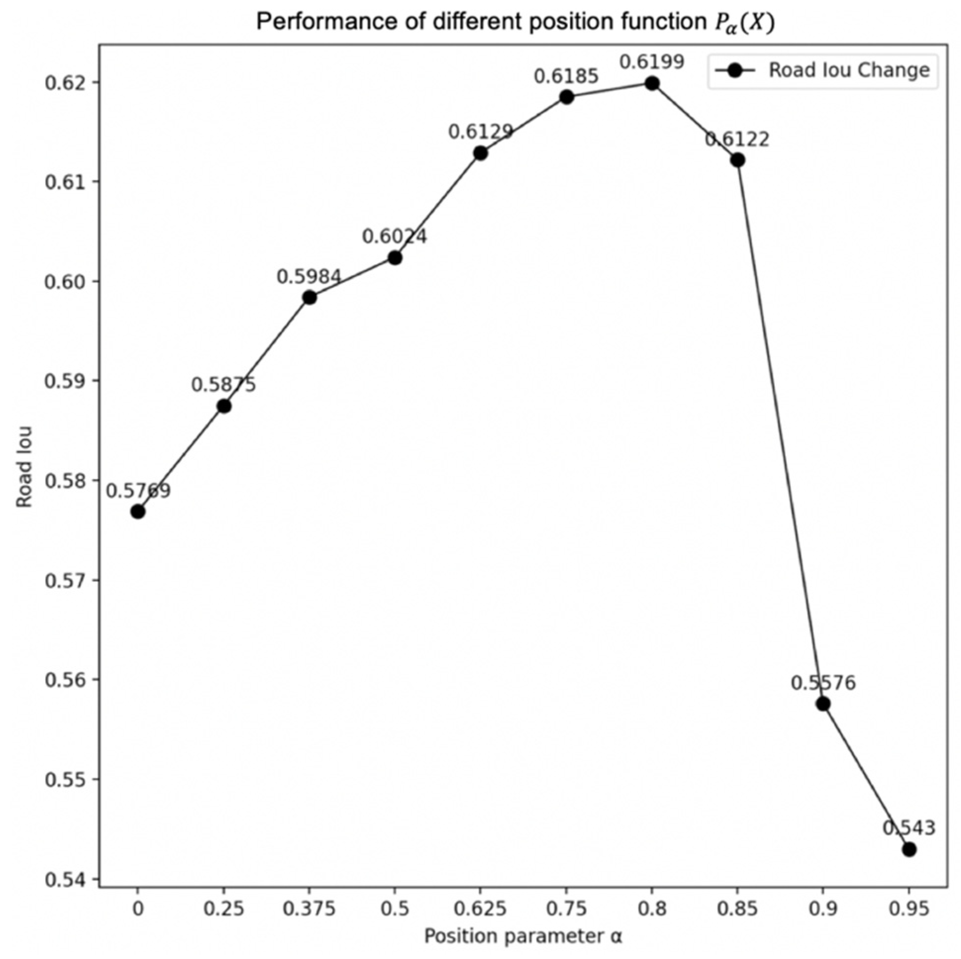
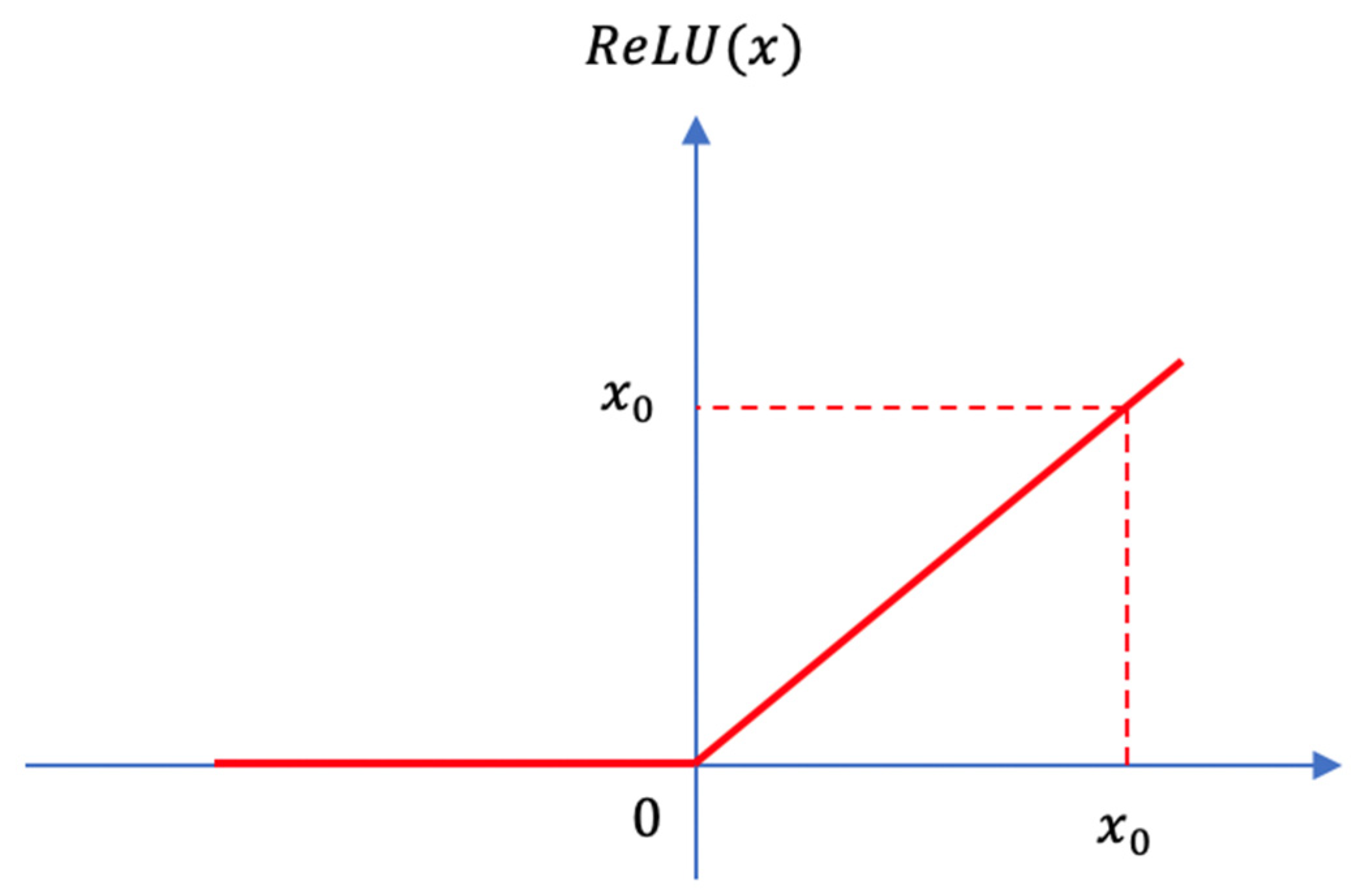
3.3. Heterogeneous Filter Function and Output Part
3.3.1. Heterogeneous Filter Function
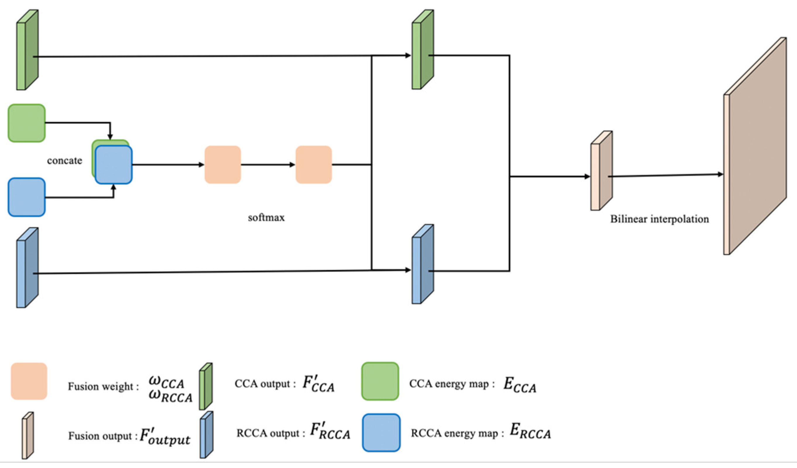
3.3.2. Output Part: SAF Module
4. Experiment
4.1. Dataset and Implement Details
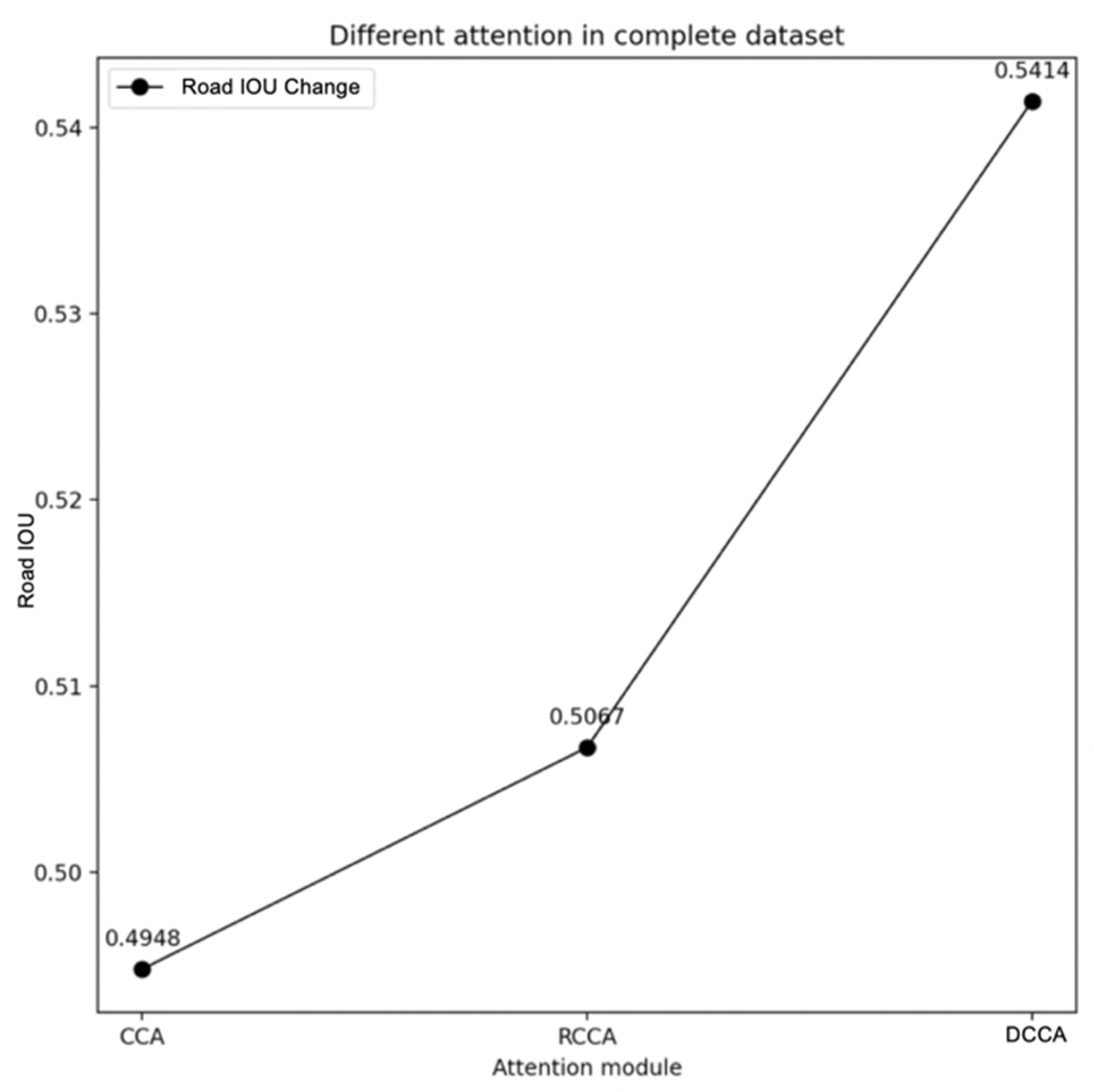
4.2. Results of Different Attention Methods
4.3. Explanation of the Result
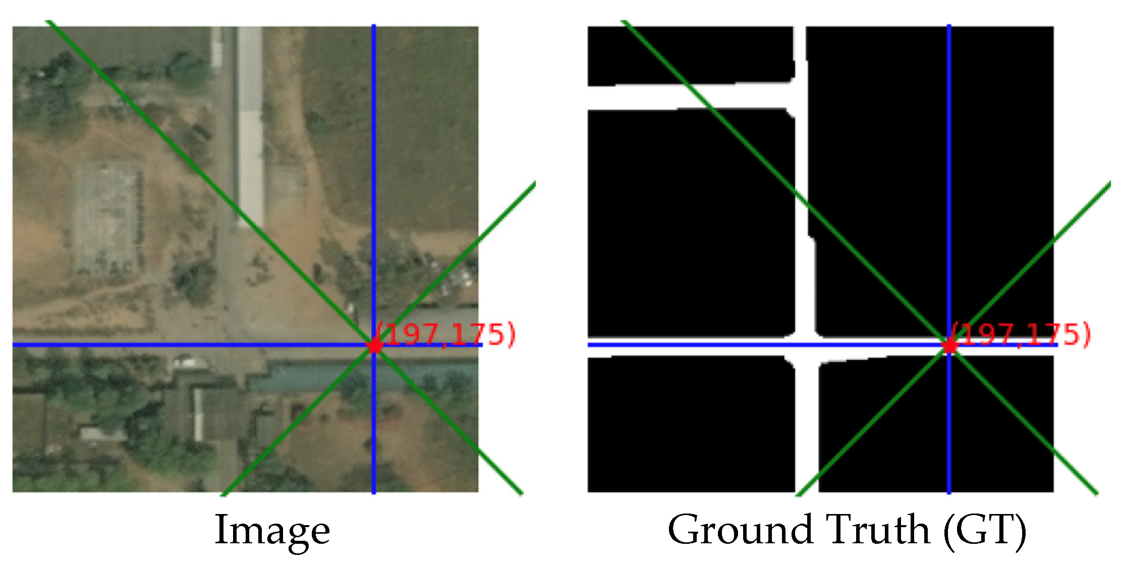
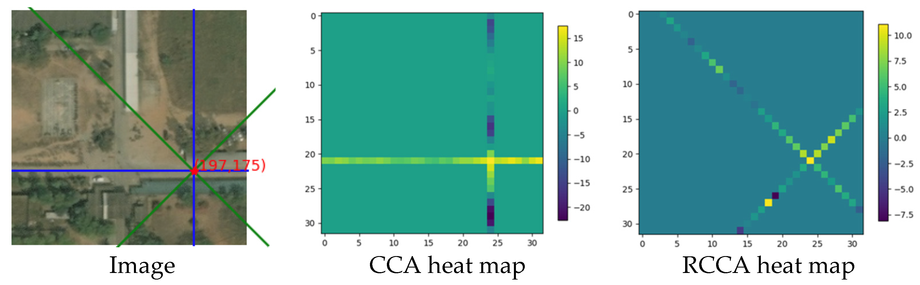
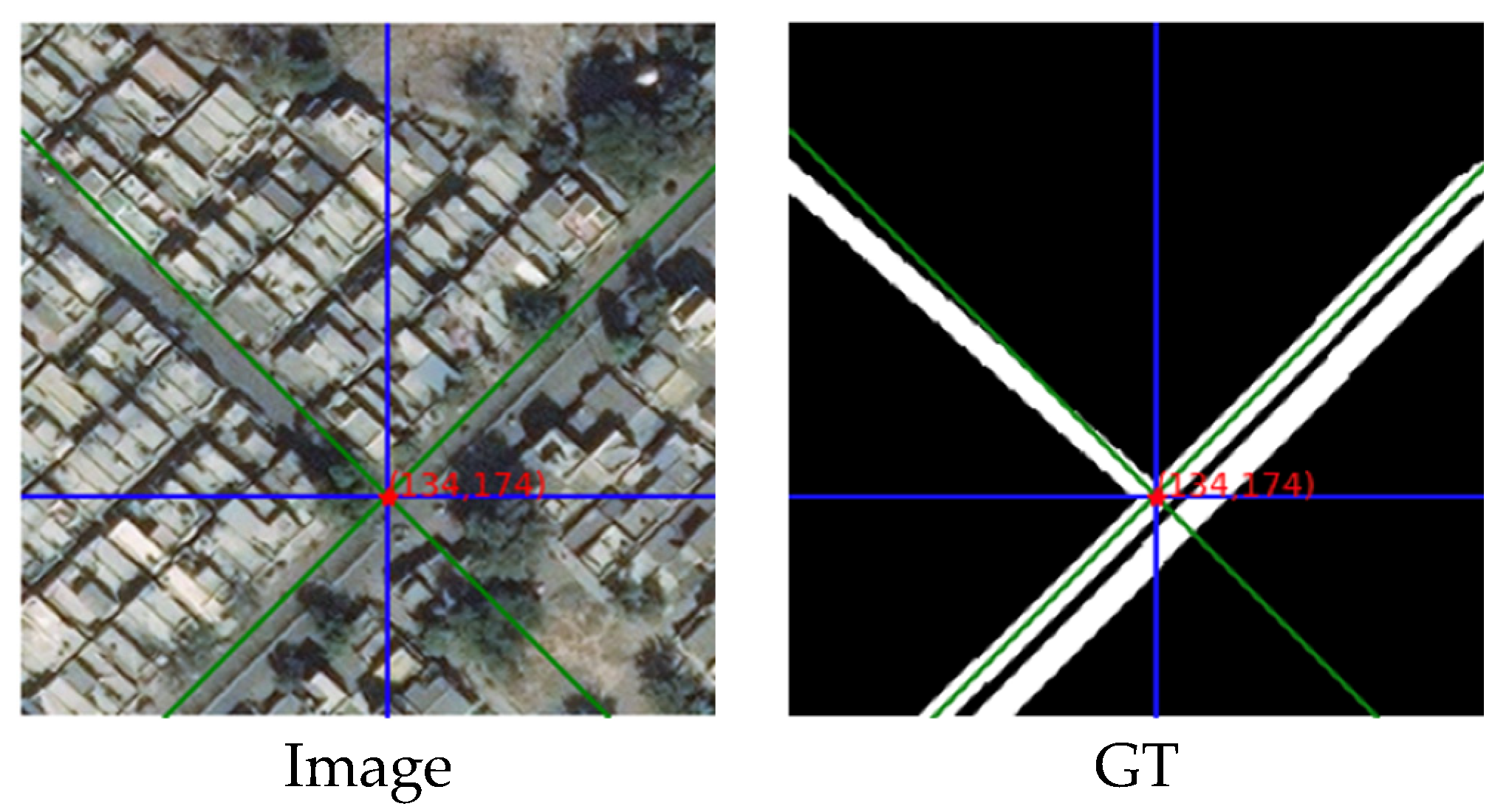
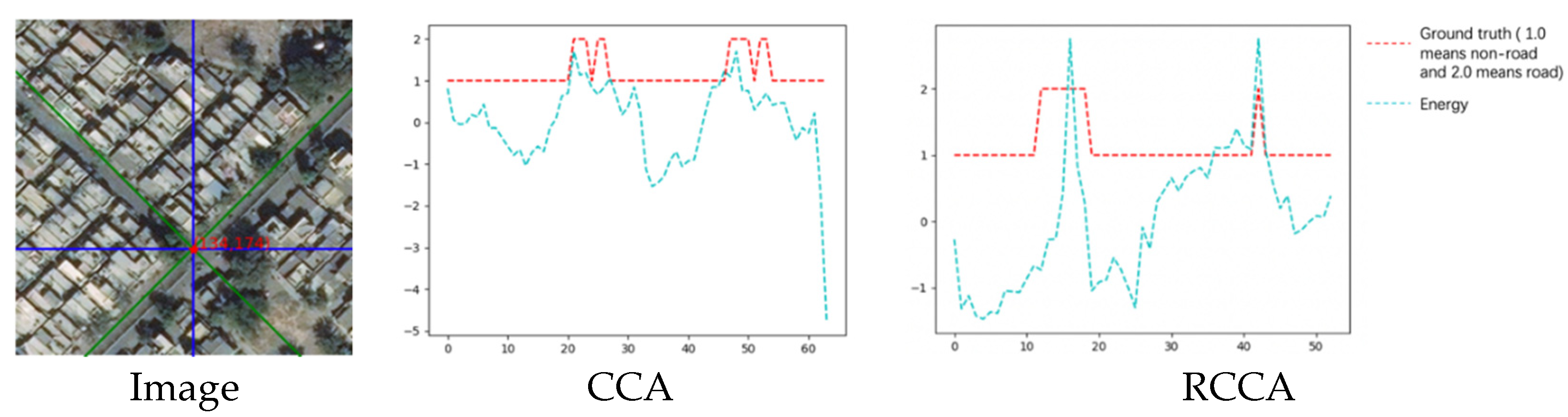
4.3.1. Example with Only Crisscross Shaped Roads
- (1)
- The energy heat map:
- (2)
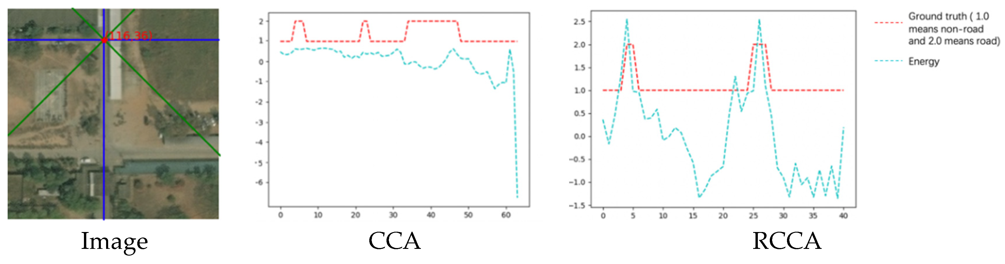
- The energy line chart:
- (3)
- The energy table:
- (4)
- The output collection:
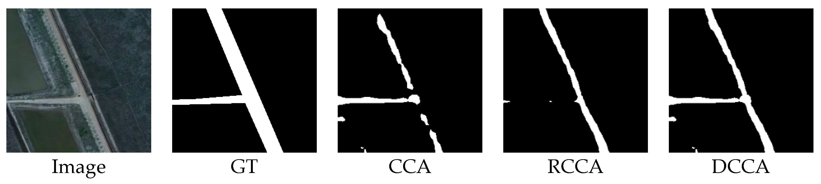
4.3.2. Example with Only Rotated Crisscross Shaped Roads
- (1)
- The energy line chart:
- (2)
- The energy table:
- (3)
- The output collection:
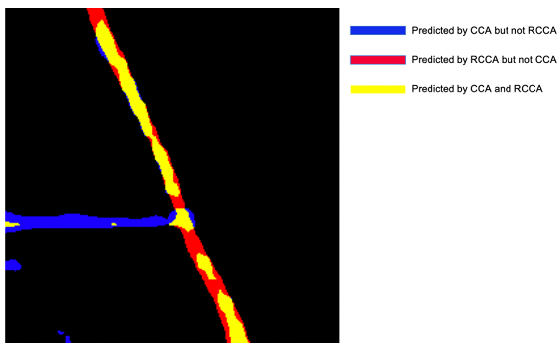
4.3.3. Example with Both Crisscross Shaped Roads and Rotated Crisscross Shaped Roads
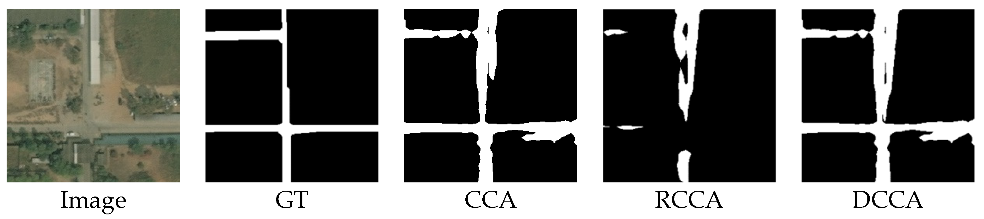
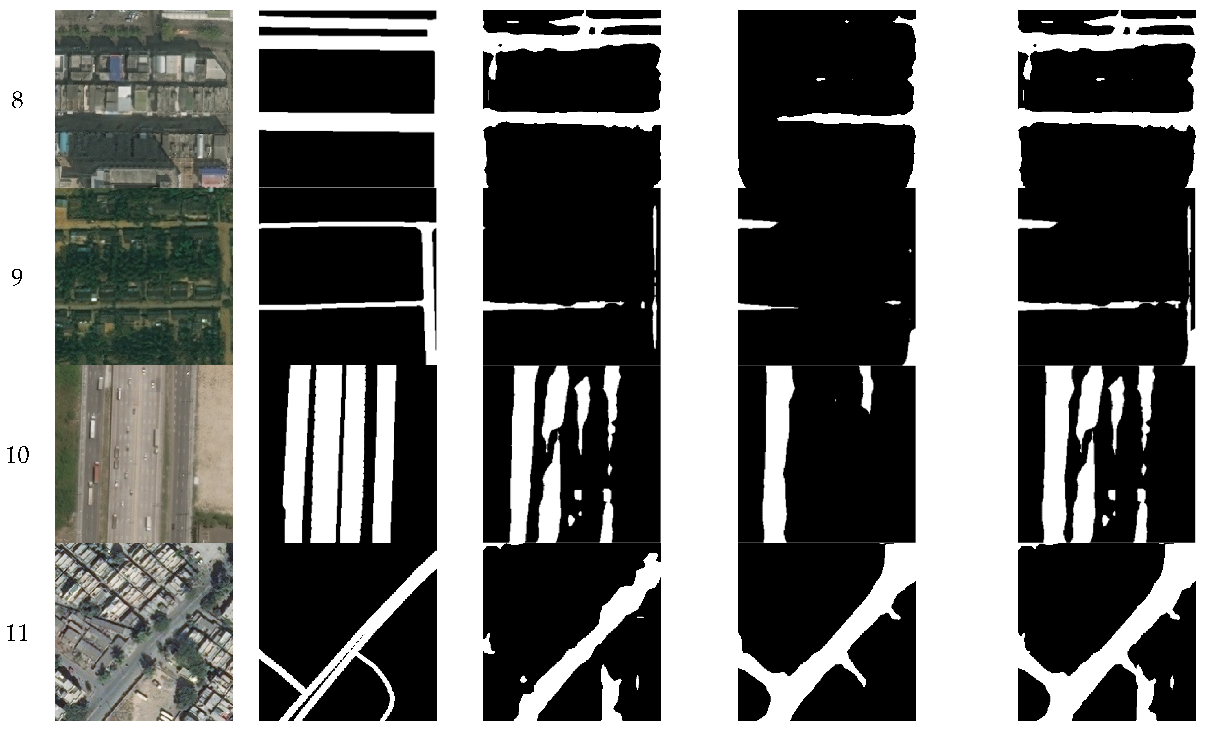
4.4. Some Typical Examples
5. Conclusions
Author Contributions
Funding
Informed Consent Statement
Conflicts of Interest
References
- Geng, K.; Sun, X.; Yan, Z.; Diao, W.; Gao, X. Topological Space Knowledge Distillation for Compact Road Extraction in Optical Remote Sensing Images. Remote Sens. 2020, 12, 3175. [Google Scholar] [CrossRef]
- Wang, X.; Girshick, R.; Gupta, A.; He, K. Non-local neural networks. In Proceedings of the IEEE Conference on Computer Vision and Pattern Recognition, Salt Lake City, UT, USA, 18–23 June 2018; pp. 7794–7803. [Google Scholar]
- He, H.; Wang, S.; Yang, D.; Wang, S.; Liu, X. An road extraction method for remote sensing image based on Encoder-Decoder network. Acta Geod. Cartogr. Sin. 2019, 48, 330. [Google Scholar]
- Long, J.; Shelhamer, E.; Darrell, T. Fully convolutional networks for semantic segmentation. In Proceedings of the IEEE Conference on Computer Vision and Pattern Recognition, Boston, MA, USA, 7–12 June 2015; pp. 3431–3440. [Google Scholar]
- Luo, W.; Li, Y.; Urtasun, R.; Zemel, R. Understanding the effective receptive field in deep convolutional neural networks. arXiv 2016, arXiv:1701.04128. [Google Scholar]
- Liu, W.; Rabinovich, A.; Berg, A.C. Parsenet: Looking wider to see better. arXiv 2015, arXiv:1506.04579. [Google Scholar]
- Yu, F.; Koltun, V. Multi-scale context aggregation by dilated convolutions. arXiv 2015, arXiv:1511.07122. [Google Scholar]
- Huang, Z.; Wang, X.; Huang, L.; Huang, C.; Wei, Y.; Liu, W. Ccnet: Criss-cross attention for semantic segmentation. In Proceedings of the IEEE/CVF International Conference on Computer Vision, Seoul, Korea, 27 October–2 November 2019; pp. 603–612. [Google Scholar]
- Woo, S.; Park, J.; Lee, J.Y.; Kweon, I.S. Cbam: Convolutional block attention module. In Proceedings of the European conference on computer vision (ECCV), Munich, Germany, 8–14 September 2018; pp. 3–19. [Google Scholar]
- LeCun, Y.; Bottou, L.; Bengio, Y.; Haffner, P. Gradient-based learning applied to document recognition. Proc. IEEE 1998, 86, 2278–2324. [Google Scholar] [CrossRef] [Green Version]
- Krizhevsky, A.; Sutskever, I.; Hinton, G.E. Imagenet classification with deep convolutional neural networks. Adv. Neural Inf. Process. Syst. 2012, 25, 1097–1105. [Google Scholar] [CrossRef]
- Ronneberger, O.; Fischer, P.; Brox, T. U-Net: Convolutional Networks for Biomedical Image Segmentation. In Medical Image Computing and Computer-Assisted Intervention—MICCAI 2015; Springer: Cham, Switzerland, 2015. [Google Scholar]
- Badrinarayanan, V.; Kendall, A.; Cipolla, R. Segnet: A deep convolutional encoder-decoder architecture for image segmentation. IEEE Trans. Pattern Anal. Mach. Intell. 2017, 39, 2481–2495. [Google Scholar] [CrossRef]
- Chen, L.C.; Papandreou, G.; Kokkinos, I.; Murphy, K.; Yuille, A.L. Deeplab: Semantic image segmentation with deep convolutional nets, atrous convolution, and fully connected crfs. IEEE Trans. Pattern Anal. Mach. Intell. 2017, 40, 834–848. [Google Scholar] [CrossRef]
- Chen, L.C.; Papandreou, G.; Schroff, F.; Adam, H. Rethinking atrous convolution for semantic image segmentation. arXiv 2017, arXiv:1706.05587. [Google Scholar]
- Chen, L.C.; Zhu, Y.; Papandreou, G.; Schroff, F.; Adam, H. Encoder-decoder with atrous separable convolution for semantic image segmentation. In Proceedings of the European Conference on Computer Vision (ECCV), Munich, Germany, 8–14 September 2018; pp. 801–818. [Google Scholar]
- Zhao, H.; Shi, J.; Qi, X.; Wang, X.; Jia, J. Pyramid scene parsing network. In Proceedings of the IEEE Conference on Computer Vision and Pattern Recognition, Honolulu, HI, USA, 21–26 July 2017; pp. 2881–2890. [Google Scholar]
- Zhao, H.; Zhang, Y.; Liu, S.; Shi, J.; Loy, C.C.; Lin, D.; Jia, J. Psanet: Point-wise spatial attention network for scene parsing. In Proceedings of the European Conference on Computer Vision (ECCV), Munich, Germany, 8–14 September 2018; pp. 267–283. [Google Scholar]
- Mnih, V.; Heess, N.; Graves, A. Recurrent models of visual attention. arXiv 2014, arXiv:1406.6247. [Google Scholar]
- Bahdanau, D.; Cho, K.; Bengio, Y. Neural machine translation by jointly learning to align and translate. arXiv 2014, arXiv:1409.0473. [Google Scholar]
- Vaswani, A.; Shazeer, N.; Parmar, N.; Uszkoreit, J.; Jones, L.; Gomez, A.N.; Kaiser, L.; Polosukhin, I. Attention is all you need. arXiv 2017, arXiv:1706.03762. [Google Scholar]
- Hu, J.; Shen, L.; Sun, G. Squeeze-and-excitation networks. In Proceedings of the IEEE Conference on Computer Vision and Pattern Recognition, Salt Lake City, UT, USA, 18–23 June 2018; pp. 7132–7141. [Google Scholar]
- Fu, J.; Liu, J.; Tian, H.; Li, Y.; Bao, Y.; Fang, Z.; Lu, H. Dual attention network for scene segmentation. In Proceedings of the IEEE/CVF Conference on Computer Vision and Pattern Recognition, Long Beach, CA, USA, 15–20 June 2019; pp. 3146–3154. [Google Scholar]
- Ulku, I.; Akagunduz, E. A Survey on Deep Learning-based Architectures for Semantic Segmentation on 2D images. arXiv 2019, arXiv:1912.10230. [Google Scholar]
- Cordonnier, J.B.; Loukas, A.; Jaggi, M. On the Relationship between Self-Attention and Convolutional Layers. arXiv 2019, arXiv:1911.03584. [Google Scholar]
- Huang, X.; Zhang, L. Road centreline extraction from high-resolution imagery based on multiscale structural features and support vector machines. Int. J. Remote Sens. 2009, 30, 1977–1987. [Google Scholar] [CrossRef]
- Mnih, V.; Hinton, G.E. Learning to detect roads in high-resolution aerial images. In European Conference on Computer Vision; Springer: Berlin/Heidelberg, Germany, 2010; pp. 210–223. [Google Scholar]
- Unsalan, C.; Sirmacek, B. Road network detection using probabilistic and graph theoretical methods. IEEE Trans. Geosci. Remote. Sens. 2012, 50, 4441–4453. [Google Scholar] [CrossRef]
- Cheng, G.; Wang, Y.; Gong, Y.; Zhu, F.; Pan, C. Urban road extraction via graph cuts based probability propagation. In Proceedings of the 2014 IEEE International Conference on Image Processing (ICIP), Paris, France, 27–30 October 2014; pp. 5072–5076. [Google Scholar]
- Saito, S.; Yamashita, T.; Aoki, Y. Multiple object extraction from aerial imagery with convolutional neural networks. Electron. Imaging 2016, 2016, 1–9. [Google Scholar] [CrossRef]
- Alshehhi, R.; Marpu, P.R. Hierarchical graph-based segmentation for extracting road networks from high-resolution satellite images. ISPRS J. Photogramm. Remote Sens. 2017, 126, 245–260. [Google Scholar] [CrossRef]
- Liu, B.; Wu, H.; Wang, Y.; Liu, W. Main road extraction from zy-3 grayscale imagery based on directional mathematical morphology and vgi prior knowledge in urban areas. PLoS ONE 2015, 10, e0138071. [Google Scholar] [CrossRef] [Green Version]
- Sujatha, C.; Selvathi, D. Connected component-based technique for automatic extraction of road centerline in high resolution satellite images. EURASIP J. Image Video Process. 2015, 2015, 1–16. [Google Scholar] [CrossRef] [Green Version]
- Cheng, G.; Wang, Y.; Xu, S.; Wang, H.; Xiang, S.; Pan, C. Automatic road detection and centerline extraction via cascaded end-to-end convolutional neural network. IEEE Trans. Geosci. Remote Sens. 2017, 55, 3322–3337. [Google Scholar] [CrossRef]
- Cheng, G.; Zhu, F.; Xiang, S.; Pan, C. Road centerline extraction via semisupervised segmentation and multidirection nonmaximum suppression. IEEE Geosci. Remote Sens. Lett. 2016, 13, 545–549. [Google Scholar] [CrossRef]
- Qiaoping, Z.; Couloigner, I. Automatic road change detection and GIS updating from high spatial remotely-sensed imagery. Geo-Spat. Inf. Sci. 2004, 7, 89–95. [Google Scholar] [CrossRef] [Green Version]
- Song, M.; Civco, D. Road extraction using SVM and image segmentation. Photogramm. Eng. Remote Sens. 2004, 70, 1365–1371. [Google Scholar] [CrossRef] [Green Version]
- Das, S.; Mirnalinee, T.T.; Varghese, K. Use of salient features for the design of a multistage framework to extract roads from high-resolution multispectral satellite images. IEEE Trans. Geosci. Remote Sens. 2011, 49, 3906–3931. [Google Scholar] [CrossRef]
- Alvarez, J.M.; Gevers, T.; LeCun, Y.; Lopez, A.M. Road scene segmentation from a single image. In European Conference on Computer Vision; Springer: Berlin/Heidelberg, Germany, 2012; pp. 376–389. [Google Scholar]
- Zhong, Z.; Li, J.; Cui, W.; Jiang, H. Fully convolutional networks for building and road extraction: Preliminary results. In Proceedings of the 2016 IEEE International Geoscience and Remote Sensing Symposium (IGARSS), Beijing, China, 10–15 July 2016; pp. 1591–1594. [Google Scholar]
- Zhang, Z.; Liu, Q.; Wang, Y. Road extraction by deep residual u-net. IEEE Geosci. Remote Sens. Lett. 2018, 15, 749–753. [Google Scholar] [CrossRef] [Green Version]
- Peng, B.; Li, Y.; Fan, K.; Yuan, L.; Tong, L.; He, L. New Network Based on D-Linknet and Densenet for High Resolution Satellite Imagery Road Extraction. In Proceedings of the IGARSS 2019-2019 IEEE International Geoscience and Remote Sensing Symposium, Yokohama, Japan, 28 July–2 August 2019; pp. 3939–3942. [Google Scholar]
- Demir, I.; Koperski, K.; Lindenbaum, D.; Pang, G.; Huang, J.; Basu, S.; Hughes, F.; Tuia, D.; Raskar, R. DeepGlobe 2018: A Challenge to Parse the Earth through Satellite Images. In Proceedings of the2018 IEEE/CVF Conference on Computer Vision and Pattern Recognition Workshops (CVPRW), Salt Lake City, UT, USA, 18–22 June 2018; pp. 172–181. [Google Scholar] [CrossRef] [Green Version]


| Indicators | Complete Dataset | CC Dataset | RCC Dataset |
|---|---|---|---|
| Road IOU | 0.4948 | 0.5442 | 0.4498 |
| Mean IOU | 0.7030 | 0.7327 | 0.6759 |
| Indicators | Complete Dataset | CC Dataset | RCC Dataset |
|---|---|---|---|
| Road IOU | 0.5067 | 0.5242 | 0.4909 |
| Mean IOU | 0.7117 | 0.7229 | 0.7015 |
| Indicators | Complete Dataset | CC Dataset | RCC Dataset |
|---|---|---|---|
| Road IOU | 0.5414 | 0.5722 | 0.5140 |
| Mean IOU | 0.7256 | 0.7454 | 0.7077 |
| Indicators | CCA | RCCA | DCCA |
|---|---|---|---|
| Road IOU | 0.4948 | 0.5067 | 0.5414 |
| Mean IOU | 0.7030 | 0.7117 | 0.7256 |
| Models | Road IOU | Mean IOU |
|---|---|---|
| DCCA | 0.5414 | 0.7256 |
| DCCA (with 30°) | 0.5275 | 0.7282 |
| Non-local CBAM PSPNet | 0.5411 0.5325 0.5357 | 0.7372 0.7318 0.7322 |
| Classification | CCA | RCCA |
|---|---|---|
| Road | 10.21 | 7.96 |
| Non-road | 7.95 | −0.14 |
| Classification | CCA | RCCA |
|---|---|---|
| Road | 6.97 | 5.75 |
| Non-road | 1.12 | 3.43 |
Publisher’s Note: MDPI stays neutral with regard to jurisdictional claims in published maps and institutional affiliations. |
© 2021 by the authors. Licensee MDPI, Basel, Switzerland. This article is an open access article distributed under the terms and conditions of the Creative Commons Attribution (CC BY) license (https://creativecommons.org/licenses/by/4.0/).
Share and Cite
Chen, C.; Zhao, H.; Cui, W.; He, X. Dual Crisscross Attention Module for Road Extraction from Remote Sensing Images. Sensors 2021, 21, 6873. https://doi.org/10.3390/s21206873
Chen C, Zhao H, Cui W, He X. Dual Crisscross Attention Module for Road Extraction from Remote Sensing Images. Sensors. 2021; 21(20):6873. https://doi.org/10.3390/s21206873
Chicago/Turabian StyleChen, Chuan, Huilin Zhao, Wei Cui, and Xin He. 2021. "Dual Crisscross Attention Module for Road Extraction from Remote Sensing Images" Sensors 21, no. 20: 6873. https://doi.org/10.3390/s21206873
APA StyleChen, C., Zhao, H., Cui, W., & He, X. (2021). Dual Crisscross Attention Module for Road Extraction from Remote Sensing Images. Sensors, 21(20), 6873. https://doi.org/10.3390/s21206873