An Accurate Linear Method for 3D Line Reconstruction for Binocular or Multiple View Stereo Vision

Abstract
1. Introduction
2. Direction-then-Point Method
2.1. Stereo-Vision Scenario
2.2. Plane Representation by a Single Camera
2.3. Plane Intersection
3. Point-then-Direction Method
3.1. Stereo Vision Scenario for PtD
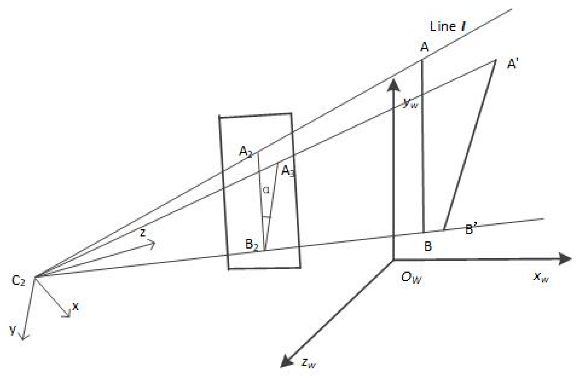
3.2. Image-Space Angle Residual
3.2.1. Definition of the Problem
3.2.2. Linear Method
3.2.3. Efficiency Analysis
- Solve the 3D coordinate of the corresponding image points with a time complexity of ;
- Solve the line parameters projected onto the image plane with a time complexity of ;
- Solve the coefficient matrix with a time complexity of ;
- Find the final result in fixed time.
4. Experiments
4.1. Simulation
4.1.1. Simulation Environment
4.1.2. Simulation Description
- The corresponding image points used in the PtD method were obtained by adding the same error to the projection of the endpoint A in the image, which ensured that PtD method was also solved under the same error conditions.
- The TPS, DtP, and PtD methods were used for each simulation. We used the angle between the result and the ground truth and the distance from the two endpoints to the result line to evaluate the accuracy. All simulations were calculated 1000 times, and the root mean square (RMS) of the angular error and the average of distance were obtained. The units of angular error were degrees, and the units of distance error were meters.
- Angle between optical axes of binocular cameras.
- 3D line’s attitude.
- Line segments extraction error in image.
- Errors of all camera external parameters.
- All camera external parameters and extraction errors.
- Number of cameras.
- Running time.
4.1.3. Simulation Results
4.1.4. Simulation Conclusion
- Under the same error of the external camera parameters and the 2D line, the PtD method has the best directional accuracy, and the TPS method has the best positional accuracy.
- When the intersection condition was normal, the 3D line’s direction accuracy of the three methods, from most to least accurate, was PtD, DtP, then TPS, and the 3D line’s position accuracy of the three methods, from most to least accurate, was TPS, PtD, and DtP. Therefore, if the direction accuracy is more important, the PtD method should be used, and if positional accuracy is more important, the TPS method should be used—provided that there are two pairs of corresponding image points.
- When the intersection condition was bad and the target was relative long, TPS achieved the best accuracy, both in the direction and position of the 3D line. However, it needs two pairs of corresponding image points, which is sometimes hard to satisfy. PtD achieved better accuracy than DtP both in the direction and position of the 3D line, so PtD can be used if there is only one pair of corresponding image points.
4.2. Physical Experiment
4.2.1. Physical Experiment 1
Physical Environment
Experimental Procedure
- The world coordinate system was established by the total station. The total station was used to obtain the coordinates of the calibration control points. The coordinate system direction was vertically upwards (Y) and horizontal (XZ), and the system constituted a right-hand coordinate system.
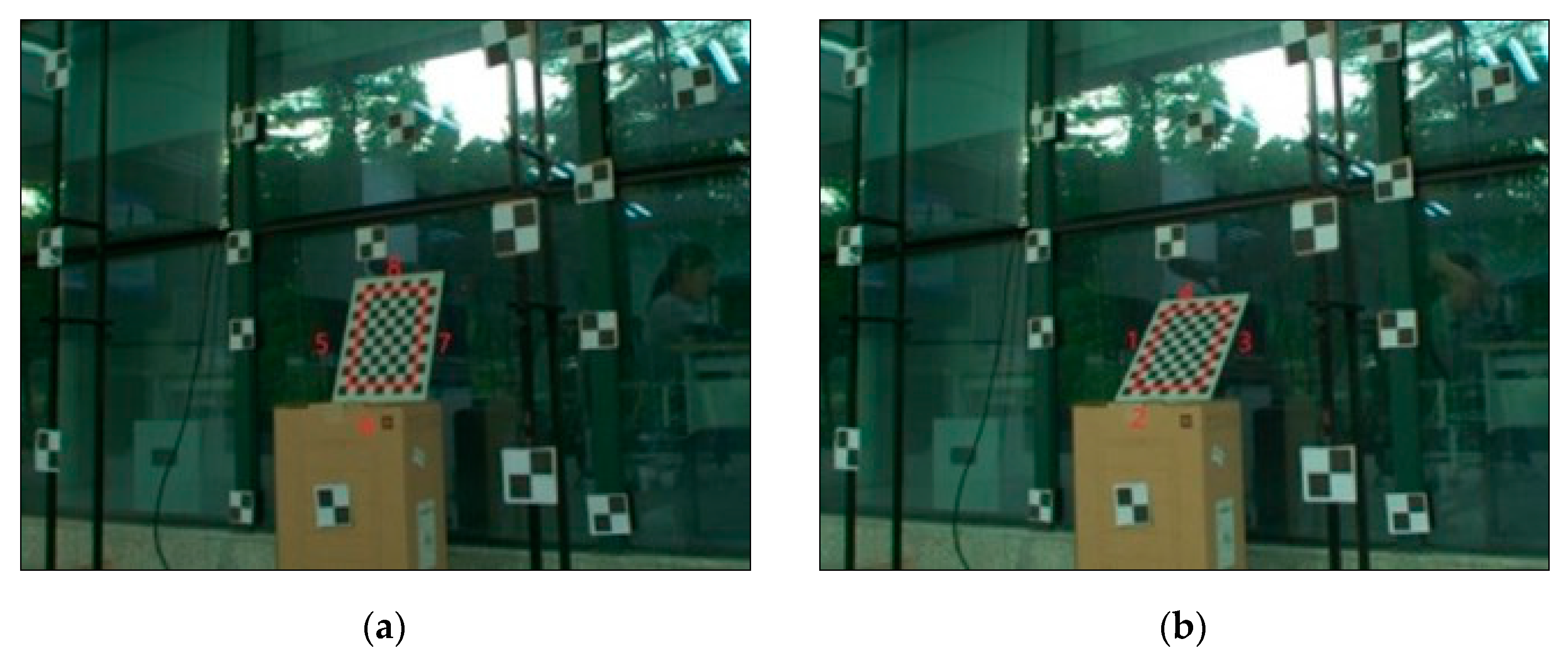
- The stereo cameras were used to take photos synchronously. The checkerboard was placed at two angles to verify the accuracy of the methods in two conditions. One was where the 3D lines were parallel to the imaging plane, and the other was not. The calibration control points were extracted from the image, and the 3D coordinates were used to calibrate all of the cameras in a unified world coordinate system. All parameters of the camera were calibrated, including the main point, equivalent focal length, lens distortion, and external parameters of the camera.
- The 2D lines and the corresponding image points were extracted from the two images by extracted the two endpoints of the 2D lines. The corresponding image points were one of the endpoints of the 2D lines.
- After the correction of lens distortion, DtP, PtD, and TPS were used separately to obtain the 3D line I.
4.2.2. Physical Experiment 2
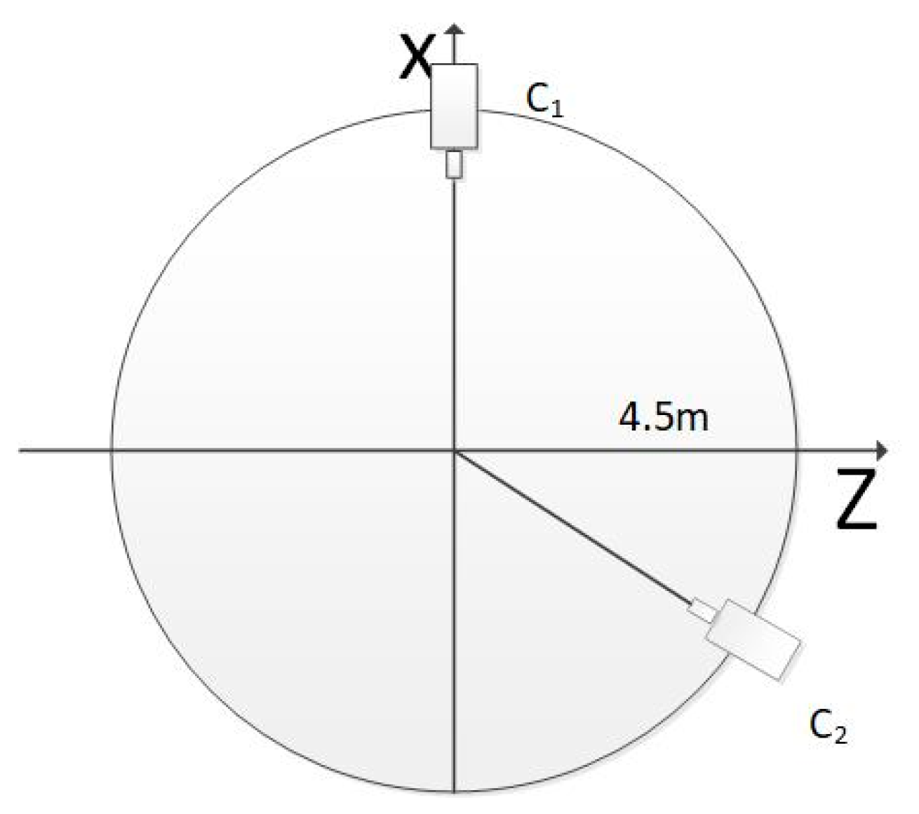
Physical Environment
Experimental Procedure
- The total station was used to obtain the coordinates of the calibration control points in the world coordinate system. The total station coordinate system was used as the world coordinate system. The coordinate system direction was vertically upwards (Y) and horizontal (XZ) and the system constituted a right-hand coordinate system.
- The same camera was used to take photographs from nine different locations. The calibration control points were extracted from the image, and the three-dimensional coordinates were used to calibrate all of the cameras in a unified world coordinate system.
- The 2D line was extracted from the image. The corresponding image point was the top point of the target.
- DtP and PtD were used separately to obtain the results. For hard-to-find pairs of corresponding image points on the target, TPS was not used.
5. Conclusions
Author Contributions
Funding
Informed Consent Statement
Data Availability Statement
Conflicts of Interest
References
- Liu, L.; Zhao, Z. A new approach for measurement of pitch, roll and yaw angles based on a circular feature. Trans. Inst. Meas. Control 2013, 35, 384–397. [Google Scholar] [CrossRef]
- Hao, W.; Zhang, X.; Huang, Y.; Yang, F.; Guo, B. Determining relative position and attitude of a close non-cooperative target based on the SIFT algorithm. J. Beijing Inst. Technol. 2014, 3, 110–114. [Google Scholar]
- Yin, F.; Chou, W.; Wu, Y.; Yang, G.; Xu, S. Sparse unorganized point cloud based relative pose estimation for uncooperative space target. Sensors 2018, 18, 1009. [Google Scholar] [CrossRef] [PubMed]
- He, Y.; Liang, B.; He, J.; Li, S. Non-cooperative spacecraft pose tracking based on point cloud feature. Acta Astronaut. 2017, 139, 213–221. [Google Scholar] [CrossRef]
- Peng, J.; Xu, W.; Yuan, H. An efficient pose measurement method of a space non-cooperative target based on stereo vision. IEEE Access 2017, 5, 22344–22362. [Google Scholar] [CrossRef]
- Peng, J.; Xu, W.; Liang, B.; Wu, A.G. Pose measurement and motion estimation of space non-cooperative targets based on laser radar and stereo-vision fusion. IEEE Sens. J. 2018, 19, 3008–3019. [Google Scholar] [CrossRef]
- Yu, F.; He, Z.; Qiao, B.; Yu, X. Stereo-vision-based relative pose estimation for the rendezvous and docking of noncooperative satellites. Math. Probl. Eng. 2014, 2014, 1–12. [Google Scholar] [CrossRef]
- Du, X.; Liang, B.; Xu, W.; Qiu, Y. Pose measurement of large non-cooperative satellite based on collaborative cameras. Acta Astronaut. 2011, 68, 2047–2065. [Google Scholar] [CrossRef]
- Miao, X.; Zhu, F.; Hao, Y. Pose estimation of non-cooperative spacecraft based on collaboration of space-ground and rectangle feature. In Proceedings of the International Symposium on Photoelectronic Detection and Imaging 2011: Space Exploration Technologies and Applications, Beijing, China, 24–26 May 2011; Volume 8196. [Google Scholar]
- Kannan, S.K.; Johnson, E.N.; Watanabe, Y.; Sattigeri, R. Vision-based tracking of uncooperative targets. Int. J. Aerosp. Eng. 2011, 2011, 1–17. [Google Scholar] [CrossRef]
- Baillard, C.; Schmid, C.; Zisserman, A.; Fitzgibbon, A. Automatic line matching and 3D reconstruction of buildings from multiple views. In Proceedings of the ISPRS Conference on Automatic Extraction of GIS Objects from Digital Imagery, Munich Germany, 8–10 September 1999; Volume 32, pp. 69–80. [Google Scholar]
- Yu, Q.; Sun, X.; Chen, G. A new method of measure the pitching and yaw of the axes symmetry object through the optical image. J. Natl. Univ. Def. Technol. 2000, 22, 15–19. [Google Scholar]
- Hartley, R.; Zisserman, A. Multiple View Geometry in Computer Vision; Cambridge University Press: Cambridge, UK, 2003. [Google Scholar]
- Ok, A.Ö.; Wegner, J.D.; Heipke, C.; Rottensteiner, F.; Soergel, U.; Toprak, V. Accurate reconstruction of near-epipolar line segments from stereo aerial images. Photogramm. Fernerkund. Geoinf. 2012, 2012, 345–358. [Google Scholar] [CrossRef]
- Ding, S. Research on Axis Extraction Methods for Target’s Attitude Measurement; National University of Defense Technology: Changsha, China, 2013. [Google Scholar]
- Zhang, Y.; Wang ZH, Q.; Qiao, Y.F. Attitude measurement method research for missile launch. Chin. Opt. 2015, 8, 997–1003. [Google Scholar] [CrossRef]
- Luo, K.; Fan, L.; Gao, Y.; Zhang, H.; Li, Q.A.; Zhu, Y. Measuring technology on elevation angle and yawing angle of space target based on optical measurement method. J. Changchun Univ. Sci.Technol. 2007, 30, 12–14. [Google Scholar]
- Wang, C. Study on Methods to Improve the Attitude Measurement Precision of the Rotary Object; University of Chinese Academy of Sciences (Institute of Optics and Electronics): Chengdu, China, 2013. [Google Scholar]
- Chen, M.; Tang, Y.; Zou, X.; Huang, K.; Huang, Z.; Zhou, H.; Wang, C.; Lian, G. Three-dimensional perception of orchard banana central stock enhanced by adaptive multi-vision technology. Comput. Electron. Agric. 2020, 174, 105508. [Google Scholar] [CrossRef]
- Tang, Y.C.; Wang, C.; Luo, L.; Zou, X. Recognition and localization methods for vision-based fruit picking robots: A review. Front. Plant Sci. 2020, 11, 510. [Google Scholar] [CrossRef] [PubMed]
- Li, Y.; Bo, Y.; Zhao, G. Survey of measurement of position and pose for space non-cooperative target. In Proceedings of the IEEE 34th Chinese Control Conference (CCC), Hanghzou, China, 28–30 July 2015; pp. 5101–5106. [Google Scholar]
- Pesce, V.; Lavagna, M.; Bevilacqua, R. Stereovision-based pose and inertia estimation of unknown and uncooperative space objects. Adv. Space Res. 2017, 59, 236–251. [Google Scholar] [CrossRef]
- Opromolla, R.; Fasano, G.; Rufino, G.; Grassi, M. A model-based 3D template matching technique for pose acquisition of an uncooperative space object. Sensors 2015, 15, 6360–6382. [Google Scholar] [CrossRef]
- Yuan, Y. Research on Networked Videometrics for the Shape and Deformation of Large-Scale Structure; National University of Defense Technology: Changsha, China, 2013. [Google Scholar]
- Golub, G.H. Singular value decomposition and least squares solutions. Numerische Mathematik 1970, 14, 403–420. [Google Scholar] [CrossRef]
- Madsen, K.; Nielsen, H.B.; Tingleff, O. Methods for Non-Linear Least Squares Problems, 2nd ed.; Informatics and Mathematical Modelling, Technical University of Denmark: Lyngby, Denmark, 2004. [Google Scholar]


| Difference | DTP | PtD | TPS |
|---|---|---|---|
| Pairs of corresponding image points | 0 | 1 | 2 |
| Can be reconstructed while the line is coplanar with the baseline (no point on the baseline) | × | × | ✓ |
| Can be reconstructed while the line is coplanar with the baseline (one point on the baseline) | × | × | × |
| Use of the camera’s optical center | × | ✓ | ✓ |
| Use of the information of the 2D line | ✓ | ✓ | × |
| Method | Case 1 | Case 2 | Case 3 | Case 4 | Case 5 | Case 6 | ||
|---|---|---|---|---|---|---|---|---|
| Perpendicular | Not Perpendicular | 90° | 120° | |||||
| (A)DtP | S | F | S→T | S→T | T | S | S | S |
| PtD | F | F | F→S | F→S | S | F | F | F |
| TPS | T | S | T→F | T→F | F | T | T | T |
| DtP(D) | T | S | T | T | T | T | T | T |
| PtD | S | S | S | S | S | S | S | S |
| TPS | F | F | F | F | F | F | F | F |
| Line No. | Measured Distance | Ideal Distance |
|---|---|---|
| 1 | 300.0 | 300.0 |
| 2 | 210.1 | 210.0 |
| 3 | 300.2 | 300.0 |
| 4 | 210.0 | 210.0 |
| 5 | 300.1 | 300.0 |
| 6 | 210.1 | 210.0 |
| 7 | 300.0 | 300.0 |
| 8 | 210.0 | 210.0 |
| Point No. | X | Y | Z |
|---|---|---|---|
| 1 | −0.2 | −0.7 | −0.0 |
| 2 | −0.5 | −0.5 | −0.1 |
| 3 | −0.2 | −0.6 | −0.0 |
| 4 | 0.4 | −0.5 | 0.8 |
| 5 | −0.4 | −0.2 | 0.6 |
| 6 | −0.0 | −0.0 | 0.1 |
| 7 | −0.5 | −0.6 | 0.2 |
| 8 | −0.1 | −0.5 | 0.7 |
| No. | DtP | PtD | TPS | DtP | PtD | TPS |
|---|---|---|---|---|---|---|
| 1 | 0.10 | 0.10 | 0.09 | 2.4 | 1.2 | 1.4 |
| 3 | 0.10 | 0.11 | 0.12 | 1.6 | 1.5 | 1.4 |
| 5 | 0.12 | 0.12 | 0.12 | 0.9 | 0.8 | 0.7 |
| 7 | 0.06 | 0.07 | 0.08 | 1.6 | 1.5 | 1.6 |
| sum | 0.38 | 0.4 | 0.41 | 6.5 | 5 | 5.1 |
| No. | DtP | PtD | TPS | DtP | PtD | TPS |
|---|---|---|---|---|---|---|
| 2 | 0.58 | 0.28 | 0.03 | 7.7 | 2.0 | 1.1 |
| 4 | 0.78 | 0.50 | 0.23 | 6.8 | 2.0 | 1.6 |
| 6 | 0.07 | 0.07 | 0.16 | 2.9 | 0.4 | 0.7 |
| 8 | 1.07 | 1.08 | 0.08 | 4.1 | 4.3 | 1.5 |
| sum | 2.5 | 1.93 | 0.5 | 21.5 | 8.7 | 4.9 |
| Camera No. | DtP | PtD |
|---|---|---|
| 2 | (−0.012, 1, −0.014) | (−0.012, 1, −0.014) |
| 6 | (−0.020, 1, −0.022) | (−0.016, 1, −0.019) |
| 9 | (−0.017, 1, −0.012) | (−0.018, 1, −0.014) |
Publisher’s Note: MDPI stays neutral with regard to jurisdictional claims in published maps and institutional affiliations. |
© 2021 by the authors. Licensee MDPI, Basel, Switzerland. This article is an open access article distributed under the terms and conditions of the Creative Commons Attribution (CC BY) license (http://creativecommons.org/licenses/by/4.0/).
Share and Cite
Zhong, L.; Qin, J.; Yang, X.; Zhang, X.; Shang, Y.; Zhang, H.; Yu, Q. An Accurate Linear Method for 3D Line Reconstruction for Binocular or Multiple View Stereo Vision. Sensors 2021, 21, 658. https://doi.org/10.3390/s21020658
Zhong L, Qin J, Yang X, Zhang X, Shang Y, Zhang H, Yu Q. An Accurate Linear Method for 3D Line Reconstruction for Binocular or Multiple View Stereo Vision. Sensors. 2021; 21(2):658. https://doi.org/10.3390/s21020658
Chicago/Turabian StyleZhong, Lijun, Junyou Qin, Xia Yang, Xiaohu Zhang, Yang Shang, Hongliang Zhang, and Qifeng Yu. 2021. "An Accurate Linear Method for 3D Line Reconstruction for Binocular or Multiple View Stereo Vision" Sensors 21, no. 2: 658. https://doi.org/10.3390/s21020658
APA StyleZhong, L., Qin, J., Yang, X., Zhang, X., Shang, Y., Zhang, H., & Yu, Q. (2021). An Accurate Linear Method for 3D Line Reconstruction for Binocular or Multiple View Stereo Vision. Sensors, 21(2), 658. https://doi.org/10.3390/s21020658