Evaluation Model of Autonomous Vehicles’ Speed Suitability Based on Overtaking Frequency

Abstract
1. Introduction
- We evaluate the discrepancy of driving states between autonomous vehicles and other vehicles in the traffic flow; to this end, the overtaking frequency (OTF) is proposed.
- Based on OTF and vehicle operating parameters, we propose a hierarchical algorithm that integrates horizontal and vertical safety assessments to inherit the advantages of both multi-lane and single-lane information.
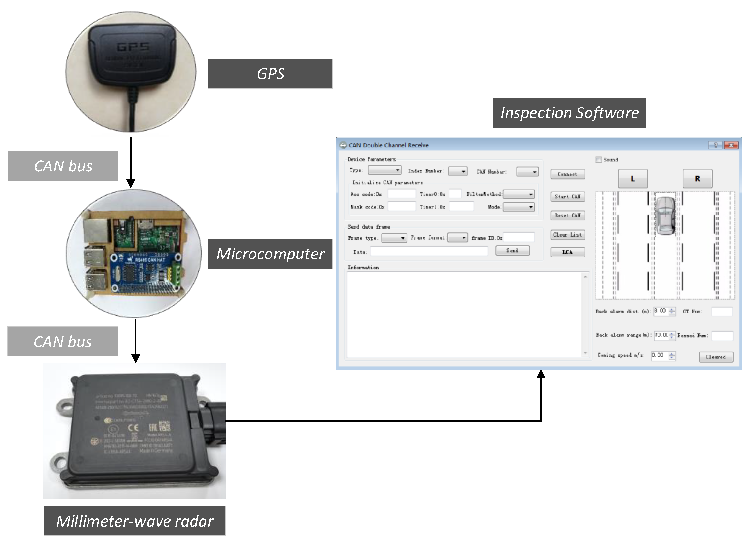
- By incorporating GPS into the Controller Area Network (CAN) bus of a millimeter-wave radar, software for detecting vehicles that are overtaking by/overtaken by on both sides of an autonomous vehicle is developed, which allows the recording of OTF.
2. Methods
2.1. OTF
2.1.1. Establishment of the OTF Factor
2.1.2. Acquisition of OTF
- Lateral vehicle recognition algorithm
- 2.
- Lateral vehicle overtaking recognition
- 3.
- Vehicle recognition algorithm for the host vehicle overtaking vehicles on the left and right sides
2.2. Speed Adaptation Evaluation Model for Different Situations
2.2.1. Case 1: No Traffic in Front of the Host Vehicle
- OTF
- 2.
- OTF or OTF
2.2.2. Case 2: Current Lane with Vehicles in Front
- OTF
- 2.
- OTF or OTF
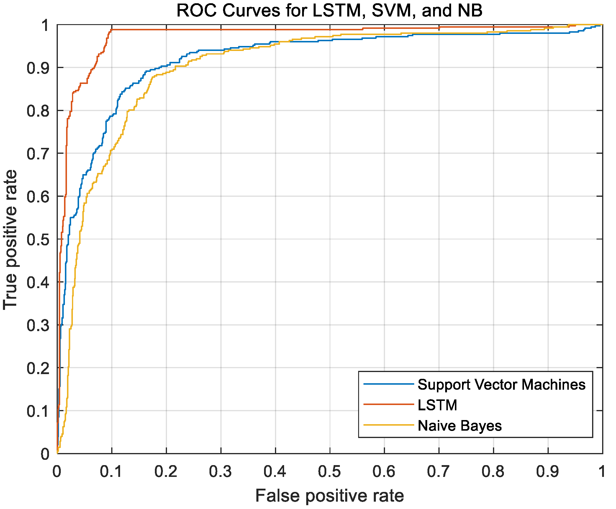
2.3. LSTM
3. Experiment
3.1. Experimental Site
3.2. Experimental Equipment
3.3. Data Collection
4. Discussion
4.1. Results of OTF
4.2. Results of the Model
4.2.1. Case 1: No Traffic in Front of the Vehicle
4.2.2. Case 2: Current Lane with Car in Front
5. Conclusions
Author Contributions
Funding
Institutional Review Board Statement
Informed Consent Statement
Data Availability Statement
Conflicts of Interest
References
- Paden, B.; Cap, M.; Yong, S.Z.; Yershov, D.; Frazzoli, E. A Survey of Motion Planning and Control Techniques for Self-Driving Urban Vehicles. IEEE Trans. Intell. Veh. 2016, 1, 33–55. [Google Scholar] [CrossRef]
- Shin, J.; Lee, I. Reliability Analysis and Reliability-Based Design Optimization of Roadway Horizontal Curves Using a First-Order Reliability Method. Eng. Optim. 2014, 47, 622–641. [Google Scholar] [CrossRef]
- Kim, S.-J.; Yoo, C.-H.; Kim, H.-K. Vulnerability Assessment for the Hazards of Crosswinds When Vehicles Cross a Bridge Deck. J. Wind. Eng. Ind. Aerodyn. 2016, 156, 62–71. [Google Scholar] [CrossRef]
- Yin, Y.; Wen, H.; Sun, L.; Hou, W. Study on the Influence of Road Geometry on Vehicle Lateral Instability. J. Adv. Transp. 2020, 2020, 1–15. [Google Scholar] [CrossRef]
- Bylykbashi, K.; Qafzezi, E.; Ampririt, P.; Ikeda, M.; Matsuo, K.; Barolli, L. Performance Evaluation of an Integrated Fuzzy-Based Driving-Support System for Real-Time Risk Management in VANETs. Sensors 2020, 20, 6537. [Google Scholar] [CrossRef] [PubMed]
- Hou, G.; Chen, S.; Chen, F. Framework of Simulation-Based Vehicle Safety Performance Assessment of Highway System under Hazardous Driving Conditions. Transp. Res. Part C Emerg. Technol. 2019, 105, 23–36. [Google Scholar] [CrossRef]
- Laugier, C.; Paromtchik, I.E.; Perrollaz, M.; Yong, M.Y.; Yoder, J.-D.; Tay, M.K.C.; Mekhnacha, K.; Nègre, A. Probabilistic Analysis of Dynamic Scenes and Collision Risks Assessment to Improve Driving Safety. IEEE Intell. Transp. Syst. Mag. 2011, 3, 4–19. [Google Scholar] [CrossRef]
- Wang, X.; Zhu, M.; Chen, M.; Tremont, P. Drivers’ Rear End Collision Avoidance Behaviors under Different Levels of Situational Urgency. Transp. Res. Part C Emerg. Technol. 2016, 71, 419–433. [Google Scholar] [CrossRef]
- Tang, T.-Q.; Shi, W.; Shang, H.; Wang, Y. A New Car-Following Model with Consideration of Inter-Vehicle Communication. Nonlinear Dyn. 2014, 76, 2017–2023. [Google Scholar] [CrossRef]
- Huang, Y.-X.; Jiang, R.; Zhang, H.M.; Hu, M.-B.; Tian, J.-F.; Jia, B.; Gao, Z.-Y. Experimental Study and Modeling of Car-Following Behavior under High Speed Situation. Transp. Res. Part C Emerg. Technol. 2018, 97, 194–215. [Google Scholar] [CrossRef]
- Dovgan, E.; Sodnik, J.; Bratko, I.; Filipič, B. Multiobjective Discovery of Human-Like Driving Strategies. In Proceedings of the Genetic and Evolutionary Computation Conference Companion, Berlin, Germany, 15–19 July 2017; pp. 1319–1326. [Google Scholar] [CrossRef]
- Gu, Y.; Hashimoto, Y.; Hsu, L.-T.; Asano, M.; Kamijo, S. Human-Like Motion Planning Model for Driving in Signalized Intersections. IATSS Res. 2017, 41, 129–139. [Google Scholar] [CrossRef]
- Duan, J.; Li, S.E.; Guan, Y.; Sun, Q.; Cheng, B.; Bo, C. Hierarchical Reinforcement Learning for Self-Driving Decision-Making Without Reliance on Labelled Driving Data. IET Intell. Transp. Syst. 2020, 14, 297–305. [Google Scholar] [CrossRef]
- Sukthankar, R.; Baluja, S.; Hancock, J. Evolving an Intelligent Vehicle for Tactical Reasoning in Traffic. In Proceedings of the 1997 IEEE International Conference on Robotics and Automation, Albuquerque, NM, USA, 25 April 1997. [Google Scholar]
- Ferguson, D.; Baker, C.; Likhachev, M.; Dolan, J. A Reasoning Framework for Autonomous Urban Driving. In Proceedings of the 2008 IEEE Intelligent Vehicles Symposium, Eindhoven, The Netherlands, 4–6 June 2008; Volume 1–3, pp. 775–780. [Google Scholar] [CrossRef]
- Baker, C.; Dolan, J. Street Smarts for Boss. IEEE Robot. Autom. Mag. 2009, 16, 78–87. [Google Scholar] [CrossRef]
- Wei, J.; Dolan, J.M.; Litkouhi, B. A prediction- and cost function-based algorithm for robust autonomous freeway driving. In Proceedings of the 2010 IEEE Intelligent Vehicles Symposium, Institute of Electrical and Electronics Engineers (IEEE), San Diego, CA, USA, 21–24 June 2010; pp. 512–517. [Google Scholar]
- Montemerlo, M.; Becker, J.; Bhat, S.; Dahlkamp, H.; Dolgov, D.; Ettinger, S.; Haehnel, D.; Hilden, T.; Hoffmann, G.; Huhnke, B.; et al. Junior: The Stanford Entry in the Urban Challenge. J. Field Robot. 2008, 25, 569–597. [Google Scholar] [CrossRef]
- Stanek, G.; Langer, D.; Müller-Bessler, B.; Huhnke, B. Junior 3: A Test Platform for Advanced Driver Assistance Systems. In Proceedings of the 2010 IEEE Intelligent Vehicles Symposium, La Jolla, CA, USA, 21–24 June 2010; pp. 143–149. [Google Scholar] [CrossRef]
- Saramago, S.F.P.; Steffen, V., Jr. Optimal Trajectory Planning of Robot Manipulators in the Presence of Moving Obstacles. Mech. Mach. Theory 2000, 35, 1079–1094. [Google Scholar] [CrossRef]
- Li, L.; Ota, K.; Dong, M. Humanlike Driving: Empirical Decision-Making System for Autonomous Vehicles. IEEE Trans. Veh. Technol. 2018, 67, 6814–6823. [Google Scholar] [CrossRef]
- Zhu, M.; Wang, X.; Wang, Y. Human-like Autonomous Car-Following Model with Deep Reinforcement Learning. Transp. Res. Part C: Emerg. Technol. 2018, 97, 348–368. [Google Scholar] [CrossRef]
- Bai, Z.; Shangguan, W.; Cai, B.; Chai, L. Deep Reinforcement Learning Based High-level Driving Behavior Decision-making Model in Heterogeneous Traffic. In Proceedings of the 2019 Chinese Control Conference (CCC) 2019, Guangzhou, China, 27–30 July 2019; pp. 8600–8605. [Google Scholar]
- Wu, Z.; Qiu, K.; Gao, H. Driving policies of V2X Autonomous Vehicles Based on Reinforcement Learning Methods. IET Intell. Transp. Syst. 2020, 14, 331–337. [Google Scholar] [CrossRef]
- Park, S.H.; Kim, B.; Kang, C.M.; Chung, C.C.; Choi, J.W. Sequence-to-Sequence Prediction of Vehicle Trajectory via LSTM Encoder-Decoder Architecture. In Proceedings of the 2018 IEEE Intelligent Vehicles Symposium (IV), Changshu, Suzhou, China, 26–30 June 2018; pp. 1672–1678. [Google Scholar]
- Ordóñez, F.J.; Roggen, D. Deep Convolutional and LSTM Recurrent Neural Networks for Multimodal Wearable Activity Recognition. Sensors 2016, 16, 115. [Google Scholar] [CrossRef] [PubMed]
- Zhang, H.; Liu, Y.; Wang, C.; Fu, R.; Sun, Q.; Li, Z. Research on a Pedestrian Crossing Intention Recognition Model Based on Natural Observation Data. Sensors 2020, 20, 1776. [Google Scholar] [CrossRef] [PubMed]


| Symbol | Parameter | Unit | Meaning | Recording Mode |
|---|---|---|---|---|
| Time | Driving time | CAN bus | ||
| Velocity | The velocity of host vehicle | CAN bus | ||
| Longitudinal acceleration | The longitudinal acceleration of the host vehicle | CAN bus | ||
| D | Distance | The distance between the host vehicle and the leading vehicle | Millimeter-wave radar | |
| vrel | Relative velocity | The relative velocity of the host vehicle and the leading vehicle | Millimeter-wave radar |
| Time Window-Width | OTF Range of Values | |||
|---|---|---|---|---|
| 60 km/h | 80 km/h | 100 km/h | 120 km/h | |
| 10 s | ||||
| 20 s | ||||
| 40 s | ||||
| 60 s | ||||
| Total Number | LSTM Model | Bayes Model | SVM Model |
|---|---|---|---|
| 3594 | 93% | 83% | 87% |
Publisher’s Note: MDPI stays neutral with regard to jurisdictional claims in published maps and institutional affiliations. |
© 2021 by the authors. Licensee MDPI, Basel, Switzerland. This article is an open access article distributed under the terms and conditions of the Creative Commons Attribution (CC BY) license (http://creativecommons.org/licenses/by/4.0/).
Share and Cite
Li, S.; Huang, M.; Guo, M.; Yu, M. Evaluation Model of Autonomous Vehicles’ Speed Suitability Based on Overtaking Frequency. Sensors 2021, 21, 371. https://doi.org/10.3390/s21020371
Li S, Huang M, Guo M, Yu M. Evaluation Model of Autonomous Vehicles’ Speed Suitability Based on Overtaking Frequency. Sensors. 2021; 21(2):371. https://doi.org/10.3390/s21020371
Chicago/Turabian StyleLi, Shiwu, Mengyuan Huang, Mengzhu Guo, and Miao Yu. 2021. "Evaluation Model of Autonomous Vehicles’ Speed Suitability Based on Overtaking Frequency" Sensors 21, no. 2: 371. https://doi.org/10.3390/s21020371
APA StyleLi, S., Huang, M., Guo, M., & Yu, M. (2021). Evaluation Model of Autonomous Vehicles’ Speed Suitability Based on Overtaking Frequency. Sensors, 21(2), 371. https://doi.org/10.3390/s21020371