
Gap Reconstruction in Optical Motion Capture Sequences Using Neural Networks


Abstract
:1. Introduction
2. Background
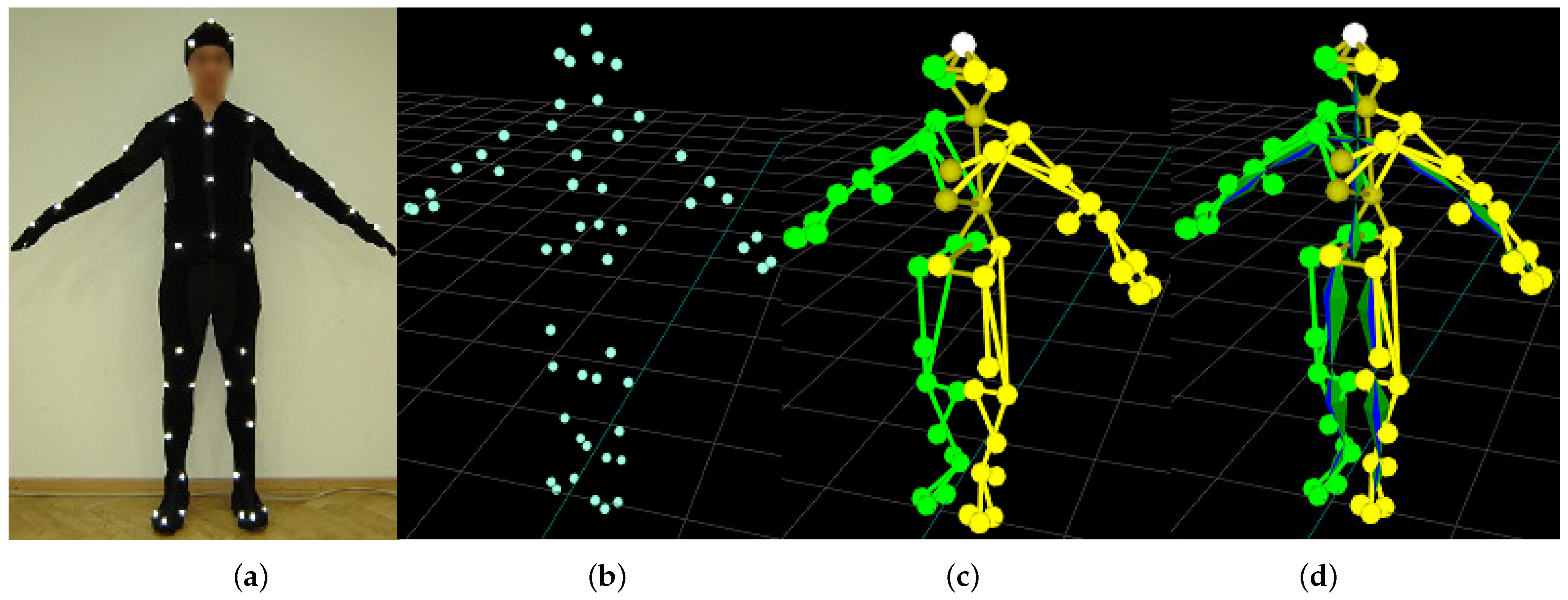
2.1. Optical Motion Capture Pipeline
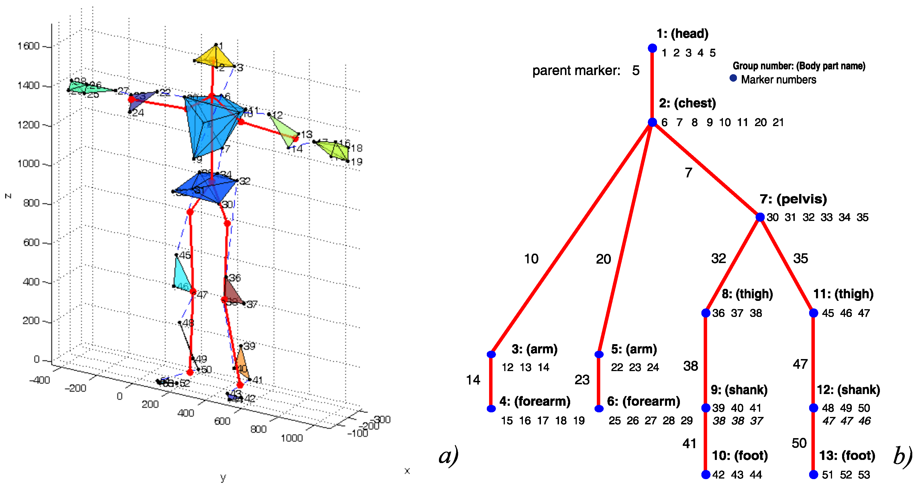
2.2. Functional Body Mesh
2.3. Previous Works
3. Materials and Methods
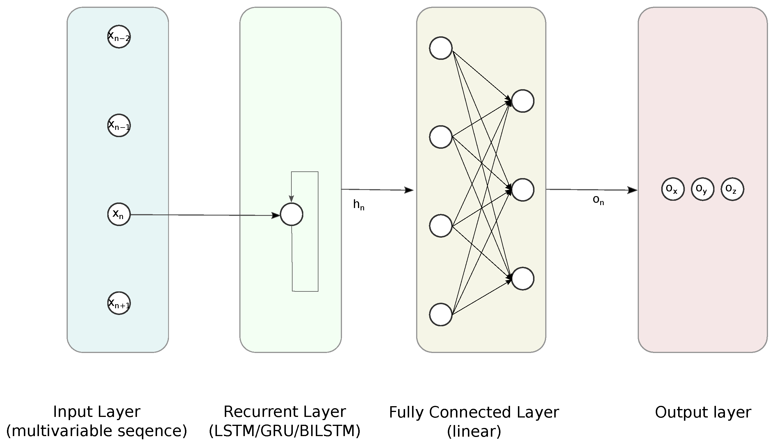
3.1. Proposed Regression Approach
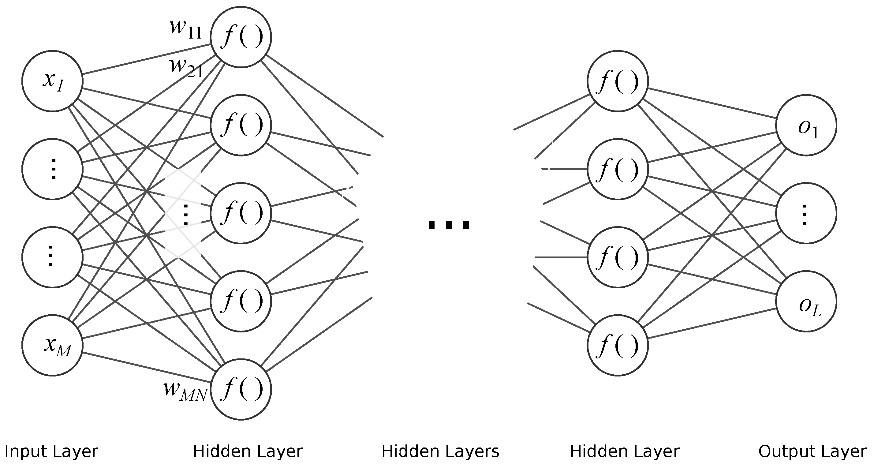
3.1.1. Feed Forward Neural Network
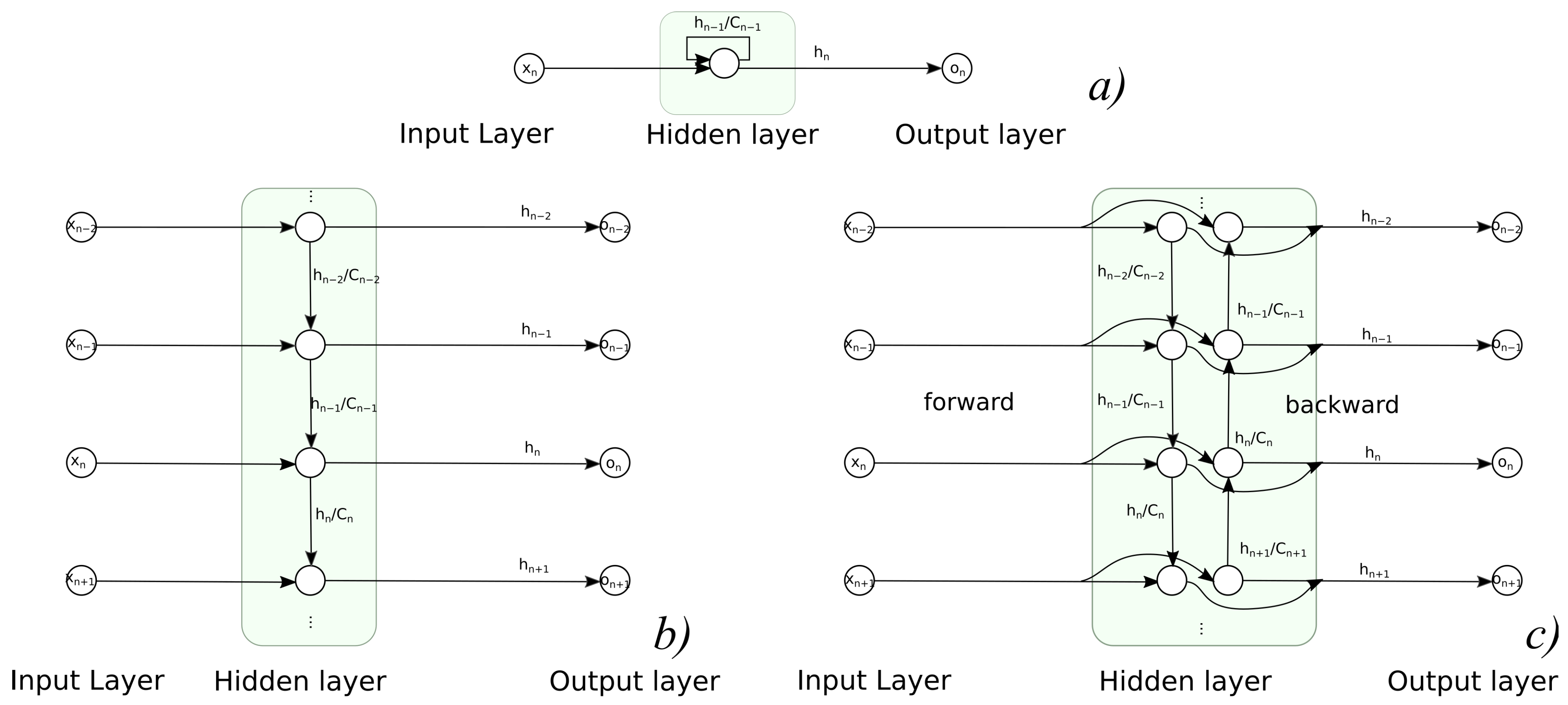
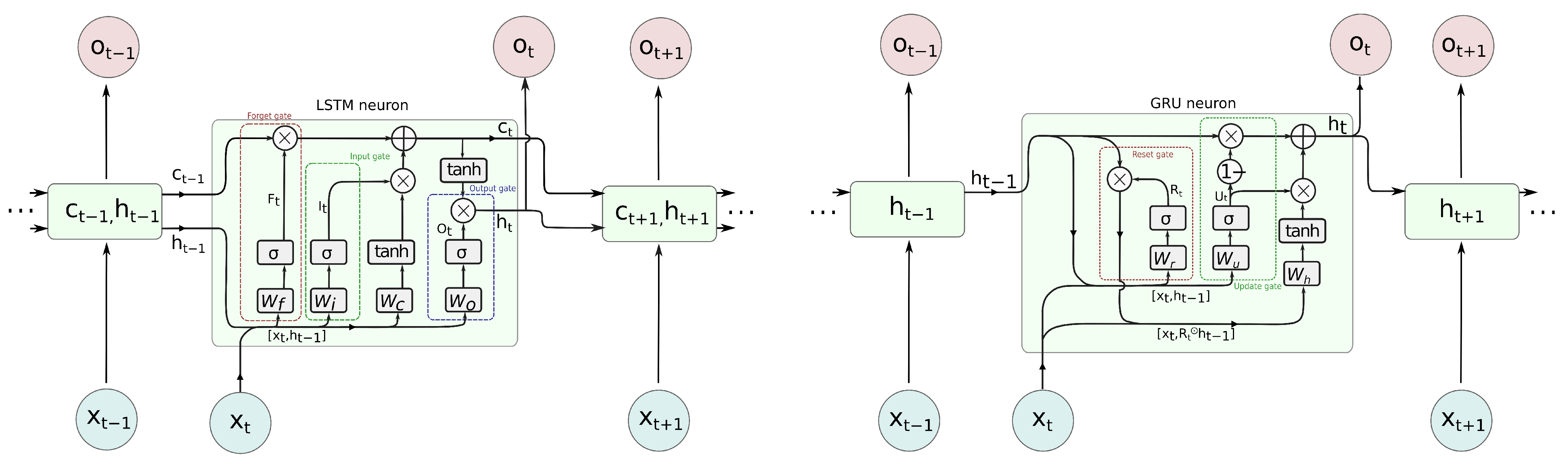
3.1.2. Recurrent Neural Networks
3.1.3. Employed Reconstruction Methods
- FFNN, with 1 hidden fully connected (FC) layer—containing 8 linear neurons;
- FFNN, with 1 hidden FC layer—containing 8 sigmoidal neurons;
- LSTM followed by 1 FC layer containing 8 sigmoidal neurons;
- GRU followed by 1 FC layer containing 8 sigmoidal neurons;
- BILSTM followed by 1 FC layer containing 8 sigmoidal neurons.
3.1.4. Implementation Details
- Initial Learn Rate: 0.01;
- Learn Rate Drop Factor: 0.9;
- Learn Rate Drop Period: 10;
- Gradient Threshold 0.7;
- Momentum: 0.8.
3.2. Input Data Preparation
3.3. Test Dataset
3.4. Quality Evaluation
3.5. Experimental Protocol
- We introduce two gaps of assumed length (on average) to the random markers at random moments; actual values are stored as testing data;
- The model is trained using the remaining part of the sequence (all but gaps);
- We reconstruct (predict) the gaps using the pool of methods;
- The resulting values are stored for evaluation.
Gap Generation Procedure
4. Results and Discussion
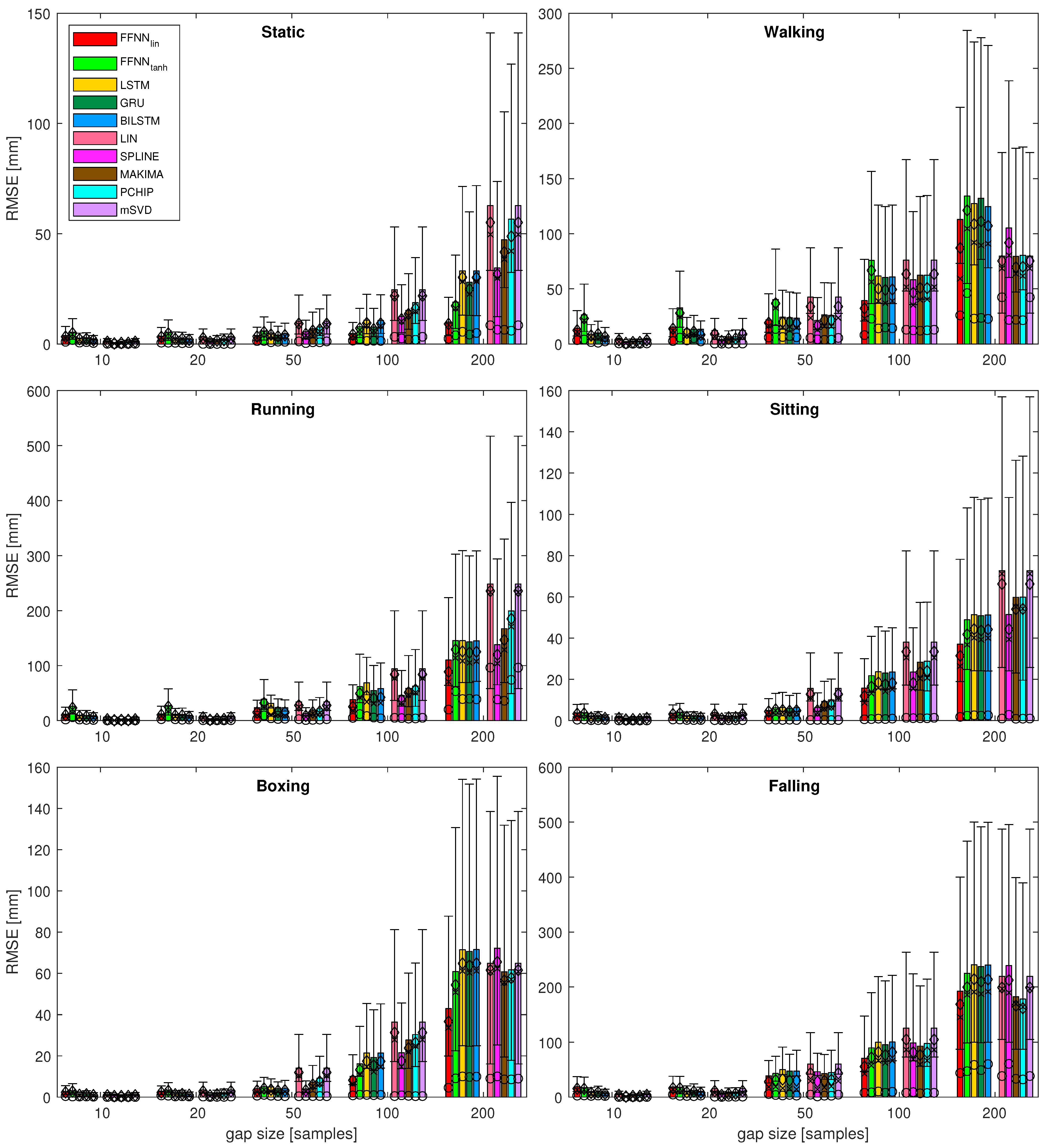
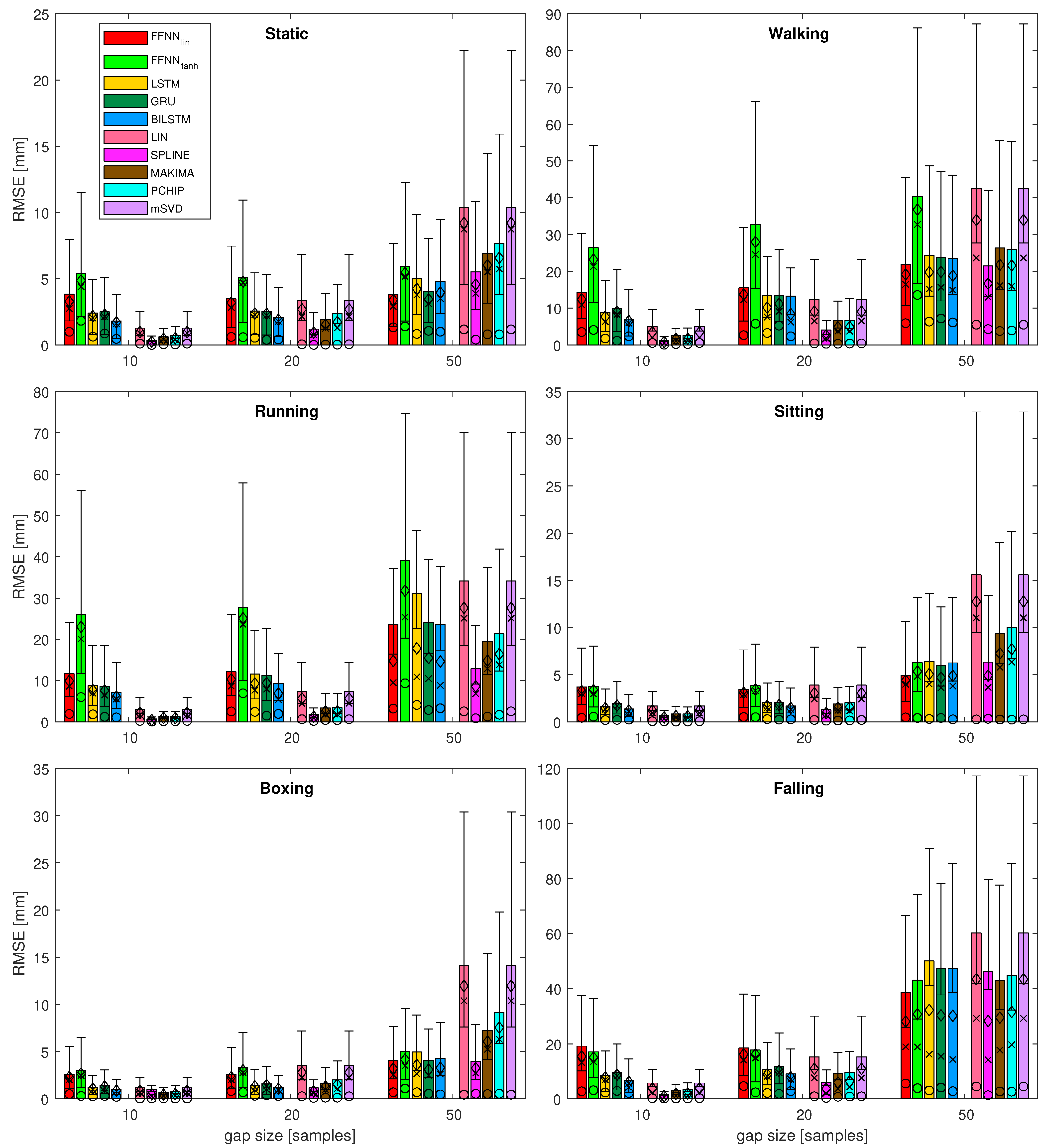
4.1. Gap Reconstruction Efficiency
- It can be seen that, for the short gaps, interpolation methods outperform any of the NN-based methods.
- For gaps that are 50 samples long, the results become less obvious and NN results are no worse or (usually) better than interpolation methods.
- Linear FFNN usually performed better than any other methods (including non-linear FFNN), for gaps of 50 samples or longer, for most of the sequences.
- In very rare cases of short-gap cases, RNNs performed better than FFNN, but, in general, simpler FFNN outperformed more complex NN models.
- There are two situations when the FFNN, performed no better or worse than interpolation methods (walking and falling). This occurred for sequences with larger monotonicity values in Table 2. They have also increased velocity/acceleration/jerk values; the ‘running’ sequence has similar values for these, but FFNN perform the best in this case, so the kinematic/dynamic parameters should not be considered.
4.2. Motion Factors Affecting Performance
5. Summary
Supplementary Materials
Author Contributions
Funding
Institutional Review Board Statement
Informed Consent Statement
Data Availability Statement
Acknowledgments
Conflicts of Interest
Abbreviations
| BILSTM | bidirectional LSTM |
| CC | correlation coefficient |
| FC | fully connected |
| FBM | functional body mesh |
| FFNN | feed forward neural network |
| GRU | gated recurrent unit |
| HML | Human Motion Laboratory |
| IK | inverse kinematics |
| KF | Kalman filter |
| LS | least squares |
| LSTM | long-short term memory |
| Mocap | MOtion CAPture |
| MSE | Mean Square Error |
| NARX-NN | nonlinear autoregressive exogenous neural network |
| NaN | not a number |
| NN | neural network |
| OMC | optical motion capture |
| PCA | principal component analysis |
| PJAIT | Polish-Japanese Academy of Information Technology |
| RMSE | root mean squared error |
| RNN | recurrent neural network |
| STDDEV | standard deviation |
| SVD | singular value decomposition |
Appendix A. Performance Results for All Sequences

| Len | FFNN | FFNN | LSTM | GRU | BILSTM | LIN | SPLINE | MAKIMA | PCHIP | mSVD | |
|---|---|---|---|---|---|---|---|---|---|---|---|
| 10 | RMSE | 14.222 | 26.428 | 8.844 | 9.932 | 7.004 | 5.088 | 1.287 | 2.464 | 2.507 | 5.088 |
| mean () | 12.398 | 23.213 | 7.659 | 9.014 | 6.495 | 3.442 | 0.810 | 1.621 | 1.697 | 3.442 | |
| median () | 10.865 | 21.290 | 6.327 | 8.262 | 5.956 | 2.051 | 0.511 | 1.087 | 1.180 | 2.051 | |
| mode () | 3.499 | 4.068 | 1.755 | 1.140 | 2.344 | 0.536 | 0.056 | 0.237 | 0.239 | 0.536 | |
| stddev () | 6.930 | 12.645 | 4.634 | 4.744 | 3.371 | 3.505 | 0.938 | 1.773 | 1.788 | 3.505 | |
| iqr () | 8.986 | 12.914 | 3.644 | 4.297 | 3.444 | 3.180 | 0.652 | 1.293 | 1.334 | 3.180 | |
| 20 | RMSE | 15.490 | 32.802 | 13.491 | 13.382 | 13.303 | 12.274 | 4.031 | 6.590 | 6.619 | 12.274 |
| mean () | 13.743 | 27.978 | 10.155 | 11.171 | 8.396 | 9.071 | 2.591 | 4.798 | 4.904 | 9.071 | |
| median () | 12.334 | 24.575 | 7.568 | 9.116 | 6.209 | 6.508 | 1.823 | 3.767 | 3.728 | 6.508 | |
| mode () | 2.654 | 5.774 | 3.242 | 5.247 | 2.352 | 0.401 | 0.314 | 0.316 | 0.382 | 0.401 | |
| stddev () | 6.723 | 16.042 | 8.161 | 6.609 | 8.827 | 8.020 | 2.828 | 4.290 | 4.175 | 8.020 | |
| iqr () | 7.454 | 15.726 | 4.545 | 5.667 | 2.491 | 6.791 | 1.571 | 3.308 | 3.921 | 6.791 | |
| 50 | RMSE | 21.907 | 40.375 | 24.343 | 23.833 | 23.434 | 42.517 | 21.474 | 26.332 | 25.995 | 42.517 |
| mean () | 19.168 | 36.769 | 19.788 | 19.867 | 18.831 | 33.944 | 16.673 | 21.757 | 21.607 | 33.944 | |
| median () | 16.432 | 32.752 | 15.196 | 15.655 | 14.926 | 23.652 | 12.952 | 16.134 | 15.996 | 23.652 | |
| mode () | 5.905 | 13.574 | 6.336 | 7.173 | 6.100 | 5.500 | 4.293 | 3.782 | 3.921 | 5.500 | |
| stddev () | 10.486 | 16.289 | 13.174 | 12.408 | 13.037 | 25.484 | 12.659 | 14.438 | 13.993 | 25.484 | |
| iqr () | 12.421 | 22.207 | 13.308 | 11.413 | 12.903 | 29.918 | 12.189 | 17.991 | 18.129 | 29.918 | |
| 100 | RMSE | 39.346 | 75.817 | 61.641 | 60.420 | 60.823 | 76.058 | 58.357 | 62.302 | 62.419 | 76.058 |
| mean () | 32.287 | 66.701 | 50.195 | 49.019 | 49.453 | 63.445 | 46.476 | 50.803 | 50.693 | 63.445 | |
| median () | 23.318 | 56.329 | 38.960 | 37.001 | 39.074 | 51.683 | 35.447 | 40.065 | 40.418 | 51.683 | |
| mode () | 8.122 | 22.940 | 14.125 | 15.094 | 14.334 | 12.943 | 12.407 | 12.074 | 12.493 | 12.943 | |
| stddev () | 22.397 | 35.709 | 35.107 | 34.707 | 34.685 | 41.564 | 34.503 | 35.371 | 35.700 | 41.564 | |
| iqr () | 18.933 | 41.446 | 39.727 | 40.427 | 40.813 | 63.062 | 39.062 | 49.784 | 50.440 | 63.062 | |
| 200 | RMSE | 112.933 | 134.121 | 127.416 | 132.150 | 124.566 | 79.741 | 105.237 | 79.407 | 80.457 | 79.741 |
| mean () | 87.084 | 121.229 | 108.733 | 111.164 | 107.192 | 75.307 | 91.826 | 69.585 | 70.031 | 75.307 | |
| median () | 59.288 | 104.710 | 91.987 | 89.523 | 91.019 | 68.567 | 80.427 | 63.559 | 61.704 | 68.567 | |
| mode () | 26.007 | 46.150 | 23.032 | 23.675 | 22.813 | 42.408 | 21.841 | 21.984 | 21.602 | 42.408 | |
| stddev () | 71.160 | 57.197 | 66.944 | 71.470 | 63.693 | 26.502 | 53.401 | 39.296 | 40.746 | 26.502 | |
| iqr () | 61.864 | 71.116 | 90.839 | 90.285 | 90.685 | 42.057 | 88.500 | 65.862 | 66.873 | 42.057 |
| Len | FFNN | FFNN | LSTM | GRU | BILSTM | LIN | SPLINE | MAKIMA | PCHIP | mSVD | |
|---|---|---|---|---|---|---|---|---|---|---|---|
| 10 | RMSE | 11.702 | 25.988 | 8.748 | 8.666 | 7.066 | 3.001 | 0.701 | 1.291 | 1.259 | 3.001 |
| mean () | 9.939 | 23.049 | 7.675 | 7.581 | 6.105 | 2.221 | 0.476 | 0.985 | 0.942 | 2.221 | |
| median () | 8.661 | 20.122 | 6.973 | 6.485 | 5.540 | 1.743 | 0.346 | 0.831 | 0.720 | 1.743 | |
| mode () | 1.933 | 6.022 | 1.838 | 1.236 | 1.106 | 0.234 | 0.079 | 0.149 | 0.151 | 0.234 | |
| stddev () | 5.919 | 11.837 | 4.214 | 4.245 | 3.797 | 1.714 | 0.439 | 0.692 | 0.691 | 1.714 | |
| iqr () | 7.005 | 15.692 | 5.106 | 4.850 | 3.513 | 1.835 | 0.286 | 0.835 | 0.799 | 1.835 | |
| 20 | RMSE | 12.141 | 27.729 | 11.594 | 11.232 | 9.321 | 7.397 | 1.742 | 3.401 | 3.439 | 7.397 |
| mean () | 10.331 | 25.124 | 9.324 | 9.440 | 6.919 | 5.676 | 1.274 | 2.601 | 2.589 | 5.676 | |
| median () | 8.695 | 23.641 | 7.664 | 7.948 | 5.424 | 4.496 | 0.968 | 1.988 | 1.853 | 4.496 | |
| mode () | 2.547 | 6.946 | 2.438 | 1.512 | 1.953 | 0.661 | 0.237 | 0.453 | 0.438 | 0.661 | |
| stddev () | 6.215 | 11.425 | 6.552 | 5.753 | 5.787 | 4.017 | 1.010 | 1.889 | 2.021 | 4.017 | |
| iqr () | 8.168 | 12.490 | 4.481 | 5.442 | 3.111 | 3.995 | 1.017 | 2.154 | 2.061 | 3.995 | |
| 50 | RMSE | 23.573 | 39.084 | 31.147 | 24.057 | 23.597 | 34.144 | 12.857 | 19.473 | 21.328 | 34.144 |
| mean () | 14.767 | 31.801 | 17.835 | 15.504 | 14.637 | 27.624 | 8.608 | 14.842 | 16.431 | 27.624 | |
| median () | 9.523 | 25.412 | 10.904 | 10.501 | 8.853 | 25.122 | 6.834 | 12.894 | 13.844 | 25.122 | |
| mode () | 3.229 | 9.379 | 4.119 | 2.888 | 3.306 | 2.559 | 0.896 | 1.291 | 1.737 | 2.559 | |
| stddev () | 18.345 | 22.596 | 25.456 | 18.049 | 18.231 | 18.865 | 8.914 | 11.837 | 12.760 | 18.865 | |
| iqr () | 6.432 | 16.838 | 6.719 | 7.811 | 7.903 | 20.224 | 6.920 | 9.883 | 11.590 | 20.224 | |
| 100 | RMSE | 38.173 | 61.656 | 68.606 | 54.639 | 58.223 | 94.347 | 45.740 | 58.606 | 62.724 | 94.347 |
| mean () | 25.165 | 49.288 | 44.780 | 40.344 | 42.251 | 83.854 | 37.303 | 51.072 | 55.958 | 83.854 | |
| median () | 18.493 | 41.944 | 33.811 | 31.168 | 32.177 | 77.220 | 32.103 | 46.438 | 50.903 | 77.220 | |
| mode () | 4.901 | 11.780 | 8.178 | 5.555 | 4.181 | 4.989 | 4.549 | 3.554 | 3.884 | 4.989 | |
| stddev () | 27.594 | 35.231 | 50.041 | 35.158 | 38.271 | 41.350 | 25.286 | 27.575 | 27.272 | 41.350 | |
| iqr () | 13.060 | 29.863 | 24.844 | 24.922 | 25.449 | 47.512 | 25.816 | 26.432 | 29.725 | 47.512 | |
| 200 | RMSE | 110.196 | 145.641 | 145.387 | 143.360 | 145.050 | 248.552 | 138.231 | 167.249 | 199.417 | 248.552 |
| mean () | 88.708 | 129.262 | 125.767 | 123.634 | 125.213 | 235.787 | 119.848 | 146.780 | 185.085 | 235.787 | |
| median () | 70.845 | 113.902 | 108.387 | 105.181 | 107.987 | 233.618 | 103.952 | 128.657 | 171.109 | 233.618 | |
| mode () | 20.092 | 53.434 | 39.113 | 39.722 | 38.728 | 96.336 | 38.444 | 36.027 | 74.145 | 96.336 | |
| stddev () | 63.969 | 65.135 | 70.990 | 70.695 | 71.285 | 73.293 | 66.963 | 77.021 | 70.628 | 73.293 | |
| iqr () | 67.200 | 73.343 | 87.747 | 82.080 | 89.947 | 77.986 | 83.010 | 64.869 | 47.085 | 77.986 |
| Len | FFNN | FFNN | LSTM | GRU | BILSTM | LIN | SPLINE | MAKIMA | PCHIP | mSVD | |
|---|---|---|---|---|---|---|---|---|---|---|---|
| 10 | RMSE | 3.701 | 3.792 | 1.664 | 1.954 | 1.373 | 1.697 | 0.711 | 0.841 | 0.839 | 1.697 |
| mean () | 3.272 | 3.386 | 1.463 | 1.737 | 1.210 | 1.218 | 0.478 | 0.617 | 0.606 | 1.218 | |
| median () | 2.996 | 2.987 | 1.351 | 1.682 | 1.108 | 0.948 | 0.339 | 0.475 | 0.429 | 0.948 | |
| mode () | 0.437 | 0.558 | 0.197 | 0.212 | 0.249 | 0.072 | 0.059 | 0.041 | 0.043 | 0.072 | |
| stddev () | 1.896 | 1.767 | 0.806 | 0.846 | 0.642 | 1.094 | 0.483 | 0.530 | 0.537 | 1.094 | |
| iqr () | 2.282 | 2.025 | 0.991 | 1.301 | 0.702 | 1.049 | 0.260 | 0.467 | 0.480 | 1.049 | |
| 20 | RMSE | 3.464 | 3.829 | 2.060 | 2.025 | 1.688 | 3.902 | 1.285 | 1.904 | 2.029 | 3.902 |
| mean () | 3.106 | 3.429 | 1.708 | 1.797 | 1.475 | 3.057 | 0.942 | 1.515 | 1.559 | 3.057 | |
| median () | 2.911 | 3.319 | 1.519 | 1.572 | 1.318 | 2.434 | 0.739 | 1.230 | 1.169 | 2.434 | |
| mode () | 0.522 | 0.497 | 0.300 | 0.240 | 0.271 | 0.211 | 0.126 | 0.155 | 0.161 | 0.211 | |
| stddev () | 1.577 | 1.750 | 1.122 | 0.962 | 0.812 | 2.415 | 0.838 | 1.153 | 1.311 | 2.415 | |
| iqr () | 2.233 | 2.263 | 1.038 | 1.069 | 0.934 | 2.762 | 0.781 | 0.979 | 0.995 | 2.762 | |
| 20 | RMSE | 4.901 | 6.291 | 6.392 | 5.952 | 6.255 | 15.596 | 6.334 | 9.332 | 10.056 | 15.596 |
| mean () | 4.383 | 5.355 | 5.064 | 4.697 | 4.895 | 12.767 | 4.902 | 7.260 | 7.710 | 12.767 | |
| median () | 3.982 | 4.831 | 4.007 | 3.623 | 3.803 | 11.036 | 3.652 | 5.788 | 6.343 | 11.036 | |
| mode () | 0.482 | 0.417 | 0.313 | 0.422 | 0.277 | 0.267 | 0.332 | 0.267 | 0.240 | 0.267 | |
| stddev () | 2.276 | 3.254 | 3.793 | 3.568 | 3.778 | 8.741 | 3.880 | 5.667 | 6.265 | 8.741 | |
| iqr () | 2.978 | 3.833 | 5.160 | 4.098 | 4.999 | 11.116 | 5.269 | 6.546 | 6.801 | 11.116 | |
| 20 | RMSE | 15.716 | 21.780 | 23.727 | 23.023 | 23.575 | 38.083 | 23.547 | 28.358 | 28.813 | 38.083 |
| mean () | 11.904 | 16.468 | 18.440 | 17.539 | 18.222 | 33.439 | 18.245 | 23.435 | 24.033 | 33.439 | |
| median () | 8.596 | 13.132 | 15.903 | 14.109 | 15.147 | 30.517 | 15.467 | 20.365 | 20.691 | 30.517 | |
| mode () | 0.643 | 0.711 | 0.927 | 0.743 | 0.950 | 1.324 | 1.170 | 1.139 | 1.121 | 1.324 | |
| stddev () | 9.980 | 13.839 | 14.495 | 14.484 | 14.524 | 17.840 | 14.459 | 15.569 | 15.542 | 17.840 | |
| iqr () | 7.816 | 11.087 | 13.380 | 12.476 | 13.201 | 23.419 | 13.054 | 15.405 | 14.280 | 23.419 | |
| 20 | RMSE | 37.101 | 48.909 | 51.388 | 50.842 | 51.274 | 72.745 | 51.478 | 59.839 | 59.857 | 72.745 |
| mean () | 31.439 | 41.811 | 44.331 | 43.711 | 44.219 | 66.280 | 44.321 | 54.030 | 54.156 | 66.280 | |
| median () | 26.422 | 36.792 | 40.178 | 39.257 | 40.099 | 71.201 | 39.395 | 55.235 | 54.311 | 71.201 | |
| mode () | 1.783 | 2.342 | 2.592 | 2.372 | 2.558 | 0.972 | 2.819 | 0.875 | 0.912 | 0.972 | |
| stddev () | 20.198 | 25.924 | 26.514 | 26.496 | 26.480 | 30.443 | 26.659 | 26.183 | 26.001 | 30.443 | |
| iqr () | 22.947 | 30.188 | 29.510 | 29.617 | 29.241 | 37.209 | 29.316 | 29.572 | 28.094 | 37.209 |
| Len | FFNN | FFNN | LSTM | GRU | BILSTM | LIN | SPLINE | MAKIMA | PCHIP | mSVD | |
|---|---|---|---|---|---|---|---|---|---|---|---|
| 10 | RMSE | 2.603 | 3.006 | 1.217 | 1.467 | 1.008 | 1.175 | 0.986 | 0.668 | 0.735 | 1.175 |
| mean () | 2.321 | 2.697 | 1.087 | 1.316 | 0.885 | 0.848 | 0.484 | 0.461 | 0.507 | 0.848 | |
| median () | 2.036 | 2.476 | 1.001 | 1.173 | 0.783 | 0.666 | 0.276 | 0.317 | 0.322 | 0.666 | |
| mode () | 0.505 | 0.309 | 0.270 | 0.303 | 0.218 | 0.036 | 0.043 | 0.035 | 0.034 | 0.036 | |
| stddev () | 1.174 | 1.354 | 0.521 | 0.613 | 0.456 | 0.712 | 0.765 | 0.420 | 0.473 | 0.712 | |
| iqr () | 1.449 | 1.769 | 0.504 | 0.705 | 0.542 | 0.709 | 0.307 | 0.341 | 0.490 | 0.709 | |
| 20 | RMSE | 2.581 | 3.298 | 1.446 | 1.591 | 1.200 | 3.534 | 1.157 | 1.648 | 2.021 | 3.534 |
| mean () | 2.295 | 3.030 | 1.341 | 1.458 | 1.070 | 2.818 | 0.797 | 1.309 | 1.519 | 2.818 | |
| median () | 2.022 | 2.780 | 1.242 | 1.353 | 0.934 | 2.282 | 0.608 | 0.983 | 1.071 | 2.282 | |
| mode () | 0.826 | 0.700 | 0.326 | 0.402 | 0.303 | 0.273 | 0.106 | 0.125 | 0.126 | 0.273 | |
| stddev () | 1.161 | 1.308 | 0.541 | 0.606 | 0.549 | 1.965 | 0.819 | 0.930 | 1.249 | 1.965 | |
| iqr () | 1.415 | 1.704 | 0.736 | 0.732 | 0.494 | 2.153 | 0.491 | 1.038 | 1.333 | 2.153 | |
| 50 | RMSE | 4.045 | 5.038 | 4.965 | 4.067 | 4.295 | 14.095 | 3.956 | 7.248 | 9.171 | 14.095 |
| mean () | 3.211 | 4.183 | 3.609 | 3.109 | 3.306 | 11.957 | 3.262 | 6.083 | 7.562 | 11.957 | |
| median () | 2.546 | 3.503 | 2.661 | 2.500 | 2.634 | 10.384 | 2.736 | 5.271 | 6.318 | 10.384 | |
| mode () | 0.699 | 1.102 | 0.699 | 0.538 | 0.480 | 0.444 | 0.542 | 0.513 | 0.546 | 0.444 | |
| stddev () | 2.460 | 2.788 | 3.404 | 2.614 | 2.747 | 7.236 | 2.235 | 3.802 | 4.994 | 7.236 | |
| iqr () | 1.743 | 1.595 | 1.968 | 1.540 | 2.062 | 9.821 | 2.059 | 5.074 | 7.302 | 9.821 | |
| 100 | RMSE | 10.134 | 16.216 | 21.424 | 19.275 | 21.386 | 36.436 | 21.538 | 27.723 | 30.374 | 36.436 |
| mean () | 8.175 | 13.241 | 17.438 | 15.384 | 17.357 | 31.336 | 17.608 | 23.779 | 26.421 | 31.336 | |
| median () | 6.398 | 11.337 | 14.702 | 12.285 | 14.627 | 27.834 | 14.823 | 22.008 | 24.825 | 27.834 | |
| mode () | 0.864 | 1.156 | 1.085 | 0.973 | 1.090 | 0.514 | 0.912 | 0.632 | 0.490 | 0.514 | |
| stddev () | 5.837 | 9.220 | 12.123 | 11.372 | 12.169 | 18.465 | 12.075 | 14.128 | 14.876 | 18.465 | |
| iqr () | 6.261 | 12.033 | 16.415 | 16.672 | 16.414 | 25.577 | 16.361 | 18.637 | 19.008 | 25.577 | |
| 200 | RMSE | 42.833 | 60.847 | 71.465 | 70.625 | 71.514 | 64.829 | 72.201 | 60.721 | 61.704 | 64.829 |
| mean () | 36.693 | 54.330 | 64.743 | 63.732 | 64.805 | 61.507 | 65.477 | 56.493 | 57.666 | 61.507 | |
| median () | 33.631 | 50.764 | 61.017 | 60.170 | 61.057 | 60.782 | 62.218 | 55.492 | 57.030 | 60.782 | |
| mode () | 4.592 | 9.116 | 10.042 | 9.788 | 9.974 | 8.998 | 10.077 | 8.616 | 8.609 | 8.998 | |
| stddev () | 21.768 | 26.954 | 29.620 | 29.819 | 29.609 | 20.171 | 29.798 | 22.097 | 21.740 | 20.171 | |
| iqr () | 21.992 | 31.408 | 36.039 | 35.205 | 36.075 | 24.945 | 36.485 | 29.814 | 28.505 | 24.945 |
| Len | FFNN | FFNN | LSTM | GRU | BILSTM | LIN | SPLINE | MAKIMA | PCHIP | mSVD | |
|---|---|---|---|---|---|---|---|---|---|---|---|
| 10 | RMSE | 19.193 | 17.106 | 8.537 | 9.585 | 6.720 | 5.763 | 1.601 | 2.872 | 3.365 | 5.763 |
| mean () | 15.455 | 15.022 | 7.818 | 8.772 | 6.166 | 3.827 | 0.994 | 1.851 | 1.968 | 3.827 | |
| median () | 13.186 | 13.571 | 6.947 | 8.341 | 5.616 | 2.359 | 0.618 | 1.107 | 1.145 | 2.359 | |
| mode () | 2.760 | 3.139 | 2.310 | 2.880 | 2.110 | 0.244 | 0.105 | 0.145 | 0.149 | 0.244 | |
| stddev () | 11.270 | 8.163 | 3.494 | 3.852 | 2.555 | 4.023 | 1.138 | 2.039 | 2.551 | 4.023 | |
| iqr () | 9.203 | 10.174 | 3.101 | 4.009 | 3.520 | 3.723 | 0.789 | 1.795 | 1.813 | 3.723 | |
| 20 | RMSE | 18.496 | 17.762 | 10.664 | 11.914 | 9.057 | 15.278 | 6.073 | 9.213 | 9.596 | 15.278 |
| mean () | 16.206 | 16.199 | 8.940 | 10.261 | 7.897 | 10.937 | 3.694 | 5.981 | 6.392 | 10.937 | |
| median () | 14.108 | 14.897 | 8.130 | 9.530 | 7.106 | 7.613 | 2.089 | 3.687 | 4.319 | 7.613 | |
| mode () | 4.659 | 2.388 | 2.143 | 1.822 | 2.821 | 0.953 | 0.339 | 0.756 | 0.832 | 0.953 | |
| stddev () | 8.511 | 7.184 | 6.211 | 5.915 | 4.455 | 9.596 | 4.383 | 6.169 | 6.567 | 9.596 | |
| iqr () | 9.496 | 8.219 | 4.321 | 5.520 | 3.642 | 10.133 | 3.402 | 5.298 | 5.154 | 10.133 | |
| 50 | RMSE | 38.618 | 43.058 | 50.077 | 47.367 | 47.474 | 60.232 | 46.220 | 42.945 | 44.782 | 60.232 |
| mean () | 28.149 | 30.795 | 32.292 | 30.356 | 30.213 | 43.423 | 28.314 | 29.543 | 31.603 | 43.423 | |
| median () | 18.927 | 18.873 | 16.214 | 15.491 | 14.312 | 29.262 | 14.172 | 17.724 | 19.705 | 29.262 | |
| mode () | 5.585 | 3.883 | 3.061 | 4.112 | 2.789 | 4.507 | 1.345 | 2.710 | 2.615 | 4.507 | |
| stddev () | 25.916 | 29.395 | 37.233 | 35.345 | 35.587 | 42.053 | 35.660 | 31.333 | 31.914 | 42.053 | |
| iqr () | 15.417 | 17.126 | 31.871 | 21.094 | 29.043 | 38.828 | 27.009 | 24.239 | 28.168 | 38.828 | |
| 100 | RMSE | 70.671 | 89.650 | 100.005 | 95.523 | 100.282 | 125.495 | 98.770 | 92.878 | 97.573 | 125.495 |
| mean () | 55.641 | 72.172 | 81.983 | 76.503 | 81.814 | 104.667 | 81.794 | 76.620 | 81.261 | 104.667 | |
| median () | 42.728 | 57.532 | 66.468 | 62.277 | 66.311 | 86.119 | 68.990 | 59.710 | 66.757 | 86.119 | |
| mode () | 7.967 | 8.688 | 10.247 | 7.912 | 9.749 | 7.809 | 9.146 | 6.892 | 7.449 | 7.809 | |
| stddev () | 43.593 | 53.283 | 57.286 | 57.268 | 58.033 | 69.796 | 55.712 | 52.857 | 54.185 | 69.796 | |
| iqr () | 52.533 | 72.029 | 82.980 | 85.218 | 86.618 | 85.060 | 92.529 | 71.859 | 75.211 | 85.060 | |
| 200 | RMSE | 192.371 | 224.989 | 240.459 | 237.068 | 240.104 | 219.332 | 238.962 | 182.390 | 177.973 | 219.332 |
| mean () | 168.542 | 199.701 | 214.118 | 209.626 | 213.731 | 198.998 | 212.497 | 165.908 | 161.330 | 198.998 | |
| median () | 145.399 | 185.636 | 190.954 | 187.446 | 191.565 | 196.704 | 189.560 | 169.458 | 163.676 | 196.704 | |
| mode () | 43.924 | 47.226 | 58.636 | 49.156 | 60.128 | 38.386 | 60.706 | 33.396 | 32.207 | 38.386 | |
| stddev () | 92.157 | 103.406 | 108.703 | 110.129 | 108.684 | 94.898 | 108.542 | 77.915 | 77.491 | 94.898 | |
| iqr () | 102.432 | 114.007 | 119.186 | 116.515 | 119.440 | 153.708 | 117.857 | 121.289 | 120.480 | 153.708 |
Appendix B. Correlations between RMSE an Sequence Parameters
| Len | FFNN | FFNN | LSTM | GRU | BILSTM | LIN | SPLINE | MAKIMA | PCHIP | mSVD |
|---|---|---|---|---|---|---|---|---|---|---|
| 10 | 0.741 | 0.878 | 0.890 | 0.849 | 0.890 | 0.614 | 0.261 | 0.552 | 0.520 | 0.614 |
| 20 | 0.760 | 0.827 | 0.852 | 0.842 | 0.790 | 0.608 | 0.466 | 0.550 | 0.533 | 0.608 |
| 50 | 0.744 | 0.851 | 0.740 | 0.678 | 0.670 | 0.660 | 0.503 | 0.603 | 0.608 | 0.660 |
| 100 | 0.639 | 0.719 | 0.724 | 0.649 | 0.662 | 0.742 | 0.576 | 0.661 | 0.679 | 0.742 |
| 200 | 0.658 | 0.691 | 0.667 | 0.665 | 0.664 | 0.777 | 0.626 | 0.756 | 0.812 | 0.777 |
| 10 | 0.092 | 0.021 | 0.017 | 0.033 | 0.017 | 0.195 | 0.617 | 0.256 | 0.290 | 0.195 |
| 20 | 0.080 | 0.042 | 0.031 | 0.036 | 0.061 | 0.200 | 0.352 | 0.258 | 0.276 | 0.200 |
| 50 | 0.090 | 0.032 | 0.093 | 0.139 | 0.146 | 0.153 | 0.309 | 0.205 | 0.200 | 0.153 |
| 100 | 0.172 | 0.108 | 0.104 | 0.163 | 0.152 | 0.091 | 0.231 | 0.153 | 0.138 | 0.091 |
| 200 | 0.155 | 0.129 | 0.148 | 0.150 | 0.150 | 0.069 | 0.184 | 0.082 | 0.050 | 0.069 |
| Len | FFNN | FFNN | LSTM | GRU | BILSTM | LIN | SPLINE | MAKIMA | PCHIP | mSVD |
|---|---|---|---|---|---|---|---|---|---|---|
| 10 | 0.775 | 0.997 | 0.950 | 0.928 | 0.956 | 0.729 | 0.419 | 0.668 | 0.586 | 0.729 |
| 20 | 0.823 | 0.986 | 0.969 | 0.943 | 0.948 | 0.688 | 0.505 | 0.595 | 0.556 | 0.688 |
| 50 | 0.736 | 0.924 | 0.703 | 0.661 | 0.645 | 0.718 | 0.479 | 0.627 | 0.614 | 0.718 |
| 100 | 0.673 | 0.833 | 0.755 | 0.708 | 0.698 | 0.747 | 0.611 | 0.718 | 0.707 | 0.747 |
| 200 | 0.696 | 0.719 | 0.649 | 0.667 | 0.641 | 0.648 | 0.570 | 0.659 | 0.694 | 0.648 |
| 10 | 0.070 | 0.000 | 0.004 | 0.007 | 0.003 | 0.100 | 0.408 | 0.147 | 0.222 | 0.100 |
| 20 | 0.044 | 0.000 | 0.001 | 0.005 | 0.004 | 0.131 | 0.307 | 0.213 | 0.252 | 0.131 |
| 50 | 0.095 | 0.008 | 0.119 | 0.153 | 0.167 | 0.108 | 0.336 | 0.183 | 0.195 | 0.108 |
| 100 | 0.143 | 0.040 | 0.083 | 0.115 | 0.123 | 0.088 | 0.198 | 0.108 | 0.116 | 0.088 |
| 200 | 0.125 | 0.107 | 0.163 | 0.148 | 0.170 | 0.164 | 0.237 | 0.155 | 0.126 | 0.164 |
| Len | FFNN | FFNN | LSTM | GRU | BILSTM | LIN | SPLINE | MAKIMA | PCHIP | mSVD |
|---|---|---|---|---|---|---|---|---|---|---|
| 10 | 0.768 | 0.983 | 0.943 | 0.915 | 0.950 | 0.701 | 0.419 | 0.640 | 0.564 | 0.701 |
| 20 | 0.812 | 0.962 | 0.950 | 0.927 | 0.916 | 0.669 | 0.486 | 0.576 | 0.540 | 0.669 |
| 50 | 0.749 | 0.921 | 0.724 | 0.672 | 0.657 | 0.716 | 0.478 | 0.624 | 0.619 | 0.716 |
| 100 | 0.681 | 0.825 | 0.772 | 0.715 | 0.709 | 0.771 | 0.615 | 0.728 | 0.723 | 0.771 |
| 200 | 0.712 | 0.742 | 0.679 | 0.694 | 0.673 | 0.710 | 0.609 | 0.714 | 0.755 | 0.710 |
| 10 | 0.074 | 0.000 | 0.005 | 0.011 | 0.004 | 0.121 | 0.409 | 0.172 | 0.243 | 0.121 |
| 20 | 0.050 | 0.002 | 0.004 | 0.008 | 0.010 | 0.146 | 0.328 | 0.231 | 0.269 | 0.146 |
| 50 | 0.087 | 0.009 | 0.104 | 0.143 | 0.157 | 0.110 | 0.338 | 0.186 | 0.190 | 0.110 |
| 100 | 0.136 | 0.043 | 0.072 | 0.111 | 0.115 | 0.072 | 0.194 | 0.101 | 0.104 | 0.072 |
| 200 | 0.112 | 0.091 | 0.138 | 0.126 | 0.143 | 0.114 | 0.199 | 0.111 | 0.083 | 0.114 |
| Len | FFNN | FFNN | LSTM | GRU | BILSTM | LIN | SPLINE | MAKIMA | PCHIP | mSVD |
|---|---|---|---|---|---|---|---|---|---|---|
| 10 | 0.901 | 0.867 | 0.917 | 0.928 | 0.922 | 0.879 | 0.775 | 0.853 | 0.806 | 0.879 |
| 20 | 0.923 | 0.853 | 0.916 | 0.932 | 0.894 | 0.870 | 0.754 | 0.806 | 0.779 | 0.870 |
| 50 | 0.896 | 0.952 | 0.870 | 0.858 | 0.846 | 0.909 | 0.740 | 0.845 | 0.844 | 0.909 |
| 100 | 0.886 | 0.960 | 0.928 | 0.916 | 0.907 | 0.914 | 0.858 | 0.926 | 0.916 | 0.914 |
| 200 | 0.918 | 0.929 | 0.884 | 0.901 | 0.879 | 0.699 | 0.830 | 0.789 | 0.745 | 0.699 |
| 10 | 0.014 | 0.025 | 0.010 | 0.008 | 0.009 | 0.021 | 0.070 | 0.031 | 0.053 | 0.021 |
| 20 | 0.009 | 0.031 | 0.010 | 0.007 | 0.016 | 0.024 | 0.083 | 0.053 | 0.068 | 0.024 |
| 50 | 0.016 | 0.003 | 0.024 | 0.029 | 0.034 | 0.012 | 0.093 | 0.034 | 0.034 | 0.012 |
| 100 | 0.019 | 0.002 | 0.008 | 0.010 | 0.012 | 0.011 | 0.029 | 0.008 | 0.010 | 0.011 |
| 200 | 0.010 | 0.007 | 0.019 | 0.014 | 0.021 | 0.122 | 0.041 | 0.062 | 0.089 | 0.122 |
| Len | FFNN | FFNN | LSTM | GRU | BILSTM | LIN | SPLINE | MAKIMA | PCHIP | mSVD |
|---|---|---|---|---|---|---|---|---|---|---|
| 10 | 0.784 | 0.711 | 0.752 | 0.785 | 0.760 | 0.823 | 0.861 | 0.818 | 0.765 | 0.823 |
| 20 | 0.811 | 0.723 | 0.778 | 0.798 | 0.784 | 0.810 | 0.720 | 0.750 | 0.720 | 0.810 |
| 50 | 0.772 | 0.813 | 0.736 | 0.749 | 0.737 | 0.833 | 0.674 | 0.770 | 0.766 | 0.833 |
| 100 | 0.806 | 0.881 | 0.826 | 0.846 | 0.827 | 0.797 | 0.800 | 0.855 | 0.830 | 0.797 |
| 200 | 0.843 | 0.843 | 0.791 | 0.816 | 0.785 | 0.502 | 0.736 | 0.625 | 0.546 | 0.502 |
| 10 | 0.065 | 0.113 | 0.084 | 0.064 | 0.080 | 0.044 | 0.028 | 0.047 | 0.076 | 0.044 |
| 20 | 0.050 | 0.104 | 0.068 | 0.057 | 0.065 | 0.051 | 0.107 | 0.086 | 0.106 | 0.051 |
| 50 | 0.072 | 0.049 | 0.095 | 0.086 | 0.095 | 0.040 | 0.142 | 0.073 | 0.076 | 0.040 |
| 100 | 0.053 | 0.020 | 0.043 | 0.034 | 0.042 | 0.057 | 0.056 | 0.030 | 0.041 | 0.057 |
| 200 | 0.035 | 0.035 | 0.061 | 0.048 | 0.064 | 0.311 | 0.095 | 0.185 | 0.262 | 0.311 |
| Len | FFNN | FFNN | LSTM | GRU | BILSTM | LIN | SPLINE | MAKIMA | PCHIP | mSVD |
|---|---|---|---|---|---|---|---|---|---|---|
| 10 | 0.918 | 0.533 | 0.722 | 0.781 | 0.709 | 0.952 | 0.866 | 0.971 | 0.993 | 0.952 |
| 20 | 0.898 | 0.529 | 0.694 | 0.759 | 0.703 | 0.971 | 0.999 | 0.993 | 0.996 | 0.971 |
| 50 | 0.883 | 0.774 | 0.857 | 0.914 | 0.918 | 0.937 | 0.974 | 0.965 | 0.953 | 0.937 |
| 100 | 0.908 | 0.873 | 0.853 | 0.908 | 0.904 | 0.817 | 0.951 | 0.897 | 0.890 | 0.817 |
| 200 | 0.892 | 0.858 | 0.866 | 0.871 | 0.862 | 0.441 | 0.842 | 0.612 | 0.476 | 0.441 |
| 10 | 0.010 | 0.276 | 0.106 | 0.067 | 0.115 | 0.003 | 0.026 | 0.001 | 0.000 | 0.003 |
| 20 | 0.015 | 0.281 | 0.126 | 0.080 | 0.119 | 0.001 | 0.000 | 0.000 | 0.000 | 0.001 |
| 50 | 0.020 | 0.071 | 0.029 | 0.011 | 0.010 | 0.006 | 0.001 | 0.002 | 0.003 | 0.006 |
| 100 | 0.012 | 0.023 | 0.031 | 0.012 | 0.013 | 0.047 | 0.003 | 0.015 | 0.018 | 0.047 |
| 200 | 0.017 | 0.029 | 0.026 | 0.024 | 0.027 | 0.381 | 0.036 | 0.196 | 0.340 | 0.381 |
| Len | FFNN | FFNN | LSTM | GRU | BILSTM | LIN | SPLINE | MAKIMA | PCHIP | mSVD |
|---|---|---|---|---|---|---|---|---|---|---|
| 10 | −0.795 | −0.937 | −0.913 | −0.906 | −0.922 | −0.781 | −0.532 | −0.729 | −0.645 | −0.781 |
| 20 | −0.837 | −0.931 | −0.936 | −0.920 | −0.919 | −0.733 | −0.568 | −0.644 | −0.599 | −0.733 |
| 50 | −0.763 | −0.914 | −0.730 | −0.703 | −0.687 | −0.770 | −0.544 | −0.685 | −0.670 | −0.770 |
| 100 | −0.744 | −0.878 | −0.802 | −0.775 | −0.758 | −0.787 | −0.682 | −0.780 | −0.759 | −0.787 |
| 200 | −0.754 | −0.769 | −0.692 | −0.714 | −0.685 | −0.637 | −0.618 | −0.673 | −0.675 | −0.637 |
| 10 | 0.059 | 0.006 | 0.011 | 0.013 | 0.009 | 0.067 | 0.278 | 0.100 | 0.167 | 0.067 |
| 20 | 0.038 | 0.007 | 0.006 | 0.009 | 0.010 | 0.097 | 0.239 | 0.167 | 0.209 | 0.097 |
| 50 | 0.078 | 0.011 | 0.099 | 0.119 | 0.131 | 0.074 | 0.265 | 0.134 | 0.145 | 0.074 |
| 100 | 0.090 | 0.021 | 0.055 | 0.070 | 0.081 | 0.063 | 0.135 | 0.067 | 0.080 | 0.063 |
| 200 | 0.083 | 0.074 | 0.128 | 0.111 | 0.133 | 0.174 | 0.191 | 0.143 | 0.141 | 0.174 |
References
- Kitagawa, M.; Windsor, B. MoCap for Artists: Workflow and Techniques for Motion Capture; Elsevier: Amsterdam, The Netherlands; Focal Press: Boston, MA, USA, 2008. [Google Scholar]
- Menache, A. Understanding Motion Capture for Computer Animation, 2nd ed.; Morgan Kaufmann: Burlington, MA, USA, 2011. [Google Scholar]
- Mündermann, L.; Corazza, S.; Andriacchi, T.P. The evolution of methods for the capture of human movement leading to markerless motion capture for biomechanical applications. J. Neuroeng. Rehabil. 2006, 3, 6. [Google Scholar] [CrossRef] [PubMed]
- Szczęsna, A.; Błaszczyszyn, M.; Pawlyta, M. Optical motion capture dataset of selected techniques in beginner and advanced Kyokushin karate athletes. Sci. Data 2021, 8, 13. [Google Scholar] [CrossRef] [PubMed]
- Świtoński, A.; Mucha, R.; Danowski, D.; Mucha, M.; Polański, A.; Cieślar, G.; Wojciechowski, K.; Sieroń, A. Diagnosis of the motion pathologies based on a reduced kinematical data of a gait. PrzegląD Elektrotechniczny 2011, 87, 173–176. [Google Scholar]
- Lachor, M.; Świtoński, A.; Boczarska-Jedynak, M.; Kwiek, S.; Wojciechowski, K.; Polański, A. The Analysis of Correlation between MOCAP-Based and UPDRS-Based Evaluation of Gait in Parkinson’s Disease Patients. In Brain Informatics and Health; Ślęzak, D., Tan, A.H., Peters, J.F., Schwabe, L., Eds.; Number 8609 in Lecture Notes in Computer Science; Springer International Publishing: Cham, Switzerland, 2014; pp. 335–344. [Google Scholar] [CrossRef]
- Josinski, H.; Świtoński, A.; Stawarz, M.; Mucha, R.; Wojciechowski, K. Evaluation of rehabilitation progress of patients with osteoarthritis of the hip, osteoarthritis of the spine or after stroke using gait indices. Przegląd Elektrotechniczny 2013, 89, 279–282. [Google Scholar]
- Windolf, M.; Götzen, N.; Morlock, M. Systematic accuracy and precision analysis of video motion capturing systems—Exemplified on the Vicon-460 system. J. Biomech. 2008, 41, 2776–2780. [Google Scholar] [CrossRef]
- Jensenius, A.; Nymoen, K.; Skogstad, S.; Voldsund, A. A Study of the Noise-Level in Two Infrared Marker-Based Motion Capture Systems. In Proceedings of the 9th Sound and Music Computing Conference, SMC 2012, Copenhagen, Denmark, 11–14 July 2012; pp. 258–263. [Google Scholar]
- Skurowski, P.; Pawlyta, M. On the Noise Complexity in an Optical Motion Capture Facility. Sensors 2019, 19, 4435. [Google Scholar] [CrossRef] [PubMed]
- Skurowski, P.; Pawlyta, M. Functional Body Mesh Representation, A Simplified Kinematic Model, Its Inference and Applications. Appl. Math. Inf. Sci. 2016, 10, 71–82. [Google Scholar] [CrossRef]
- Herda, L.; Fua, P.; Plankers, R.; Boulic, R.; Thalmann, D. Skeleton-based motion capture for robust reconstruction of human motion. In Proceedings of the Proceedings Computer Animation 2000, Philadelphia, PA, USA, 3–5 May 2000; pp. 77–83, ISSN: 1087-4844. [Google Scholar] [CrossRef]
- Aristidou, A.; Lasenby, J. Real-time marker prediction and CoR estimation in optical motion capture. Vis. Comput. 2013, 29, 7–26. [Google Scholar] [CrossRef]
- Perepichka, M.; Holden, D.; Mudur, S.P.; Popa, T. Robust Marker Trajectory Repair for MOCAP using Kinematic Reference. In Motion, Interaction and Games; Association for Computing Machinery: New York, NY, USA, 2019; MIG’19; pp. 1–10. [Google Scholar] [CrossRef]
- Lee, J.; Shin, S.Y. A hierarchical approach to interactive motion editing for human-like figures. In Proceedings of the 26th Annual Conference on Computer Graphics and Interactive Techniques, Los Angeles, CA, USA, 8–13 August 1999; ACM Press/Addison-Wesley Publishing Co.: New York, NY, USA, 1999; pp. 39–48. [Google Scholar] [CrossRef]
- Howarth, S.J.; Callaghan, J.P. Quantitative assessment of the accuracy for three interpolation techniques in kinematic analysis of human movement. Comput. Methods Biomech. Biomed. Eng. 2010, 13, 847–855. [Google Scholar] [CrossRef]
- Reda, H.E.A.; Benaoumeur, I.; Kamel, B.; Zoubir, A.F. MoCap systems and hand movement reconstruction using cubic spline. In Proceedings of the 2018 5th International Conference on Control, Decision and Information Technologies (CoDIT), Thessaloniki, Greece, 10–13 April 2018; pp. 1–5. [Google Scholar] [CrossRef]
- Liu, G.; McMillan, L. Estimation of missing markers in human motion capture. Vis. Comput. 2006, 22, 721–728. [Google Scholar] [CrossRef]
- Lai, R.Y.Q.; Yuen, P.C.; Lee, K.K.W. Motion Capture Data Completion and Denoising by Singular Value Thresholding. In Eurographics 2011—Short Papers; Avis, N., Lefebvre, S., Eds.; The Eurographics Association: Geneve, Switzerland, 2011. [Google Scholar] [CrossRef]
- Gløersen, Ø.; Federolf, P. Predicting Missing Marker Trajectories in Human Motion Data Using Marker Intercorrelations. PLoS ONE 2016, 11, e0152616. [Google Scholar] [CrossRef]
- Tits, M.; Tilmanne, J.; Dutoit, T. Robust and automatic motion-capture data recovery using soft skeleton constraints and model averaging. PLoS ONE 2018, 13, e0199744. [Google Scholar] [CrossRef]
- Piazza, T.; Lundström, J.; Kunz, A.; Fjeld, M. Predicting Missing Markers in Real-Time Optical Motion Capture. In Modelling the Physiological Human; Magnenat-Thalmann, N., Ed.; Number 5903 in Lecture Notes in Computer Science; Springer: Berlin/Heidelberg, Germany, 2009; pp. 125–136. [Google Scholar]
- Wu, Q.; Boulanger, P. Real-Time Estimation of Missing Markers for Reconstruction of Human Motion. In Proceedings of the 2011 XIII Symposium on Virtual Reality, Uberlandia, Brazil, 23–26 May 2011; pp. 161–168. [Google Scholar] [CrossRef]
- Li, L.; McCann, J.; Pollard, N.S.; Faloutsos, C. DynaMMo: Mining and summarization of coevolving sequences with missing values. In Proceedings of the 15th ACM SIGKDD International Conference on Knowledge Discovery and Data Mining; Association for Computing Machinery: New York, NY, USA, 2009; pp. 507–516. [Google Scholar] [CrossRef]
- Li, L.; McCann, J.; Pollard, N.; Faloutsos, C. BoLeRO: A Principled Technique for Including Bone Length Constraints in Motion Capture Occlusion Filling. In Proceedings of the 2010 ACM SIGGRAPH/Eurographics Symposium on Computer Animation; Eurographics Association: Aire-la-Ville, Switzerland, 2010; pp. 179–188. [Google Scholar]
- Burke, M.; Lasenby, J. Estimating missing marker positions using low dimensional Kalman smoothing. J. Biomech. 2016, 49, 1854–1858. [Google Scholar] [CrossRef]
- Wang, Z.; Liu, S.; Qian, R.; Jiang, T.; Yang, X.; Zhang, J.J. Human motion data refinement unitizing structural sparsity and spatial-temporal information. In Proceedings of the IEEE 13th International Conference on Signal Processing (ICSP), Chengdu, China, 6–10 November 2017; pp. 975–982. [Google Scholar]
- Aristidou, A.; Cohen-Or, D.; Hodgins, J.K.; Shamir, A. Self-similarity Analysis for Motion Capture Cleaning. Comput. Graph. Forum 2018, 37, 297–309. [Google Scholar] [CrossRef]
- Zhang, X.; van de Panne, M. Data-driven autocompletion for keyframe animation. In Proceedings of the 11th Annual International Conference on Motion, Interaction, and Games, New York, NY, USA, 8–10 November 2018; Association for Computing Machinery: New York, NY, USA, 2018; pp. 1–11. [Google Scholar] [CrossRef]
- Hornik, K. Approximation capabilities of multilayer feedforward networks. Neural Netw. 1991, 4, 251–257. [Google Scholar] [CrossRef]
- Fragkiadaki, K.; Levine, S.; Felsen, P.; Malik, J. Recurrent Network Models for Human Dynamics. In Proceedings of the 2015 IEEE International Conference on Computer Vision (ICCV), Santiago, Chile, 7–13 December 2015; pp. 4346–4354, ISSN: 2380-7504. [Google Scholar] [CrossRef]
- Harvey, F.G.; Yurick, M.; Nowrouzezahrai, D.; Pal, C. Robust motion in-betweening. ACM Trans. Graph. 2020, 39, 60:60:1–60:60:12. [Google Scholar] [CrossRef]
- Mall, U.; Lal, G.R.; Chaudhuri, S.; Chaudhuri, P. A Deep Recurrent Framework for Cleaning Motion Capture Data. arXiv 2017, arXiv:1712.03380. [Google Scholar]
- Kucherenko, T.; Beskow, J.; Kjellström, H. A Neural Network Approach to Missing Marker Reconstruction in Human Motion Capture. arXiv 2018, arXiv:1803.02665. [Google Scholar]
- Holden, D. Robust solving of optical motion capture data by denoising. ACM Trans. Graph. 2018, 37, 165:1–165:12. [Google Scholar] [CrossRef]
- Ji, L.; Liu, R.; Zhou, D.; Zhang, Q.; Wei, X. Missing Data Recovery for Human Mocap Data Based on A-LSTM and LS Constraint. In Proceedings of the 2020 IEEE 5th International Conference on Signal and Image Processing (ICSIP), Nanjing, China, 23–25 October 2020; pp. 729–734. [Google Scholar] [CrossRef]
- Kaufmann, M.; Aksan, E.; Song, J.; Pece, F.; Ziegler, R.; Hilliges, O. Convolutional Autoencoders for Human Motion Infilling. arXiv 2020, arXiv:2010.11531. [Google Scholar]
- Torres, J.F.; Hadjout, D.; Sebaa, A.; Martínez-Álvarez, F.; Troncoso, A. Deep Learning for Time Series Forecasting: A Survey. Big Data 2021, 9, 3–21. [Google Scholar] [CrossRef] [PubMed]
- Shahid, F.; Zameer, A.; Muneeb, M. Predictions for COVID-19 with deep learning models of LSTM, GRU and Bi-LSTM. Chaos Solitons Fractals 2020, 140, 110212. [Google Scholar] [CrossRef] [PubMed]
- Siami-Namini, S.; Tavakoli, N.; Namin, A.S. The Performance of LSTM and BiLSTM in Forecasting Time Series. In Proceedings of the 2019 IEEE International Conference on Big Data (Big Data), Los Angeles, CA, USA, 9–12 December 2019; pp. 3285–3292. [Google Scholar] [CrossRef]
- Czekalski, P.; Łyp, K. Neural network structure optimization in pattern recognition. Stud. Inform. 2014, 35, 17–32. [Google Scholar]
- Srebro, N.; Jaakkola, T. Weighted low-rank approximations. In Proceedings of the Twentieth International Conference on International Conference on Machine Learning, Washington, DC, USA, 21–24 August 2003; AAAI Press: Washington, DC, USA, 2003; pp. 720–727. [Google Scholar]
| No. | Name | Scenario | Duration | Difficulty |
|---|---|---|---|---|
| 1 | Static | Actor stands in the middle of scene, looking around and shifting from one foot to another, freely swinging arms | 32 s | varied motions |
| 2 | Walking | Actor stands still at the edge of the scene, then walks straight for 6 m, then stands still | 7 s | low dynamics, easy |
| 3 | Running | Actor stands in the middle of scene, then goes backwards to the edge of the scene and runs for 6 m, then goes backwards to the middle of the scene | 16 s | moderate dynamics |
| 4 | Sitting | Actor stands in the middle of scene, then sits on a stool, and, after a few seconds, stands again | 15 s | occlusions |
| 5 | Boxing | Actor stands in the middle of scene, and performs some fast boxing punches | 14 s | high dynamics |
| 6 | Falling | Actor stands on 0.5 m elevation in the middle of scene, the walks to edge of platform, then falls on the mattress, lies for 2 s and stands | 16 s | high dynamics, occlusions |
| No | Entropy () | Stddev () | Velocity () | Acc. () | Jerk () | Monotonicity | Complexity |
|---|---|---|---|---|---|---|---|
| [Bits/Mark.] | [mm/Coordinate] | [m/s/Mark.] | [-] | [-] | |||
| 1 | 12.697 | 129.705 | 0.208 | 1.561 | 64.817 | 0.352 | 0.027 |
| 2 | 13.943 | 941.123 | 0.773 | 6.476 | 829.271 | 0.582 | 0.000 |
| 3 | 15.710 | 982.342 | 0.895 | 6.176 | 643.337 | 0.379 | 0.001 |
| 4 | 10.231 | 135.356 | 0.190 | 2.863 | 452.142 | 0.347 | 0.016 |
| 5 | 11.356 | 121.094 | 0.259 | 3.557 | 507.975 | 0.323 | 0.023 |
| 6 | 14.152 | 601.140 | 0.589 | 6.703 | 799.039 | 0.745 | 0.007 |
| Len | FFNN | FFNN | LSTM | GRU | BILSTM | LIN | SPLINE | MAKIMA | PCHIP | mSVD | |
|---|---|---|---|---|---|---|---|---|---|---|---|
| 10 | RMSE | 3.830 | 5.375 | 2.410 | 2.494 | 1.801 | 1.267 | 0.348 | 0.610 | 0.737 | 1.267 |
| mean () | 3.280 | 4.869 | 2.175 | 2.290 | 1.708 | 0.971 | 0.243 | 0.468 | 0.512 | 0.971 | |
| median () | 2.746 | 4.399 | 2.035 | 2.120 | 1.614 | 0.893 | 0.205 | 0.406 | 0.391 | 0.893 | |
| mode () | 0.993 | 1.821 | 0.626 | 0.861 | 0.455 | 0.099 | 0.000 | 0.045 | 0.036 | 0.099 | |
| stddev () | 1.893 | 2.209 | 0.939 | 0.989 | 0.573 | 0.695 | 0.216 | 0.336 | 0.458 | 0.695 | |
| iqr () | 2.123 | 2.905 | 0.881 | 0.901 | 0.684 | 0.692 | 0.235 | 0.370 | 0.434 | 0.692 | |
| 20 | RMSE | 3.474 | 5.114 | 2.559 | 2.527 | 2.082 | 3.366 | 1.191 | 1.914 | 2.354 | 3.366 |
| mean () | 3.187 | 4.775 | 2.371 | 2.351 | 1.903 | 2.694 | 0.933 | 1.525 | 1.738 | 2.694 | |
| median () | 2.828 | 4.709 | 2.274 | 2.235 | 1.779 | 2.147 | 0.764 | 1.251 | 1.287 | 2.147 | |
| mode () | 0.605 | 0.584 | 0.540 | 0.381 | 0.415 | 0.052 | 0.005 | 0.026 | 0.023 | 0.052 | |
| stddev () | 1.442 | 1.871 | 0.891 | 0.898 | 0.826 | 1.831 | 0.664 | 1.045 | 1.483 | 1.831 | |
| iqr () | 1.841 | 2.394 | 1.103 | 1.013 | 0.813 | 1.983 | 0.866 | 1.173 | 1.437 | 1.983 | |
| 50 | RMSE | 3.813 | 5.910 | 5.001 | 4.041 | 4.777 | 10.363 | 5.517 | 6.928 | 7.677 | 10.363 |
| mean () | 3.401 | 5.434 | 4.233 | 3.445 | 3.958 | 9.207 | 4.572 | 6.027 | 6.573 | 9.207 | |
| median () | 2.906 | 5.154 | 3.776 | 3.118 | 3.496 | 8.733 | 3.888 | 5.512 | 5.733 | 8.733 | |
| mode () | 1.326 | 1.393 | 0.831 | 1.066 | 1.000 | 1.169 | 0.400 | 0.800 | 0.793 | 1.169 | |
| stddev () | 1.688 | 2.168 | 2.430 | 1.921 | 2.448 | 4.464 | 2.852 | 3.174 | 3.764 | 4.464 | |
| iqr () | 1.421 | 2.216 | 2.169 | 1.642 | 2.282 | 6.078 | 2.418 | 3.770 | 4.373 | 6.078 | |
| 100 | RMSE | 4.759 | 7.805 | 10.798 | 7.678 | 10.716 | 24.634 | 12.548 | 15.231 | 18.746 | 24.634 |
| mean () | 4.233 | 7.134 | 9.460 | 6.721 | 9.302 | 21.812 | 11.236 | 13.587 | 16.108 | 21.812 | |
| median () | 3.658 | 6.329 | 8.333 | 5.953 | 8.198 | 21.129 | 10.345 | 12.875 | 14.785 | 21.129 | |
| mode () | 1.517 | 2.252 | 1.377 | 1.465 | 1.400 | 3.266 | 2.546 | 1.986 | 1.937 | 3.266 | |
| stddev () | 2.132 | 3.143 | 5.114 | 3.692 | 5.230 | 11.305 | 5.472 | 6.825 | 9.556 | 11.305 | |
| iqr () | 2.215 | 3.473 | 5.650 | 4.217 | 5.700 | 14.536 | 6.850 | 8.029 | 11.019 | 14.536 | |
| 200 | RMSE | 9.959 | 18.970 | 33.147 | 27.987 | 33.104 | 62.786 | 34.481 | 47.259 | 56.570 | 62.786 |
| mean () | 9.062 | 17.303 | 30.204 | 24.837 | 30.135 | 55.099 | 31.616 | 41.676 | 48.789 | 55.099 | |
| median () | 8.683 | 16.200 | 28.352 | 22.655 | 28.462 | 49.641 | 29.914 | 38.410 | 42.155 | 49.641 | |
| mode () | 2.404 | 3.973 | 5.523 | 4.263 | 5.010 | 8.510 | 6.518 | 6.459 | 6.033 | 8.510 | |
| stddev () | 4.013 | 7.631 | 13.450 | 12.743 | 13.503 | 29.934 | 13.511 | 22.022 | 28.463 | 29.934 | |
| iqr () | 5.084 | 9.413 | 18.231 | 16.895 | 18.436 | 48.864 | 17.125 | 36.315 | 46.222 | 48.864 |
| NN Type | Number of Learnable Parameters | Value for Exemplary Case |
|---|---|---|
| FFNN: | 275 | |
| LSTM: | 22,023 | |
| GRU: | 16,563 | |
| BILSTM: | 47,043 | |
| FFNN | FFNN | LSTM | GRU | BILSTM | LIN | SPLINE | MAKIMA | PCHIP | mSVD | |
|---|---|---|---|---|---|---|---|---|---|---|
| Entropy | 0.708 | 0.793 | 0.775 | 0.736 | 0.735 | 0.680 | 0.486 | 0.624 | 0.630 | 0.680 |
| Stddev | 0.741 | 0.892 | 0.805 | 0.781 | 0.778 | 0.706 | 0.517 | 0.653 | 0.631 | 0.706 |
| Velocity | 0.744 | 0.886 | 0.813 | 0.784 | 0.781 | 0.713 | 0.521 | 0.656 | 0.640 | 0.713 |
| Acceleration | 0.905 | 0.912 | 0.903 | 0.907 | 0.890 | 0.854 | 0.791 | 0.844 | 0.818 | 0.854 |
| Jerk | 0.803 | 0.794 | 0.777 | 0.799 | 0.779 | 0.753 | 0.758 | 0.763 | 0.725 | 0.753 |
| Monotonicity | 0.900 | 0.713 | 0.798 | 0.847 | 0.819 | 0.824 | 0.926 | 0.888 | 0.862 | 0.824 |
| Complexity | −0.779 | −0.886 | −0.815 | −0.804 | −0.794 | −0.742 | −0.589 | −0.702 | −0.670 | −0.742 |
| Entropy | Stddev | Velocity | Acceleration | Jerk | Monotonicity | Complexity | |
|---|---|---|---|---|---|---|---|
| Entropy | 1.000 | 0.869 | 0.898 | 0.730 | 0.459 | 0.465 | −0.712 |
| Stddev | 0.869 | 1.000 | 0.992 | 0.879 | 0.732 | 0.501 | −0.949 |
| Velocity | 0.898 | 0.992 | 1.000 | 0.890 | 0.731 | 0.477 | −0.929 |
| Acceleration | 0.730 | 0.879 | 0.890 | 1.000 | 0.941 | 0.735 | −0.913 |
| Jerk | 0.459 | 0.732 | 0.731 | 0.941 | 1.000 | 0.695 | −0.847 |
| Monotonicity | 0.465 | 0.501 | 0.477 | 0.735 | 0.695 | 1.000 | −0.560 |
| Complexity | −0.712 | −0.949 | −0.929 | −0.913 | −0.847 | −0.560 | 1.000 |
| p-values | |||||||
| Entropy | 1.000 | 0.025 | 0.015 | 0.100 | 0.360 | 0.353 | 0.112 |
| Stddev | 0.025 | 1.000 | 0.000 | 0.021 | 0.098 | 0.311 | 0.004 |
| Velocity | 0.015 | 0.000 | 1.000 | 0.017 | 0.099 | 0.338 | 0.007 |
| Acceleration | 0.100 | 0.021 | 0.017 | 1.000 | 0.005 | 0.096 | 0.011 |
| Jerk | 0.360 | 0.098 | 0.099 | 0.005 | 1.000 | 0.125 | 0.033 |
| Monotonicity | 0.353 | 0.311 | 0.338 | 0.096 | 0.125 | 1.000 | 0.248 |
| Complexity | 0.112 | 0.004 | 0.007 | 0.011 | 0.033 | 0.248 | 1.000 |
Publisher’s Note: MDPI stays neutral with regard to jurisdictional claims in published maps and institutional affiliations. |
© 2021 by the authors. Licensee MDPI, Basel, Switzerland. This article is an open access article distributed under the terms and conditions of the Creative Commons Attribution (CC BY) license (https://creativecommons.org/licenses/by/4.0/).
Share and Cite
Skurowski, P.; Pawlyta, M. Gap Reconstruction in Optical Motion Capture Sequences Using Neural Networks. Sensors 2021, 21, 6115. https://doi.org/10.3390/s21186115
Skurowski P, Pawlyta M. Gap Reconstruction in Optical Motion Capture Sequences Using Neural Networks. Sensors. 2021; 21(18):6115. https://doi.org/10.3390/s21186115
Chicago/Turabian StyleSkurowski, Przemysław, and Magdalena Pawlyta. 2021. "Gap Reconstruction in Optical Motion Capture Sequences Using Neural Networks" Sensors 21, no. 18: 6115. https://doi.org/10.3390/s21186115
APA StyleSkurowski, P., & Pawlyta, M. (2021). Gap Reconstruction in Optical Motion Capture Sequences Using Neural Networks. Sensors, 21(18), 6115. https://doi.org/10.3390/s21186115