Gap Reconstruction in Optical Motion Capture Sequences Using Neural Networks

Abstract

Optical motion capture is a mature contemporary technique for the acquisition of motion data; alas, it is non-error-free. Due to technical limitations and occlusions of markers, gaps might occur in such recordings. The article reviews various neural network architectures applied to the gap-filling problem in motion capture sequences within the FBM framework providing a representation of body kinematic structure. The results are compared with interpolation and matrix completion methods. We found out that, for longer sequences, simple linear feedforward neural networks can outperform the other, sophisticated architectures, but these outcomes might be affected by the small amount of data availabe for training. We were also able to identify that the acceleration and monotonicity of input sequence are the parameters that have a notable impact on the obtained results.

1. Introduction

Motion capture (mocap) [1,2], in recent years, has become a mature technology that has an important role in many application areas. Its main application is in computer graphics, where it is applied in gaming and movie FX for the generation of realistic-looking character animation. Other prominent applications areas are biomechanics [3], sports [4], medical sciences (involving biomechanical [5] and the other branches, i.e., neurology [6]), and rehabilitation [7].

Optical motion capture (OMC) relies on the visual tracking and triangulation of active or retro-reflective passive markers. Assuming a rigid body model, successive positions of markers (trajectories) are used in further stages of processing to drive an associated skeleton, which is used as a key model for the animation of human-like or animal characters.

OMC is commonly considered the most reliable mocap technology; it is sometimes called the ‘gold standard’, as it outperforms the other mocap technologies. However, the process of acquiring marker locations is not error-free. Noise, which is immanent in any measurement system, has been studied in numerous works [8,9], which suggests it is not just simple additive Gaussian process. The noise types present in OMC systems were identified in [10]; these are red, pink, white, blue-violet, and Markov–Gaussian-correlated noises; however, they are not a big issue for the mocap operators since they have rather low amplitudes and can be quite efficiently filtered out. The most annoying errors come from marker observation issues. They occur due to marker occlusion and the marker leaving the scene, and result in a lack of the recorded data-gaps that are typically represented as not a number (NaN) values.

The presence of gaps is common and results in everyday praxis, which requires painstaking visual trajectory examination and manual trajectory editing by operators. This can be assisted by software support for trajectory reconstruction.

In this work, we propose a marker-wise approach that addresses the trajectory reconstruction problem. We analyze the usability of various neural network architectures applied to regressive tasks. The regression/prediction exploits inter-marker correlations between markers placed on the same body parts. Therefore, we employed a functional body mesh structure (FBM) [11] as a framework to model the kinematic structure of the subject. I Thisan be calculated ad-hoc for any articulated subject or rigid objects, so we do not need a skeleton model.

The article is organized as follows: in Section 2, we disclose the background for the article—mocap pipeline with sources of distortion and former works on the distortions in optical mocap systems; Section 3 describes the proposed method, with its rationales and design considerations, and experiment plan. In the Section 4 we provide results, and a discussion and interpretation of results. Section 5 summarizes the article.

2. Background

2.1. Optical Motion Capture Pipeline

Optical motion capture systems track the markers—usually passive retro-reflective spheres in near-infrared images (NIR) images. The basic pipeline is shown in Figure 1. The markers are observed by several geometrically calibrated NIR cameras. The visual wavelengths cut-off, and, hence, the images, contain just white dots, which are matched between the views and triangulated, so the outcome of the early stage of mocap is a time series containing Cartesian coordinates of all markers. An actor and/or object wears a sufficient number of markers to represent body segments—marker layout usually follows a predefined layout standard. The body segments are represented by a predefined mesh, which identifies the body segments and is a marker-wise representation of body structure. Finally, mocap recording takes the form of a skeleton angle time series, which represents the mocap sequence as orientations (angles) in joints and a single Cartesian coordinate for body root (pelvis usually).

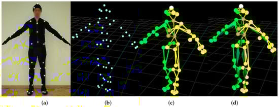
Figure 1. Stages of the motion capture pipeline: actor (a); registered markers (b); body mesh (c); mesh matched skeleton (d).

2.2. Functional Body Mesh

Functional body mesh (FBM) is a authors’ original contribution, that forms a framework for marker-wise mocap data processing, which incorporates also the kinematic structure of a represented object. The FBM structure is not given in advance, but it can be inferred based on the articulated object representative motions [11]. For human actors it resembles standard meshes, but it can be applied for virtually any vertebrates. It assumes the body is divided into rigid segments (submeshes), which are organized into a tree structure. The model represents the hierarchy of subjects’ kinematic structure, reflecting bonds between body segments, where every segment is a local rigid body model—usually based on an underlying bone.

The rigid segments maintain the distance between the markers and, additionally, for each child segment, one representative marker is assumed within the parent one, which is also assumed to maintain a constant distance from the child markers. The typical FBM for the human actor is shown in Figure 2b as a tree. The segments and constituent markers are located in nodes, whereas the parent marker is denoted on the parent–child edge.

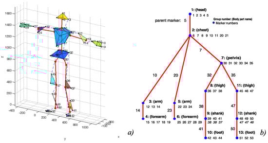
Figure 2. Outline of the body model (a), and corresponding parts hierarchy annotated with parents and siblings (b).

2.3. Previous Works

Gap filling is a classical problem frequently addressed in research on mocap technologies. It was in numerous works, which proposed various approaches. The existing methods can be divided into three main groups—skeleton-based, marker-wise, and coordinate-based.

A classical skeleton-based method was proposed by Herda et al. [12], they estimate skeleton motion and regenerate markers on the body envelope. Aristidou and Lanesby [13] proposed the other method based on a similar concept, where the skeleton is a source for constraints in inverse kinematics estimation of marker location. Also, Perepichka et al. [14] combined IK of skeleton model with deep NN to detect erroneously located markers and to place them on a probable trajectory. All aforementioned approaches require either to have a predefined skeleton or to infer the skeleton as the entry step of an algorithm.

The skeleton-free methods consider information from markers only, usually acknowledging the whole sequence as a single multivariable (matrix), thus losing the kinematic structure of the represented actor. They rely on various concepts, starting from the simple interpolating methods [15,16,17]. The proposal by Liu and McMillan [18] employed ‘local’ (neighboring markers) low-dimensional least squares models combined with PCA for missing marker reconstruction. A significant group of gap reconstruction proposals is based on the low-rank matrix completion methods. They employ various mathematical tools (e.g., matrix factorization with SVD) for the missing data completion, relying on inter marker correlations. Among the others, these methods are described in the following works [19,20]. Another approach is somewhat related: it is a fusion of several regressions and interpolation methods, which was proposed in [21].

Predicting markers (or joint) position is another concept that is the basis of gap-filling techniques. One such concept is a predictive model by Piazza et al. [22], which decomposes the motion into linear and circular and finds momentary predictors by curve fitting. More sophisticated dynamical models based on the Kalman filter (KF) are commonly applied. Wy and Boulanger [23] proposed a KF with velocity constraints; however, this achieved moderate success due to drift. A KF with an expectation-maximization algorithm was also used in two related approaches by Li et al.—DynaMMo [24], and BoLeRO [25] (the latter is actually Dynammo with bone length constraints). Another approach was proposed by Burke and Lanesby [26], who applied dimensionality reduction by PCA and then Kalman smoothing for the reconstruction of missing markers.

Another group of methods is dictionary-based. These algorithms recover the trajectories using a dictionary created from previously recorded sequences. They result in satisfactory outcomes as long the specific motion is in the database. They are represented by the works of Wang et al. [27], Aristidou et al. [28], and Zhang and van de Panne [29].

Finally, neural networks are another group of methods used in marker trajectory reconstruction. The task can be described as a sequence-to-sequence regression problem, whereas NN applied for regression has been recognized since the early 1990s in the work of Hornik [30]; hence, NN seems to be a natural choice for the task. Surprisingly, however, they become popular quite late. In the work of Fragkiadaki et al. [31], an encoder–recurrent-decoder (ERD) was proposed, employing long-short term memory (LSTM) as a recurrent layer. A similar approach (ERD) was proposed by Harvey et al. [32] for in-between motion generation on the basis of asmall amount of keyframes. Mall et al. [33] modified the ERD and proposed an encoder–bidirectional-filter (EBF) based on the bidirectional LSTM (BILSTM). In the work of Kucharenko et al. [34], a classical two-layer LSTM and window-based feed-forward NN (FFNN) were employed. A variant of ResNet is applied by Holden [35] to reconstruct marker positions from noisy data as a ttrajectory reconstruction task. A set of extensions to the plain LSTM were proposed by Ji et al. [36]; they introduced attention (a weighting mechanism) and LS-derived spatial constraints, which result in an improvement in performance. Convolution auto-encoders was proposed by Kaufmann et al. [37].

3. Materials and Methods

3.1. Proposed Regression Approach

The proposed approach involves employing various neural networks architectures for the regression task. These are FFNN and three variants of contemporary recursive neural networks—gated recurrent unit (GRU), long-short-term memory (LSTM), and bidirectional LSTM (BILSTM). In our proposal, these methods predict trajectories of lost markers on the basis of a local dataset—the trajectories of neighboring markers.

The proposed utilization procedure of NN differs from the scenario that is typically employed in machine learning. We do not feed the NNs with a massive amount of training sequences in advance to form a predictive model. Instead, we consider each sequence separately and try to reconstruct the gaps in individual motion trajectory on the basis of its own data only. This makes sense as long as the marker motion is correlated and most of the sequence is correct and representative enough. This is the same as for the other common regression methods, starting with the least squares. Therefore, the testing data are the whole ‘lost’ segment (gap), whereas the training is the remaining part of the trajectory. Depending on the gap sizes, and sequence length used in the experiment, the testing can be between 0.6% (for short gaps and long sequences) and up to 57.1% (for long gaps in short sequences).

The selection of such a non-typical approach requires a justification. It is likely that training the NN models for prediction of marker position in a conventional way, using a massive dataset of mocap sequences, would be able to generalize enough to adjust to different body sizes and motions. However, it will be tightly coupled with the marker configuration, not to mention the other actors, such as animals. The other issue is obtaining such a large amount of data. Despite our direct access to the lab resources, this is still quite a cumbersome task, since we believe these might be not enough, especially as the resources available online from various other labs are hardly usable, since they employ different marker setups.

The forecasting of timeseries is a typical problem addressed by RNNs [38]. Usually, numerous training and testing sequences allow for a prediction of the future states of the modelled system (e.g., power consumption or remaining useful life of devices). A more similar situation, where RNNs are also applied, is forecasting the time series for problems lacking massive training data (e.g., COVID-19 [39]). An analysis of LSTM architectures for similar cases is presented in [40]. However, in these works, the forecast of future values is based on the past values. What makes our case a bit different is the fact that we usually have to predict the value in-the-middle, so the past and future values are available.

3.1.1. Feed Forward Neural Network

FFNN is the simplest neural network architecture. In this architecture, the information flows in one direction, as its structure forms an acyclic directed graph. The neurons are modeled in the nodes with activation functions (usually sigmoid) using the weighted sum of inputs. These networks are typically organized into layers, where the output from the previous layer becomes an input to a successive one. This architecture of networks is employed for regression and classification tasks, either alone or as final stages in a larger structures (such as modern deep NN). The architecture of the NN that we employed is shown in Figure 3. The basic equation (output) of a single—k-th artificial neuron is given as:

$$y_k\left(x\right)=f\left(\sum _j{w}_{jk}{x}_j+b\right),$$

(1)

where $x_j$ is j-th input, $w_{kj}$ is j-th input weight, b—a bias value, f—is transfer (activation) function. Transfer function depends on the layer purpose; these are typically a sigmoid for hidden layers, threshold, linear, or softmax for final layers (for regression and classification problems, respectively), or others.

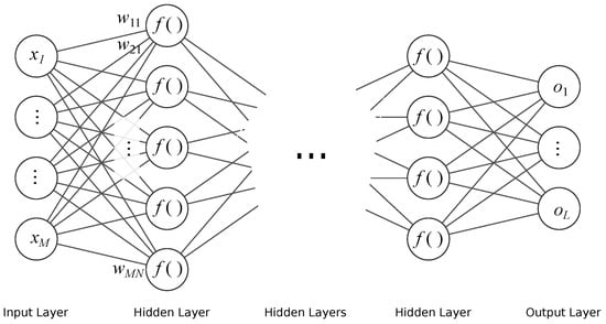
Figure 3. Schematic of FFNN.

3.1.2. Recurrent Neural Networks

Recurrent neural networks (RNN) are the types of architecture that employ cycles in NN structure; this allows for the consideration of current input value as well as preserving the previous inputs and internal states of NN in memory (and future ones for bidirectional architecture). Such an approach allows for NN to deal with timed processes and to recognize process dynamics, not just static values—it applies to such tasks as a signal prediction or recognition of sequences. Regarding the applicability, aside from classic problem dichotomy (classification and regression), RNN results might need another task differentiation. One must decide whether the task is a sequence-to-one or sequence-to-sequence problem, so the network has to return either a single result for the whole sequence or a single result for each data tuple in sequence. The prediction/regression task is a sequence-to-sequence problem, as demonstrated with RNNs in Figure 4 in different variants—both folded and unfolded, uni- and bi-directional.

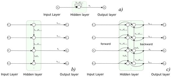
Figure 4. Usage of recurrent NNs in sequence to sequence task: (a) folded, (b) unfolded unidirectional variant, (c) unfolded bidirectional variant.

At present two types of neuron are predominantly applied in RNN–long short term memory (LSTM) and gated recurrent unit (GRU), of which the former is also applied in bidirectional variant (BILSTM). They evolved from a plain RNN called ‘vanilla’, and they prevent vanishing gradient problems when back-propagating errors in the learning process. Their detailed designs are unfolded in Figure 5. These cell types rely on the input information and information from previous time steps, and those previous states are represented in various ways. GRU passes an output (hidden signal h) between the steps, whereas LSTM also passes a h and internal cell state C. These values are interpreted as memory—h as short term, and C as long term. Their activation function is typical sigmoid, which is modeled with a hyperbolic tangent (tanh), but there are additional elements present in the cell. The contributing components, such as input or previous values, are subject to ‘gating’—their share is controlled by Hadamard product (element-wise product denoted as ⊙ or ⊗ in diagram) with 0–1 sigmoid function $\sigma \left(x\right)=\frac{1}{1+e^{-x}}$. The individual $\sigma$ values are obtained by weighted input and state values.

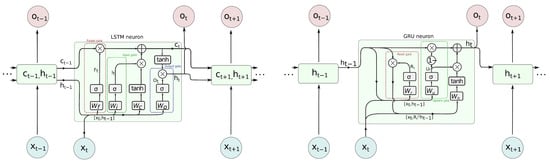
Figure 5. LSTM (left) and GRU (right) neurons in detail.

In more detail, in LSTM, we pass two variables $h,C$ and have three gates—forget, input and output. They govern how much of the respective contribution passes to further processing. The forget gate ($f_t$) decides how much of the past cell internal state ($C_{t-1}$) is to be kept; the input gate ($i_t$) controls how much new contribution ${\tilde{C}}_t$ caused by input ($x_t$) annd taken into the current cell state ($C_t$). Finally, the output gate ($o_t$) controls what part of activation is based on the cell internal state; ($C_t$) is taken as cell output ($h_t$). The equations are as follows:

$$\begin{array}{cc}\hfill f_t& =\sigma (W_f·[x_t,h_{t-1}]+b_f),\hfill \end{array}$$

(2)

$$\begin{array}{cc}\hfill i_t& =\sigma (W_i·[x_t,h_{t-1}]+b_f),\hfill \end{array}$$

(3)

$$\begin{array}{cc}\hfill {\tilde{C}}_t& =tanh(W_c·[x_t,h_{t-1}]+b_c),\hfill \end{array}$$

(4)

$$\begin{array}{cc}\hfill C_t& =f_t\odot C_{t-1}+i_t\odot {\tilde{C}}_t,\hfill \end{array}$$

(5)

$$\begin{array}{cc}\hfill o_t& =\sigma (W_o·[x_t,h_{t-1}]+b_f),\hfill \end{array}$$

(6)

$$\begin{array}{cc}\hfill h_t& =o_t\odot tanh\left(C_t\right).\hfill \end{array}$$

(7)

The detailed schematic of GRU is a bit simpler. Only one signal, hidden (layer output) value (h for hi), is passed between steps. There are two gates present—the reset gate ($r_t$), which controls how much past output ($h_{t-1}$) contributes to the overall cell activation, and the update gate ($u_t$), which controls how much current activation (${\tilde{h}}_t$) contributes to the final cell output.The above are described by the following equations:

$$\begin{array}{cc}\hfill u_t& =\sigma (W_u·[x_t,h_{t-1}]+b_u),\hfill \end{array}$$

(8)

$$\begin{array}{cc}\hfill r_t& =\sigma (W_u·[x_t,h_{t-1}]+b_u),\hfill \end{array}$$

(9)

$$\begin{array}{cc}\hfill {\tilde{h}}_t& =tanh(W_h·[x_t,r_t\odot h_{t-1}]+b_h),\hfill \end{array}$$

(10)

$$\begin{array}{cc}\hfill h_t& =(1-u_t)\odot h_{t-1}+u_t\odot {\tilde{h}}_t.\hfill \end{array}$$

(11)

3.1.3. Employed Reconstruction Methods

We compared the performance of five architectures of NN—two variants of FFNN and three RNN-FCs based on GRU, LSTM, and BILSTM; the outline of the latter is depicted in Figure 6. The detailed structures and hyperparameters of NNs were established empirically, since there are no strict rules or guidelines. Usually, this requires simulating, with parameters sweeping the domain of feasible numbers of layers and neurons [41]. We shared this approach and reviewed the performance of NN using the test data.

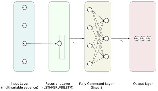
Figure 6. Proposed RNN-FC architecture for the regression task.

• FFNN${}_{\mathrm{lin}}$, with 1 hidden fully connected (FC) layer—containing 8 linear neurons;
• FFNN${}_{\tanh }$, with 1 hidden FC layer—containing 8 sigmoidal neurons;
• LSTM followed by 1 FC layer containing 8 sigmoidal neurons;
• GRU followed by 1 FC layer containing 8 sigmoidal neurons;
• BILSTM followed by 1 FC layer containing 8 sigmoidal neurons.

The output is three valued $x,y,z$ vectors, containing reconstructed marker coordinates.

3.1.4. Implementation Details

The training process was performed using 600 epochs, with the SGDM solver running on the GPU. It involved the whole input sequence with gaps excluded. There was a single instance of sequence in the batch. The sequence parts containing gaps were used as the test data; the remainder was used for training—therefore, the relative size of test part varies between 0.6% and 57.1%. The other parameters are:

• Initial Learn Rate: 0.01;
• Learn Rate Drop Factor: 0.9;
• Learn Rate Drop Period: 10;
• Gradient Threshold 0.7;
• Momentum: 0.8.

We also applied z-score normalization for the input and target data.

Additionally, for comparison, we used a pool of other methods, which should provide nice results for short-term gaps. These are interpolations: linear, spline, modified Akima (makima), piecewise cubic hermite interpolating polynomial (pchip), and the low-rank matrix completion method (mSVD0). All but linear interpolation methods are actually variants of piecewise Hermite cubic polynomial interpolations, which differ in the details of how they compute interpolant slopes. Spline is a generic method, whereas pchip tries to preserve shape, and makima avoids overshooting. However, mSVD [42] is an iterative method decomposing motion capture data with SVD and neglecting the least significant part of the basis transformed signal, reconstructing the original data with replacing missing values using reconstructed ones. The procedure finishes when convergence is reached. We implemented the algorithm, as outlined in [24].

The implementation of methods and experiments was carried out in Matlab 2021a using its implementations of numerical methods and deep learning toolbox.

3.2. Input Data Preparation

Constructing the predictor for certain markers, we obtained the locations from all the sibling markers and a single parent one, as they are organized within an FBM structure. For j-th marker ($X_j=[x_j,y_j,z_j]$), we consider parent ($X_p$) and sibling markers ($X_{s1},\dots ,X_{sL}$). To form an input vector, we take two of their values—one for the current moment and with one sample lag. The other variants with more lags or values raised to the higher powers were considered, but after preliminary tests, we neglected them since they did not improve performance.

Each input vector T, for the moment n, is quite long and is assembled of certain parts, as given below:

$$\begin{array}{cc}\hfill & T(n,\ast )=\left[\begin{array}{c}\stackrel{\mathrm{current}\mathrm{and}\mathrm{former}\mathrm{values}\mathrm{of}\mathrm{parent}\mathrm{marker} \left(p\right)}{\overbrace{x_p\left(n\right),y_p\left(n\right),z_p\left(n\right),x_p(n-1),y_p(n-1),z_p(n-1)}},\\ \stackrel{\mathrm{current}\mathrm{and}\mathrm{former}\mathrm{value}\mathrm{of}\mathrm{first}\mathrm{sibling}{s}_1}{\overbrace{x_{s1}\left(n\right),y_{s1}\left(n\right),z_{s1}\left(n\right),x_{s1}(n-1),y_{s1}(n-1),z_{s1}(n-1)}},\\ ⋮\\ \underset{\mathrm{current}\mathrm{and}\mathrm{former}\mathrm{value}\mathrm{of}\mathrm{last}\mathrm{sibling}{s}_L}{\underbrace{x_{sL}\left(n\right),y_{sL}\left(n\right),z_{sL}\left(n\right),x_{sL}(n-1),y_{sL}(n-1),z_{sL}(n-1)}}\end{array}\right].\hfill \end{array}$$

(12)

Finally, the input and output data are z-score standardized—zero centered and standard deviation scaled to 1, since such a step notably improves the final results.

3.3. Test Dataset

For testing purposes, we used a dataset (Table 1) acquired for professional purposes in the motion-capture laboratory. The ground truth sequences were obtained at the PJAIT human motion laboratory using the industrial-grade Vicon MX system. The system capture volume was 9 m × 5 m × 3 m. To minimize the impact of external interference such as infrared interference from sunlight or vibrations, all windows were permanently darkened and cameras were mounted on scaffolding instead of tripods. The system was equipped with 30 NIR cameras manufactured by Vicon: MX-T40, Bonita10, Vantage V5—wth 10 pieces of each kind.

Table 1. List of mocap sequence scenarios used for the testing.

No.	Name	Scenario	Duration	Difficulty
1	Static	Actor stands in the middle of scene, looking around and shifting from one foot to another, freely swinging arms	32 s	varied motions
2	Walking	Actor stands still at the edge of the scene, then walks straight for 6 m, then stands still	7 s	low dynamics, easy
3	Running	Actor stands in the middle of scene, then goes backwards to the edge of the scene and runs for 6 m, then goes backwards to the middle of the scene	16 s	moderate dynamics
4	Sitting	Actor stands in the middle of scene, then sits on a stool, and, after a few seconds, stands again	15 s	occlusions
5	Boxing	Actor stands in the middle of scene, and performs some fast boxing punches	14 s	high dynamics
6	Falling	Actor stands on 0.5 m elevation in the middle of scene, the walks to edge of platform, then falls on the mattress, lies for 2 s and stands	16 s	high dynamics, occlusions

During the recording, we employed a standard animation pipeline, where data were obtained with Vicon Blade software using a 53-marker setup. The trajectories were acquired at 100 Hz and, by default, they were processed in a standard, industrial-quality way, which includes manual data reviewing, cleaning and denoising, so they can be considered distortion-free.

Several parameters for the test sequences are also presented in Table 2. We selected these parameters as one could consider them to potentially describe prediction difficulty. They are various, and based on different concepts such as information theory, statistics, kinematics, and dynamics, but all characterize the variability in the Mocap signal. They are usually the average value per marker, except for standard deviation (std dev), which reports value per coordinate.

Table 2. Input sequence characteristics.

No	Entropy ($\mathit{H}\left(\mathit{X}\right)$)	Stddev (${\mathit{\sigma }}_{\mathit{X}}$)	Velocity ($\frac{\mathit{\partial }\mathit{X}}{\mathit{\partial }\mathit{t}}$)	Acc. ($\frac{{\mathit{\partial }}^2\mathit{X}}{\mathit{\partial }{\mathit{t}}^2}$)	Jerk ($\frac{{\mathit{\partial }}^3\mathit{X}}{\mathit{\partial }{\mathit{t}}^3}$)	Monotonicity	Complexity
	[Bits/Mark.]	[mm/Coordinate]	[m/s/Mark.]	$[\mathbf{m}/{\mathbf{s}}^2/\mathbf{Mark}.]$	$[\mathbf{m}/{\mathbf{s}}^3/\mathbf{Mark}.]$	[-]	[-]
1	12.697	129.705	0.208	1.561	64.817	0.352	0.027
2	13.943	941.123	0.773	6.476	829.271	0.582	0.000
3	15.710	982.342	0.895	6.176	643.337	0.379	0.001
4	10.231	135.356	0.190	2.863	452.142	0.347	0.016
5	11.356	121.094	0.259	3.557	507.975	0.323	0.023
6	14.152	601.140	0.589	6.703	799.039	0.745	0.007

Two non-obvious measures are enumerated: monotonicity and complexity. The monotonicity indicates, on average, the extent to which the coordinate is monotonic. For this purpose, we employed an average Spearman rank correlation, which can be described as follows:

$$monotonicity=\frac{1}{M}\sum _{m=1}^M\mathrm{corr}(\mathrm{rank}\left(X_i\right),1\dots N),$$

(13)

where $X_m$ is mth coordinate, M is number of coordinates, N is sequence length.

Complexity, on the other hand, is how we estimate the variability of poses in the sequence. For that purpose, we employed PCA, which identifies eigenposes as a new basis for the sequence. The corresponding eigenvalues describe how much of the overall variance is described by each of the eigenposes. Therefore, we decided to take the remainder of the fraction of variance described by the sum of the five largest eigenvalues (${\lambda }_i$) as a term describing how complex (or rather simple) the sequence is—the simpler the sequence, the more variance is described, with a few eigenposes. Therefore, our complexity measure is simply given as:

$$complexity=1-\sum _{i=1}^5{\lambda }_i/\sum _{i=1}^M{\lambda }_i,$$

(14)

where M is a number of coordinates.

3.4. Quality Evaluation

The natural criterion for the reconstruction task is root mean square error (RMSE), which, in our case, is calculated only for the time and marker, where the gaps occur:

$$\mathrm{RMSE}=\sqrt{\frac{1}{\left|W\right|}\sum _{i\in W}{({\widehat{X}}_i-X_i)}^2},$$

(15)

where W is a gap map, logically indexing locations of gaps, $\widehat{X}$ is a reconstructed coordinate, X is the original coordinate.

Additionally, we calculated RMSEs for individual gaps. Local RMSE is a variant of the above formula, and simply given as:

$$RMS{E}_k=\sqrt{\frac{1}{|w_k|}\sum _{i\in w_k}{({\widehat{X}}_i-X_i)}^2},$$

(16)

where $w_k\subset W$ is a single gap map logically indexing the location of k-th gap, $\widehat{X}$ is reconstructed coordinate, X is original coordinate. $RMS{E}_k$ is intended to reveal variability in reconstruction capabilities; hence, we used it to obtain statistical descriptors—mean, median, mode, and quartiles and interquartile range.

A more complex evaluation of regression models can be based on infromation criteria. These quality measures incorporate squared error and a number of tunable parameters, as they were designed by searching for a tradeoff between the number of tunable parameters and the obtained error. The two most popular ones are Bayesian Information Criterion (BIC) and Akaike Information Criterion (AIC). BIC is calculated as:

$$\mathrm{BIC}=nlog\left(MSE\right)+plog\left(n\right),$$

(17)

whereas AIC formula is as follows:

$$\mathrm{AIC}=nlog\left(MSE\right)+2p,$$

(18)

where: mean squared error $\mathrm{MSE}={\mathrm{RMSE}}^2$, n is a number of testing data, p is a number of tunable parameters.

3.5. Experimental Protocol

During the experiments, we simulated gap occurrence in perfectly reconstructed source sequences. We simulated gaps of different average lengths—10, 20, 50, 100 and 200 samples (0.1, 0.2, 0.5, 1, and 2 s, respectively). The assumed gap sizes were chosen to represent situations of various levels of difficulty, from short-and-simple to difficult ones, when gaps are long. For every gap length, we performed 100 simulation iterations, where the training and testing data do not intermix between simulation runs. The steps performed in every iteration are as follows:

• We introduce two gaps of assumed length (on average) to the random markers at random moments; actual values are stored as testing data;
• The model is trained using the remaining part of the sequence (all but gaps);
• We reconstruct (predict) the gaps using the pool of methods;
• The resulting values are stored for evaluation.

We report the results as RMSE and descriptive statistical descriptors for $RMS{E}_k$ for every considered reconstruction technique. Additionally, we verified the correlation between RMSE and the variability descriptors for sequences. It is intended to reveal what are the sources of difficulties in predicting the marker trajectories.

Gap Generation Procedure

The procedure of gap contamination, which was employed, introduces distortions into the sequences in a controlled way. The parameter characterizing the experiment is an average-length number of occurrences of gaps. the sequence of operations distorting the signal is as follows: at first, we draw moments to contaminate, then select a random marker. The duration of distortions and intervals is a Poisson process, an average length of distortion set-up according to the considered gap length in the experiment, whereas the interval length results from the sequence length and number of intervals, which, for two gaps per sequence, are three—ahead of the first gap, in-between, and after the second gap.

4. Results and Discussion

The section comprises two parts. First, we present RMSE results; they illustrate the performance of each of the considered gap reconstruction methods. The second part is the interpretation of results, searching for the aspects of Mocap sequence that might affect the resulting performance.

4.1. Gap Reconstruction Efficiency

The detailed numerical values are presented in Table 3 for the first sequence as an example. In the table, we also emphasize the best result for each measurement of gap size. Forclarity, the numerical outcomes of the experiment are only presented in this chapter with representative examples. To see the complete set of results in the tabular form, please refer to Appendix A. The complete results for the gap reconstruction are also demonstrated in a visual form in Figure 7. Additionally, the zoomed variant of the fragments of the plot (dash square annotated) for gaps 10–50 are presented in Figure 8.

Table 3. Quality measures for the static (No. 1) sequence.

Len		FFNN${}_{\mathbf{lin}}$	FFNN${}_{\mathbf{tanh}}$	LSTM	GRU	BILSTM	LIN	SPLINE	MAKIMA	PCHIP	mSVD
10	RMSE	3.830	5.375	2.410	2.494	1.801	1.267	0.348	0.610	0.737	1.267
	mean (${\mathrm{RMSE}}_k$)	3.280	4.869	2.175	2.290	1.708	0.971	0.243	0.468	0.512	0.971
	median (${\mathrm{RMSE}}_k$)	2.746	4.399	2.035	2.120	1.614	0.893	0.205	0.406	0.391	0.893
	mode (${\mathrm{RMSE}}_k$)	0.993	1.821	0.626	0.861	0.455	0.099	0.000	0.045	0.036	0.099
	stddev (${\mathrm{RMSE}}_k$)	1.893	2.209	0.939	0.989	0.573	0.695	0.216	0.336	0.458	0.695
	iqr (${\mathrm{RMSE}}_k$)	2.123	2.905	0.881	0.901	0.684	0.692	0.235	0.370	0.434	0.692
20	RMSE	3.474	5.114	2.559	2.527	2.082	3.366	1.191	1.914	2.354	3.366
	mean (${\mathrm{RMSE}}_k$)	3.187	4.775	2.371	2.351	1.903	2.694	0.933	1.525	1.738	2.694
	median (${\mathrm{RMSE}}_k$)	2.828	4.709	2.274	2.235	1.779	2.147	0.764	1.251	1.287	2.147
	mode (${\mathrm{RMSE}}_k$)	0.605	0.584	0.540	0.381	0.415	0.052	0.005	0.026	0.023	0.052
	stddev (${\mathrm{RMSE}}_k$)	1.442	1.871	0.891	0.898	0.826	1.831	0.664	1.045	1.483	1.831
	iqr (${\mathrm{RMSE}}_k$)	1.841	2.394	1.103	1.013	0.813	1.983	0.866	1.173	1.437	1.983
50	RMSE	3.813	5.910	5.001	4.041	4.777	10.363	5.517	6.928	7.677	10.363
	mean (${\mathrm{RMSE}}_k$)	3.401	5.434	4.233	3.445	3.958	9.207	4.572	6.027	6.573	9.207
	median (${\mathrm{RMSE}}_k$)	2.906	5.154	3.776	3.118	3.496	8.733	3.888	5.512	5.733	8.733
	mode (${\mathrm{RMSE}}_k$)	1.326	1.393	0.831	1.066	1.000	1.169	0.400	0.800	0.793	1.169
	stddev (${\mathrm{RMSE}}_k$)	1.688	2.168	2.430	1.921	2.448	4.464	2.852	3.174	3.764	4.464
	iqr (${\mathrm{RMSE}}_k$)	1.421	2.216	2.169	1.642	2.282	6.078	2.418	3.770	4.373	6.078
100	RMSE	4.759	7.805	10.798	7.678	10.716	24.634	12.548	15.231	18.746	24.634
	mean (${\mathrm{RMSE}}_k$)	4.233	7.134	9.460	6.721	9.302	21.812	11.236	13.587	16.108	21.812
	median (${\mathrm{RMSE}}_k$)	3.658	6.329	8.333	5.953	8.198	21.129	10.345	12.875	14.785	21.129
	mode (${\mathrm{RMSE}}_k$)	1.517	2.252	1.377	1.465	1.400	3.266	2.546	1.986	1.937	3.266
	stddev (${\mathrm{RMSE}}_k$)	2.132	3.143	5.114	3.692	5.230	11.305	5.472	6.825	9.556	11.305
	iqr (${\mathrm{RMSE}}_k$)	2.215	3.473	5.650	4.217	5.700	14.536	6.850	8.029	11.019	14.536
200	RMSE	9.959	18.970	33.147	27.987	33.104	62.786	34.481	47.259	56.570	62.786
	mean (${\mathrm{RMSE}}_k$)	9.062	17.303	30.204	24.837	30.135	55.099	31.616	41.676	48.789	55.099
	median (${\mathrm{RMSE}}_k$)	8.683	16.200	28.352	22.655	28.462	49.641	29.914	38.410	42.155	49.641
	mode (${\mathrm{RMSE}}_k$)	2.404	3.973	5.523	4.263	5.010	8.510	6.518	6.459	6.033	8.510
	stddev (${\mathrm{RMSE}}_k$)	4.013	7.631	13.450	12.743	13.503	29.934	13.511	22.022	28.463	29.934
	iqr (${\mathrm{RMSE}}_k$)	5.084	9.413	18.231	16.895	18.436	48.864	17.125	36.315	46.222	48.864

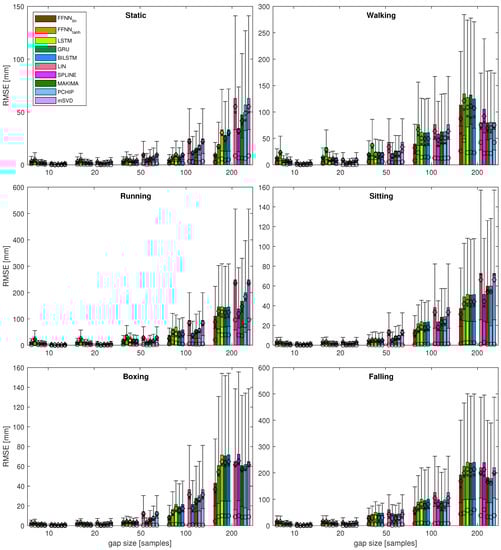
Figure 7. Results for most of the quality measures for all the test sequences. Bars denote $RMSE$; for $RMS{E}_k$: ⋄ denotes mean value, × denotes median, ∘ denotes mode, whiskers indicate IQR; standard deviation is not depicted here; dash-outlined areas are zoomed in Figure 8.

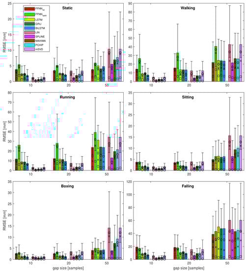
Figure 8. Results of the most of the quality measures for all the test sequences—zoomed variant for gaps 10, 20, and 50. Bars denote $RMSE$; for $RMS{E}_k$: ⋄ denotes mean value, × denotes median, ∘ denotes mode, whiskers indicate IQR; standard deviation is not depicted here.

The first observation, regarding the performance measures, is the fact that the results are very coherent, regardless of which measure was used. This is shown in Figure 7, where all the symbols coherently denote statistical descriptors scale. It is also clearly visible in the values emphasized in Table 3, where all measures but one (mode) indicate the same best (smallest) results. Hence, we can use a single quality measure; in our case, we assumed RMSE for further analysis.

Analyzing the results for several sequences, various observations regarding the performance of the considered methods can be noted. These are listed below:

• It can be seen that, for the short gaps, interpolation methods outperform any of the NN-based methods.
• For gaps that are 50 samples long, the results become less obvious and NN results are no worse or (usually) better than interpolation methods.
• Linear FFNN usually performed better than any other methods (including non-linear FFNN${}_{\tanh }$), for gaps of 50 samples or longer, for most of the sequences.
• In very rare cases of short-gap cases, RNNs performed better than FFNN${}_{\mathrm{lin}}$, but, in general, simpler FFNN${}_{\mathrm{lin}}$ outperformed more complex NN models.
• There are two situations when the FFNN${}_{\mathrm{lin}}$, performed no better or worse than interpolation methods (walking and falling). This occurred for sequences with larger monotonicity values in Table 2. They have also increased velocity/acceleration/jerk values; the ‘running’ sequence has similar values for these, but FFNN${}_{\mathrm{lin}}$ perform the best in this case, so the kinematic/dynamic parameters should not be considered.

Looking at the results of various NN architectures, it might be surprising that the sophisticated RNNs often returned worse results than relatively simple FFNN, especially for relatively long gaps. Conversely, one might expect that RNNs would outperform other methods, since they would be able to model longer-term dependencies in the motion. Presumably, the source of such a result is in the limited amount of training data, which, depending on the length of the source file, varies between hundreds and thousands of registered coordinates. Therefore, solvers are unable to find actually good values for a massive amount of parameters—see Table 4 for the formulas and numbers of learnable parameters for an exemplary case when input comprises 30 values—coordinates of four siblings and a parent at current and previous frames.

Table 4. List of mocap sequence scenarios used for the testing.

NN Type	Number of Learnable Parameters	Value for Exemplary Case
FFNN:	$hiddenLayerSize\times inputvectorSize+hiddenLayerSize$	275
	$+3\times hiddenLayerSize+3$
LSTM:	$4\times hiddenRecurrentNeurons\times inputvectorSize$	22,023
	$+4\times hiddenRecurrentNeurons\times hiddenRecurrentNeurons$
	$+4\times hiddenRecurrentNeurons$
	$+3\times hiddenRecurrentNeurons+3$
GRU:	$3\times hiddenRecurrentNeurons\times inputvectorSize$	16,563
	$+3\times hiddenRecurrentNeurons\times hiddenRecurrentNeurons$
	$+3\times hiddenRecurrentNeurons$
	$+3\times hiddenRecurrentNeurons+3$
BILSTM:	$8\times hiddenRecurrentNeurons\times inputvectorSize$	47,043
	$+8\times hiddenRecurrentNeurons\times hiddenRecurrentNeurons$
	$+8\times hiddenRecurrentNeurons$
	$+3\times 2\times hiddenRecurrentNeurons+3$

An obvious solution to such an issue would be increasing the training data. We could achieve this by employing very long recordings or by using numerous recordings. In the former, it would be difficult to achieve long enough recordings; the latter is different from the case which we try to address, where we only obtain a fresh mocap recording and reconstruct it with the minimal model given by FBM. Training the predictive model in advance with a massive amount of data is, of course, an interesting solution, but would cost the generality. For every marker configuration, a separate set of predicting NNs would need to be trained, so the result would only be practical for standardized body models.

Considering the length of the training sequences, its contribution to the final results seems far less important than other factors, at least within the range of considered cases. The analysis of its influence is illustrated in Figure 9. Since the MSE results are entangled, we employed two additional information criterions, Akaike Information Criterion (AIC), Bayesian Information Criterion (BIC), which disentangle the results by accounting for the number of trainable parameters. For every sequence and every NN model, we obtain a series of five results, which decrease, as the training sequence grows longer when we have shorter gaps (i.e., the annotated quintuple in the Figure). Analyzing the results in Figure 9, it is most convenient to observe this in the AIC/BIC plots since, for each model, the number of parameters remains the same (Table 4), so we can easily compare the results of the testing sequences. The zoomed versions (to the right) reveal differences at appropriate scales for the RNN results.

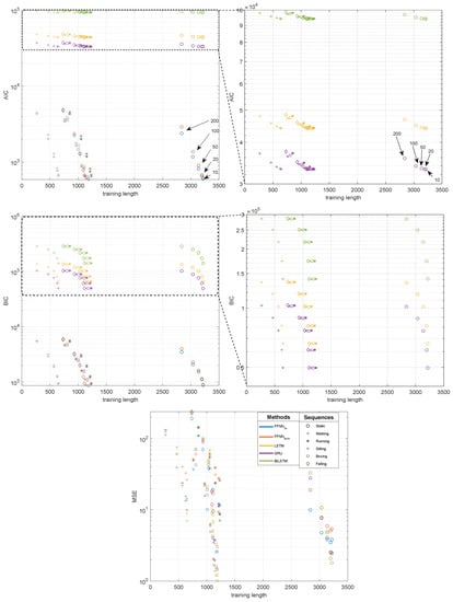
Figure 9. Influence of training sequence length on the quality of obtained results for NN methods: Akaike Information Criterion (AIC), Bayesian Information Criterion (BIC) and MSE.

Lookng at the reults, we observe that, regardless the length of the training sequence, the MSE (AIC/BIC) of the NN model remains at the same order of magnitude—this is clearly visible in the Figure, where we have very similar values for each gap size for variable sequences (represented as different marker shapes) for each of the NN types (represented by a color). The most notable reduction in the error is probably observed with the increased sequence length, when the sequence (Seq. 1—static) is several folds longer than the others. However, we cannot observe this difference for shorter sequences in our data, with notably different lengths (e.g., walking—running). The quality of prediction could be likely improved if the recordings were longer, but, in everyday praxis, the length of the motion caputre sequences is only minutes, so one should not expect the results for RNN data to be notably improved compared to those for FFNN.

The observations hold for both FFNN models and all RNNs. These ambiguous outcomes confirm the results shown in [40], where the quality of results does not depend on the length of the training data in a straightforward way.

4.2. Motion Factors Affecting Performance

In this section, we try to identify the correlation in which features (parameters) of the input sequences relate to the performance of gap-filling methods. The results presented here are concise; we only present and discuss the most conclusive results. The complete tables containing correlation values for all gap sizes are presented in Appendix B.

Foremost, a generalized view into the correlation between gap-filling outcomes and input sequence characteristics is given in Table 5. It contains Pearson correlation coefficients (CC) between RMSE and input sequence characteristic parameters; the values are Pearson CCs, averaged across all the considered gap sizes. Additionally, for the interpretation of the results, in Table 6, we provide CCs between RMSE and the descriptive parameters for the whole sequences for all the test recordings.

Table 5. Correlation between RMSE and sequence parameters (averaged for all gap sizes).

	FFNN${}_{\mathbf{lin}}$	FFNN${}_{\mathbf{tanh}}$	LSTM	GRU	BILSTM	LIN	SPLINE	MAKIMA	PCHIP	mSVD
Entropy	0.708	0.793	0.775	0.736	0.735	0.680	0.486	0.624	0.630	0.680
Stddev	0.741	0.892	0.805	0.781	0.778	0.706	0.517	0.653	0.631	0.706
Velocity	0.744	0.886	0.813	0.784	0.781	0.713	0.521	0.656	0.640	0.713
Acceleration	0.905	0.912	0.903	0.907	0.890	0.854	0.791	0.844	0.818	0.854
Jerk	0.803	0.794	0.777	0.799	0.779	0.753	0.758	0.763	0.725	0.753
Monotonicity	0.900	0.713	0.798	0.847	0.819	0.824	0.926	0.888	0.862	0.824
Complexity	−0.779	−0.886	−0.815	−0.804	−0.794	−0.742	−0.589	−0.702	−0.670	−0.742

Table 6. Correlation between sequence parameters.

	Entropy	Stddev	Velocity	Acceleration	Jerk	Monotonicity	Complexity
Entropy	1.000	0.869	0.898	0.730	0.459	0.465	−0.712
Stddev	0.869	1.000	0.992	0.879	0.732	0.501	−0.949
Velocity	0.898	0.992	1.000	0.890	0.731	0.477	−0.929
Acceleration	0.730	0.879	0.890	1.000	0.941	0.735	−0.913
Jerk	0.459	0.732	0.731	0.941	1.000	0.695	−0.847
Monotonicity	0.465	0.501	0.477	0.735	0.695	1.000	−0.560
Complexity	−0.712	−0.949	−0.929	−0.913	−0.847	−0.560	1.000
				p-values
Entropy	1.000	0.025	0.015	0.100	0.360	0.353	0.112
Stddev	0.025	1.000	0.000	0.021	0.098	0.311	0.004
Velocity	0.015	0.000	1.000	0.017	0.099	0.338	0.007
Acceleration	0.100	0.021	0.017	1.000	0.005	0.096	0.011
Jerk	0.360	0.098	0.099	0.005	1.000	0.125	0.033
Monotonicity	0.353	0.311	0.338	0.096	0.125	1.000	0.248
Complexity	0.112	0.004	0.007	0.011	0.033	0.248	1.000

Knowing that correlation, as a statistical measure, makes little sense for a sparse dataset, we treat it as a kind of measurement of co-linearity between the measures. However, for part of the parameters, the (high) correlation values are connected, with quite satisfactory low p-values; these are given in Appendix B.

Looking into the results in Table 5, we observe that all the considered sequence parameters are related, to some extent, to RMSE. However, for all the gap-filling methods, we identified two key parameters that have higher CCs than the others. These are acceleration and monotonicity, which seem to be promising candidate measures for describing the susceptibility of sequences to the employed reconstruction methods.

Regarding inter-parameter correlations in Table 6, we can observe that most of the measures are correlated with each other. This is expected, since kinematic/dynamic parameters are connected with the location of the markers over time, so values such as entropy, position standard deviation, velocity, acceleration, and jerk are correlated (for the derivatives, the smaller the difference in the derivative order, the higher the CCs).

On the other hand, the two less typical measures, monotonicity and complexity, are different; therefore, their correlation with the other measures is less predictable. Complexity appeared to have a notable negative correlation with most of the typical measures. Monotonicity, on the other hand, is more interesting. Since it is only moderately correlated with remaining measures, it still has quite a high CC, with RMSEs for all the gap reconstruction methods. Therefore, we can suppose this describes an aspect of the sequence that is independent of the other measures, which is related to susceptibility to the gap reconstruction procedures.

5. Summary

In this article, we addressed the issue of filling the gaps that occurred in the mocap signal. We considered this to be a regressive problem and reviewed the results of several NN-based regressors, which were compared with several interpolation and low-rank matrix completion (mSVD) methods.

Generally, in the case of short gaps, the interpolation methods returned the best results, but since the gaps became longer, part of the NNs gained an advantage. We reviewed five variants of neural networks. Surprisingly, the tests revealed that simple linear FFNNs, using momentary (current and previous sample) and local (from neighboring markers) coordinates as input data, outperformed quite advanced recurrent NNs for the longer gaps. For the shorter gaps, RNNs offered better results, but all the NNs were outperformed by interpolations. The boundary between ’long’ and ’short’ terms are gaps of 50 samples long. Finally, we were able to identify which factors of the input mocap sequence influence the reconstruction errors.

The approach to the NNs given here does not incorporate skeletal information. Instead, the kinematic structure is based on the FBM framework and all the predictions are performed with the local data, as obtained from FBM. Currently, none of the analyzed approaches considered body constraints such as limb length or size, but we can easily obtain such information from the FBM model. We plan to apply this as an additional processing stage in the future. In the future, we plan to test more sophisticated NN architectures, such as combined LSTM convolution, or averaged multiregressions.

References

- Kitagawa, M.; Windsor, B. MoCap for Artists: Workflow and Techniques for Motion Capture; Elsevier: Amsterdam, The Netherlands; Focal Press: Boston, MA, USA, 2008. [Google Scholar]
- Menache, A. Understanding Motion Capture for Computer Animation, 2nd ed.; Morgan Kaufmann: Burlington, MA, USA, 2011. [Google Scholar]
- Mündermann, L.; Corazza, S.; Andriacchi, T.P. The evolution of methods for the capture of human movement leading to markerless motion capture for biomechanical applications. J. Neuroeng. Rehabil. 2006, 3, 6. [Google Scholar] [CrossRef] [PubMed]
- Szczęsna, A.; Błaszczyszyn, M.; Pawlyta, M. Optical motion capture dataset of selected techniques in beginner and advanced Kyokushin karate athletes. Sci. Data 2021, 8, 13. [Google Scholar] [CrossRef] [PubMed]
- Świtoński, A.; Mucha, R.; Danowski, D.; Mucha, M.; Polański, A.; Cieślar, G.; Wojciechowski, K.; Sieroń, A. Diagnosis of the motion pathologies based on a reduced kinematical data of a gait. PrzegląD Elektrotechniczny 2011, 87, 173–176. [Google Scholar]
- Lachor, M.; Świtoński, A.; Boczarska-Jedynak, M.; Kwiek, S.; Wojciechowski, K.; Polański, A. The Analysis of Correlation between MOCAP-Based and UPDRS-Based Evaluation of Gait in Parkinson’s Disease Patients. In Brain Informatics and Health; Ślęzak, D., Tan, A.H., Peters, J.F., Schwabe, L., Eds.; Number 8609 in Lecture Notes in Computer Science; Springer International Publishing: Cham, Switzerland, 2014; pp. 335–344. [Google Scholar] [CrossRef]
- Josinski, H.; Świtoński, A.; Stawarz, M.; Mucha, R.; Wojciechowski, K. Evaluation of rehabilitation progress of patients with osteoarthritis of the hip, osteoarthritis of the spine or after stroke using gait indices. Przegląd Elektrotechniczny 2013, 89, 279–282. [Google Scholar]
- Windolf, M.; Götzen, N.; Morlock, M. Systematic accuracy and precision analysis of video motion capturing systems—Exemplified on the Vicon-460 system. J. Biomech. 2008, 41, 2776–2780. [Google Scholar] [CrossRef]
- Jensenius, A.; Nymoen, K.; Skogstad, S.; Voldsund, A. A Study of the Noise-Level in Two Infrared Marker-Based Motion Capture Systems. In Proceedings of the 9th Sound and Music Computing Conference, SMC 2012, Copenhagen, Denmark, 11–14 July 2012; pp. 258–263. [Google Scholar]
- Skurowski, P.; Pawlyta, M. On the Noise Complexity in an Optical Motion Capture Facility. Sensors 2019, 19, 4435. [Google Scholar] [CrossRef] [PubMed]
- Skurowski, P.; Pawlyta, M. Functional Body Mesh Representation, A Simplified Kinematic Model, Its Inference and Applications. Appl. Math. Inf. Sci. 2016, 10, 71–82. [Google Scholar] [CrossRef]
- Herda, L.; Fua, P.; Plankers, R.; Boulic, R.; Thalmann, D. Skeleton-based motion capture for robust reconstruction of human motion. In Proceedings of the Proceedings Computer Animation 2000, Philadelphia, PA, USA, 3–5 May 2000; pp. 77–83, ISSN: 1087-4844. [Google Scholar] [CrossRef]
- Aristidou, A.; Lasenby, J. Real-time marker prediction and CoR estimation in optical motion capture. Vis. Comput. 2013, 29, 7–26. [Google Scholar] [CrossRef]
- Perepichka, M.; Holden, D.; Mudur, S.P.; Popa, T. Robust Marker Trajectory Repair for MOCAP using Kinematic Reference. In Motion, Interaction and Games; Association for Computing Machinery: New York, NY, USA, 2019; MIG’19; pp. 1–10. [Google Scholar] [CrossRef]
- Lee, J.; Shin, S.Y. A hierarchical approach to interactive motion editing for human-like figures. In Proceedings of the 26th Annual Conference on Computer Graphics and Interactive Techniques, Los Angeles, CA, USA, 8–13 August 1999; ACM Press/Addison-Wesley Publishing Co.: New York, NY, USA, 1999; pp. 39–48. [Google Scholar] [CrossRef]
- Howarth, S.J.; Callaghan, J.P. Quantitative assessment of the accuracy for three interpolation techniques in kinematic analysis of human movement. Comput. Methods Biomech. Biomed. Eng. 2010, 13, 847–855. [Google Scholar] [CrossRef]
- Reda, H.E.A.; Benaoumeur, I.; Kamel, B.; Zoubir, A.F. MoCap systems and hand movement reconstruction using cubic spline. In Proceedings of the 2018 5th International Conference on Control, Decision and Information Technologies (CoDIT), Thessaloniki, Greece, 10–13 April 2018; pp. 1–5. [Google Scholar] [CrossRef]
- Liu, G.; McMillan, L. Estimation of missing markers in human motion capture. Vis. Comput. 2006, 22, 721–728. [Google Scholar] [CrossRef]
- Lai, R.Y.Q.; Yuen, P.C.; Lee, K.K.W. Motion Capture Data Completion and Denoising by Singular Value Thresholding. In Eurographics 2011—Short Papers; Avis, N., Lefebvre, S., Eds.; The Eurographics Association: Geneve, Switzerland, 2011. [Google Scholar] [CrossRef]
- Gløersen, Ø.; Federolf, P. Predicting Missing Marker Trajectories in Human Motion Data Using Marker Intercorrelations. PLoS ONE 2016, 11, e0152616. [Google Scholar] [CrossRef]
- Tits, M.; Tilmanne, J.; Dutoit, T. Robust and automatic motion-capture data recovery using soft skeleton constraints and model averaging. PLoS ONE 2018, 13, e0199744. [Google Scholar] [CrossRef]
- Piazza, T.; Lundström, J.; Kunz, A.; Fjeld, M. Predicting Missing Markers in Real-Time Optical Motion Capture. In Modelling the Physiological Human; Magnenat-Thalmann, N., Ed.; Number 5903 in Lecture Notes in Computer Science; Springer: Berlin/Heidelberg, Germany, 2009; pp. 125–136. [Google Scholar]
- Wu, Q.; Boulanger, P. Real-Time Estimation of Missing Markers for Reconstruction of Human Motion. In Proceedings of the 2011 XIII Symposium on Virtual Reality, Uberlandia, Brazil, 23–26 May 2011; pp. 161–168. [Google Scholar] [CrossRef]
- Li, L.; McCann, J.; Pollard, N.S.; Faloutsos, C. DynaMMo: Mining and summarization of coevolving sequences with missing values. In Proceedings of the 15th ACM SIGKDD International Conference on Knowledge Discovery and Data Mining; Association for Computing Machinery: New York, NY, USA, 2009; pp. 507–516. [Google Scholar] [CrossRef]
- Li, L.; McCann, J.; Pollard, N.; Faloutsos, C. BoLeRO: A Principled Technique for Including Bone Length Constraints in Motion Capture Occlusion Filling. In Proceedings of the 2010 ACM SIGGRAPH/Eurographics Symposium on Computer Animation; Eurographics Association: Aire-la-Ville, Switzerland, 2010; pp. 179–188. [Google Scholar]
- Burke, M.; Lasenby, J. Estimating missing marker positions using low dimensional Kalman smoothing. J. Biomech. 2016, 49, 1854–1858. [Google Scholar] [CrossRef]
- Wang, Z.; Liu, S.; Qian, R.; Jiang, T.; Yang, X.; Zhang, J.J. Human motion data refinement unitizing structural sparsity and spatial-temporal information. In Proceedings of the IEEE 13th International Conference on Signal Processing (ICSP), Chengdu, China, 6–10 November 2017; pp. 975–982. [Google Scholar]
- Aristidou, A.; Cohen-Or, D.; Hodgins, J.K.; Shamir, A. Self-similarity Analysis for Motion Capture Cleaning. Comput. Graph. Forum 2018, 37, 297–309. [Google Scholar] [CrossRef]
- Zhang, X.; van de Panne, M. Data-driven autocompletion for keyframe animation. In Proceedings of the 11th Annual International Conference on Motion, Interaction, and Games, New York, NY, USA, 8–10 November 2018; Association for Computing Machinery: New York, NY, USA, 2018; pp. 1–11. [Google Scholar] [CrossRef]
- Hornik, K. Approximation capabilities of multilayer feedforward networks. Neural Netw. 1991, 4, 251–257. [Google Scholar] [CrossRef]
- Fragkiadaki, K.; Levine, S.; Felsen, P.; Malik, J. Recurrent Network Models for Human Dynamics. In Proceedings of the 2015 IEEE International Conference on Computer Vision (ICCV), Santiago, Chile, 7–13 December 2015; pp. 4346–4354, ISSN: 2380-7504. [Google Scholar] [CrossRef]
- Harvey, F.G.; Yurick, M.; Nowrouzezahrai, D.; Pal, C. Robust motion in-betweening. ACM Trans. Graph. 2020, 39, 60:60:1–60:60:12. [Google Scholar] [CrossRef]
- Mall, U.; Lal, G.R.; Chaudhuri, S.; Chaudhuri, P. A Deep Recurrent Framework for Cleaning Motion Capture Data. arXiv 2017, arXiv:1712.03380. [Google Scholar]
- Kucherenko, T.; Beskow, J.; Kjellström, H. A Neural Network Approach to Missing Marker Reconstruction in Human Motion Capture. arXiv 2018, arXiv:1803.02665. [Google Scholar]
- Holden, D. Robust solving of optical motion capture data by denoising. ACM Trans. Graph. 2018, 37, 165:1–165:12. [Google Scholar] [CrossRef]
- Ji, L.; Liu, R.; Zhou, D.; Zhang, Q.; Wei, X. Missing Data Recovery for Human Mocap Data Based on A-LSTM and LS Constraint. In Proceedings of the 2020 IEEE 5th International Conference on Signal and Image Processing (ICSIP), Nanjing, China, 23–25 October 2020; pp. 729–734. [Google Scholar] [CrossRef]
- Kaufmann, M.; Aksan, E.; Song, J.; Pece, F.; Ziegler, R.; Hilliges, O. Convolutional Autoencoders for Human Motion Infilling. arXiv 2020, arXiv:2010.11531. [Google Scholar]
- Torres, J.F.; Hadjout, D.; Sebaa, A.; Martínez-Álvarez, F.; Troncoso, A. Deep Learning for Time Series Forecasting: A Survey. Big Data 2021, 9, 3–21. [Google Scholar] [CrossRef] [PubMed]
- Shahid, F.; Zameer, A.; Muneeb, M. Predictions for COVID-19 with deep learning models of LSTM, GRU and Bi-LSTM. Chaos Solitons Fractals 2020, 140, 110212. [Google Scholar] [CrossRef] [PubMed]
- Siami-Namini, S.; Tavakoli, N.; Namin, A.S. The Performance of LSTM and BiLSTM in Forecasting Time Series. In Proceedings of the 2019 IEEE International Conference on Big Data (Big Data), Los Angeles, CA, USA, 9–12 December 2019; pp. 3285–3292. [Google Scholar] [CrossRef]
- Czekalski, P.; Łyp, K. Neural network structure optimization in pattern recognition. Stud. Inform. 2014, 35, 17–32. [Google Scholar]
- Srebro, N.; Jaakkola, T. Weighted low-rank approximations. In Proceedings of the Twentieth International Conference on International Conference on Machine Learning, Washington, DC, USA, 21–24 August 2003; AAAI Press: Washington, DC, USA, 2003; pp. 720–727. [Google Scholar]
Publisher’s Note: MDPI stays neutral with regard to jurisdictional claims in published maps and institutional affiliations. |
© 2021 by the authors. Licensee MDPI, Basel, Switzerland. This article is an open access article distributed under the terms and conditions of the Creative Commons Attribution (CC BY) license (https://creativecommons.org/licenses/by/4.0/).