
On the Optimization of Regression-Based Spectral Reconstruction †


Abstract
:1. Introduction
2. Background
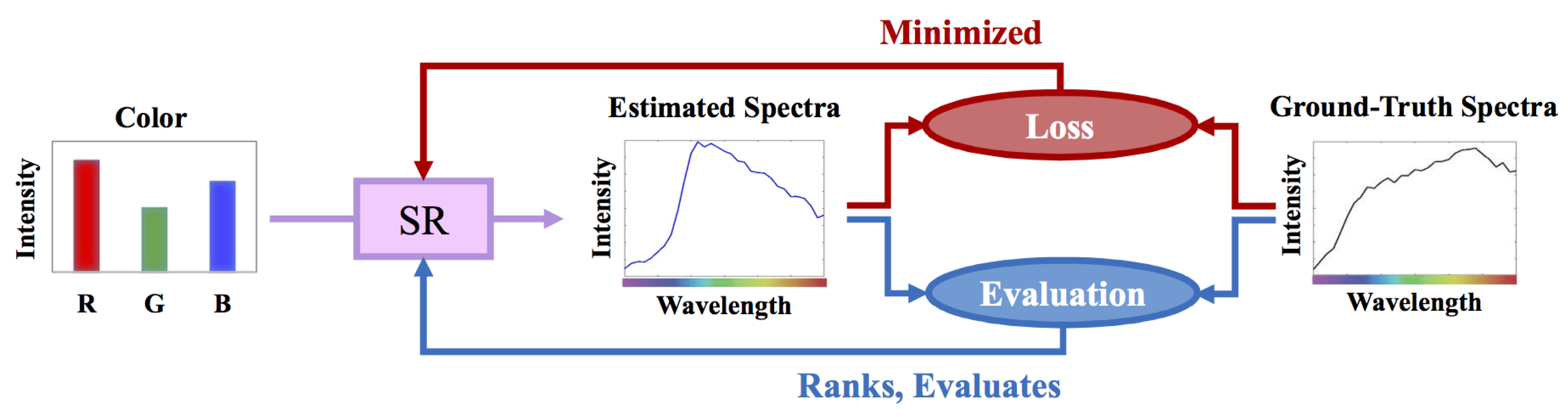
2.1. Regression-Based Spectral Reconstruction
2.1.1. Linear Regression
2.1.2. Nonlinear Regressions
2.1.3. A+ Sparse Coding
2.2. Least-Squares Minimization
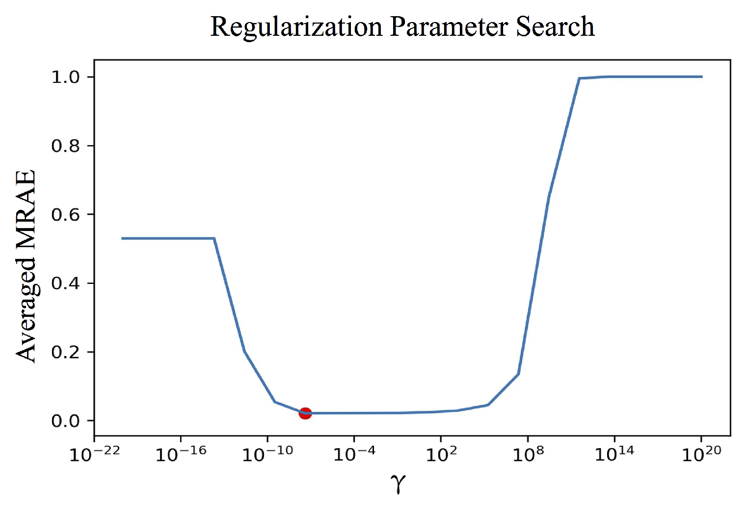
2.2.1. The Overfitting Problem and Regularized Least Squares
2.3. RMSE versus MRAE Error Measures
3. Rethinking the Optimization of Regression for Spectral Reconstruction
3.1. Per-Channel Regularization
3.2. Relative-Error Least Squares Minimization
3.3. Relative-Error Least Absolute Deviation Minimization
| Algorithm 1: Solving RELAD regression (Equation (24)) by IRLS algorithm. |
|
4. Experiment
4.1. The Regression Models
4.2. Preparing Ground-Truth Datasets
4.3. Training, Validation, and Testing
- Trial #1—Training: & , Validation: , Testing:
- Trial #2—Training: & , Validation: , Testing:
- Trial #3—Training: & , Validation: , Testing:
- Trial #4—Training: & , Validation: , Testing: .
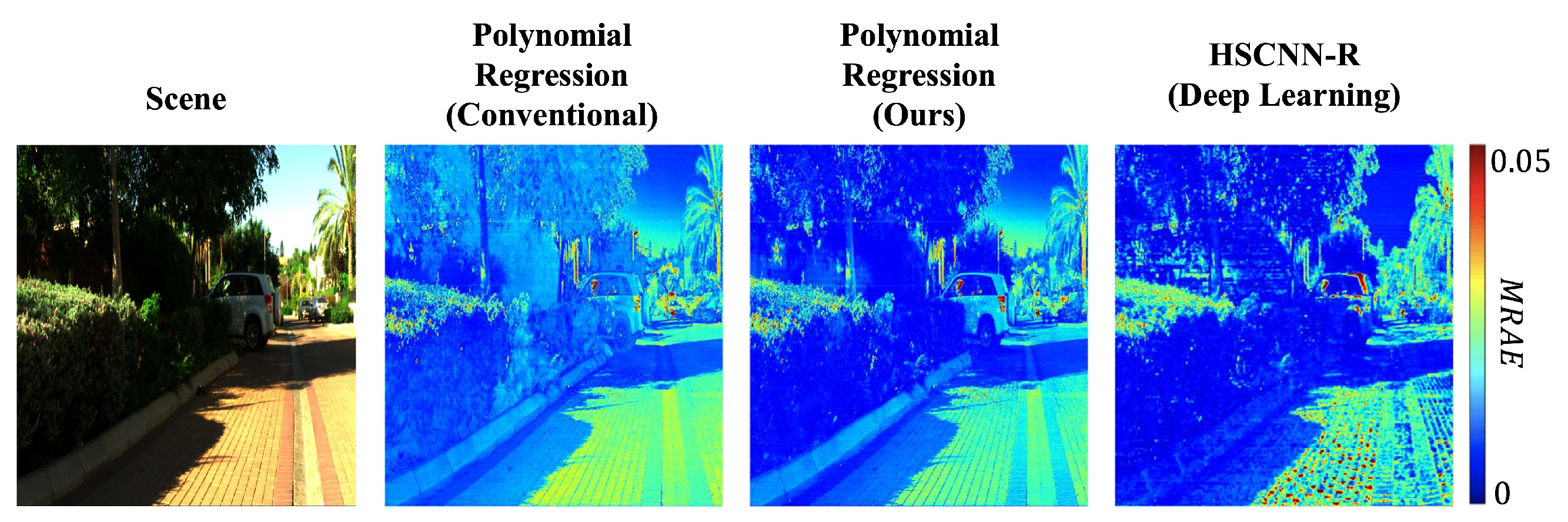
5. Results
5.1. Mean and Worst-Case Performance
5.2. Computational Time
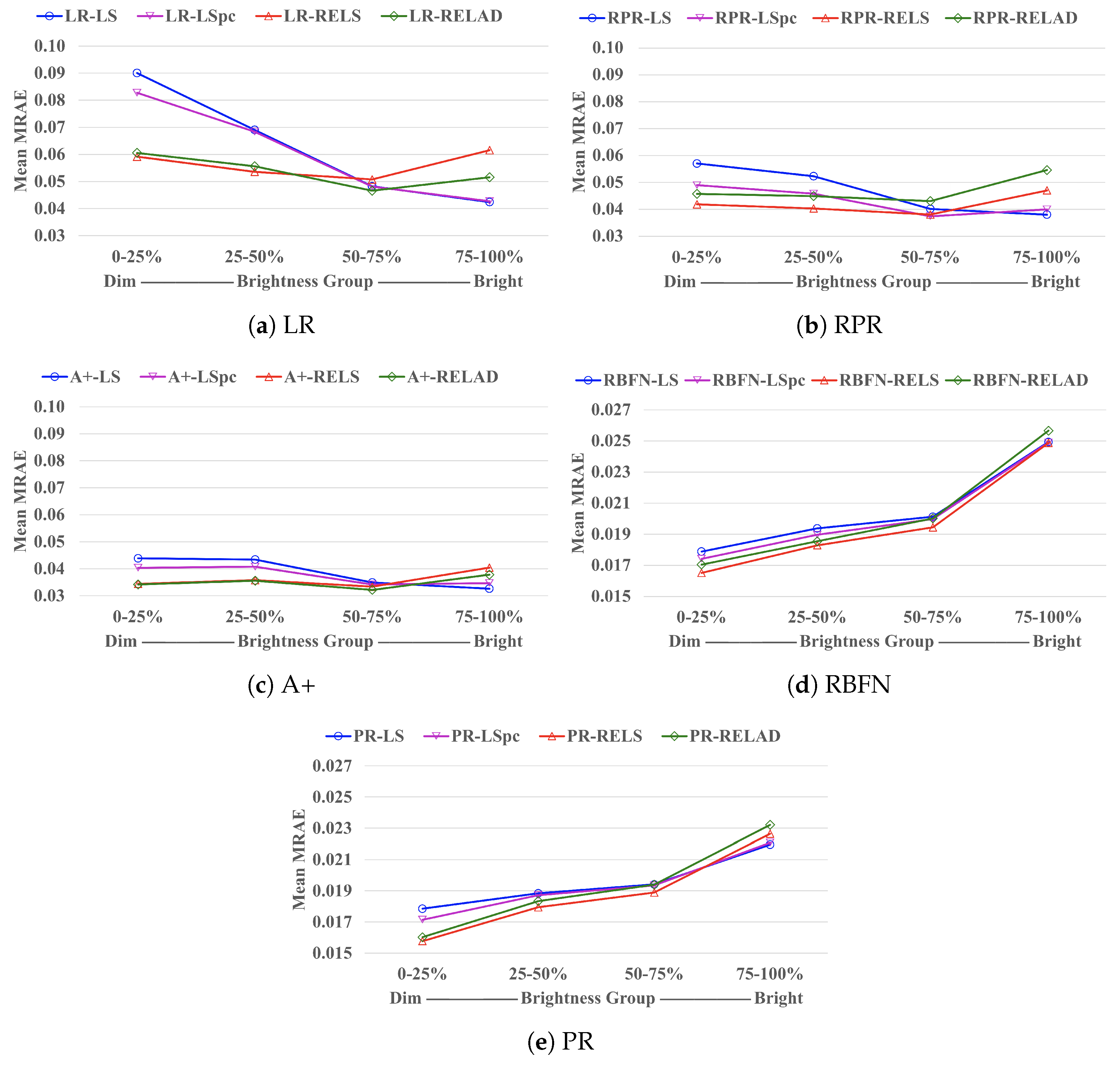
5.3. Brightness Dependence
6. Conclusions
Supplementary Materials
Author Contributions
Funding
Institutional Review Board Statement
Informed Consent Statement
Data Availability Statement
Conflicts of Interest
References
- Hardeberg, J.Y. On the spectral dimensionality of object colours. In Proceedings of the Conference on Colour in Graphics, Imaging, and Vision, Poitiers, France, 2–5 April 2002; Society for Imaging Science and Technology: Scottsdale, AZ, USA, 2002; Volume 2002, pp. 480–485. [Google Scholar]
- Romero, J.; Garcıa-Beltrán, A.; Hernández-Andrés, J. Linear bases for representation of natural and artificial illuminants. J. Opt. Soc. Am. A 1997, 14, 1007–1014. [Google Scholar] [CrossRef]
- Lee, T.W.; Wachtler, T.; Sejnowski, T.J. The spectral independent components of natural scenes. In Proceedings of the International Workshop on Biologically Motivated Computer Vision, Seoul, Korea, 15–17 May 2000; Springer: Berlin/Heidelberg, Germany, 2000; pp. 527–534. [Google Scholar]
- Marimont, D.H.; Wandell, B.A. Linear models of surface and illuminant spectra. J. Opt. Soc. Am. A 1992, 9, 1905–1913. [Google Scholar] [CrossRef] [PubMed] [Green Version]
- Parkkinen, J.P.; Hallikainen, J.; Jaaskelainen, T. Characteristic spectra of Munsell colors. J. Opt. Soc. Am. A 1989, 6, 318–322. [Google Scholar] [CrossRef]
- Riihiaho, K.A.; Eskelinen, M.A.; Pölönen, I. A Do-It-Yourself Hyperspectral Imager Brought to Practice with Open-Source Python. Sensors 2021, 21, 1072. [Google Scholar] [CrossRef] [PubMed]
- Stuart, M.B.; McGonigle, A.J.; Davies, M.; Hobbs, M.J.; Boone, N.A.; Stanger, L.R.; Zhu, C.; Pering, T.D.; Willmott, J.R. Low-Cost Hyperspectral Imaging with A Smartphone. J. Imaging 2021, 7, 136. [Google Scholar] [CrossRef]
- Zhao, Y.; Guo, H.; Ma, Z.; Cao, X.; Yue, T.; Hu, X. Hyperspectral Imaging With Random Printed Mask. In Proceedings of the IEEE/CVF Conference on Computer Vision and Pattern Recognition, Long Beach, CA, USA, 16–20 June 2019; pp. 10149–10157. [Google Scholar]
- Garcia, H.; Correa, C.V.; Arguello, H. Multi-resolution compressive spectral imaging reconstruction from single pixel measurements. IEEE Trans. Image Process. 2018, 27, 6174–6184. [Google Scholar] [CrossRef] [PubMed]
- Takatani, T.; Aoto, T.; Mukaigawa, Y. One-shot hyperspectral imaging using faced reflectors. In Proceedings of the Conference on Computer Vision and Pattern Recognition, Honolulu, HI, USA, 21–26 July 2017; pp. 4039–4047. [Google Scholar]
- Galvis, L.; Lau, D.; Ma, X.; Arguello, H.; Arce, G.R. Coded aperture design in compressive spectral imaging based on side information. Appl. Opt. 2017, 56, 6332–6340. [Google Scholar] [CrossRef]
- Wang, L.; Xiong, Z.; Gao, D.; Shi, G.; Zeng, W.; Wu, F. High-speed hyperspectral video acquisition with a dual-camera architecture. In Proceedings of the Conference on Computer Vision and Pattern Recognition, Boston, MA, USA, 7–12 June 2015; pp. 4942–4950. [Google Scholar]
- Rueda, H.; Arguello, H.; Arce, G.R. DMD-based implementation of patterned optical filter arrays for compressive spectral imaging. J. Opt. Soc. Am. A 2015, 32, 80–89. [Google Scholar] [CrossRef]
- Correa, C.V.; Arguello, H.; Arce, G.R. Snapshot colored compressive spectral imager. J. Opt. Soc. Am. A 2015, 32, 1754–1763. [Google Scholar] [CrossRef]
- Arguello, H.; Arce, G.R. Colored coded aperture design by concentration of measure in compressive spectral imaging. IEEE Trans. Image Process. 2014, 23, 1896–1908. [Google Scholar] [CrossRef]
- Lin, X.; Liu, Y.; Wu, J.; Dai, Q. Spatial-spectral encoded compressive hyperspectral imaging. ACM Trans. Graph. 2014, 33, 233. [Google Scholar] [CrossRef]
- Cao, X.; Du, H.; Tong, X.; Dai, Q.; Lin, S. A prism-mask system for multispectral video acquisition. IEEE Trans. Pattern Anal. Mach. Intell. 2011, 33, 2423–2435. [Google Scholar]
- Gat, N. Imaging spectroscopy using tunable filters: A review. In Proceedings of the Wavelet Applications VII, Orlando, FL, USA, 26–28 April 2000; International Society for Optics and Photonics: Bellingham, WA, USA, 2000; Volume 4056, pp. 50–64. [Google Scholar]
- Green, R.O.; Eastwood, M.L.; Sarture, C.M.; Chrien, T.G.; Aronsson, M.; Chippendale, B.J.; Faust, J.A.; Pavri, B.E.; Chovit, C.J.; Solis, M.; et al. Imaging spectroscopy and the airborne visible/infrared imaging spectrometer (AVIRIS). Remote Sens. Environ. 1998, 65, 227–248. [Google Scholar] [CrossRef]
- Wang, W.; Ma, L.; Chen, M.; Du, Q. Joint Correlation Alignment-Based Graph Neural Network for Domain Adaptation of Multitemporal Hyperspectral Remote Sensing Images. IEEE J. Sel. Top. Appl. Earth Obs. Remote Sens. 2021, 14, 3170–3184. [Google Scholar] [CrossRef]
- Torun, O.; Yuksel, S.E. Unsupervised segmentation of LiDAR fused hyperspectral imagery using pointwise mutual information. Int. J. Remote Sens. 2021, 42, 6465–6480. [Google Scholar] [CrossRef]
- Tu, B.; Zhou, C.; Liao, X.; Zhang, G.; Peng, Y. Spectral–spatial hyperspectral classification via structural-kernel collaborative representation. IEEE Geosci. Remote Sens. Lett. 2020, 18, 861–865. [Google Scholar] [CrossRef]
- Inamdar, D.; Kalacska, M.; Leblanc, G.; Arroyo-Mora, J.P. Characterizing and mitigating sensor generated spatial correlations in airborne hyperspectral imaging data. Remote Sens. 2020, 12, 641. [Google Scholar] [CrossRef] [Green Version]
- Alcolea, A.; Paoletti, M.E.; Haut, J.M.; Resano, J.; Plaza, A. Inference in supervised spectral classifiers for on-board hyperspectral imaging: An overview. Remote Sens. 2020, 12, 534. [Google Scholar] [CrossRef] [Green Version]
- Gholizadeh, H.; Gamon, J.A.; Helzer, C.J.; Cavender-Bares, J. Multi-temporal assessment of grassland α-and β-diversity using hyperspectral imaging. Ecol. Appl. 2020, 30, e02145. [Google Scholar] [CrossRef]
- Veganzones, M.; Tochon, G.; Dalla-Mura, M.; Plaza, A.; Chanussot, J. Hyperspectral image segmentation using a new spectral unmixing-based binary partition tree representation. IEEE Trans. Image Process. 2014, 23, 3574–3589. [Google Scholar] [CrossRef]
- Ghamisi, P.; Dalla Mura, M.; Benediktsson, J. A survey on spectral–spatial classification techniques based on attribute profiles. IEEE Trans. Geosci. Remote Sens. 2014, 53, 2335–2353. [Google Scholar] [CrossRef]
- Lv, M.; Chen, T.; Yang, Y.; Tu, T.; Zhang, N.; Li, W.; Li, W. Membranous nephropathy classification using microscopic hyperspectral imaging and tensor patch-based discriminative linear regression. Biomed. Opt. Express 2021, 12, 2968–2978. [Google Scholar] [CrossRef]
- Courtenay, L.A.; González-Aguilera, D.; Lagüela, S.; del Pozo, S.; Ruiz-Mendez, C.; Barbero-García, I.; Román-Curto, C.; Cañueto, J.; Santos-Durán, C.; Cardeñoso-Álvarez, M.E.; et al. Hyperspectral imaging and robust statistics in non-melanoma skin cancer analysis. Biomed. Opt. Express 2021, 12, 5107–5127. [Google Scholar] [CrossRef]
- Zhang, Y.; Xi, Y.; Yang, Q.; Cong, W.; Zhou, J.; Wang, G. Spectral CT reconstruction with image sparsity and spectral mean. IEEE Trans. Comput. Imaging 2016, 2, 510–523. [Google Scholar] [CrossRef] [PubMed] [Green Version]
- Zhang, Y.; Mou, X.; Wang, G.; Yu, H. Tensor-based dictionary learning for spectral CT reconstruction. IEEE Trans. Med Imaging 2016, 36, 142–154. [Google Scholar] [CrossRef] [Green Version]
- Chen, Z.; Wang, J.; Wang, T.; Song, Z.; Li, Y.; Huang, Y.; Wang, L.; Jin, J. Automated in-field leaf-level hyperspectral imaging of corn plants using a Cartesian robotic platform. Comput. Electron. Agric. 2021, 183, 105996. [Google Scholar] [CrossRef]
- Gomes, V.; Mendes-Ferreira, A.; Melo-Pinto, P. Application of Hyperspectral Imaging and Deep Learning for Robust Prediction of Sugar and pH Levels in Wine Grape Berries. Sensors 2021, 21, 3459. [Google Scholar] [CrossRef] [PubMed]
- Pane, C.; Manganiello, G.; Nicastro, N.; Cardi, T.; Carotenuto, F. Powdery Mildew Caused by Erysiphe cruciferarum on Wild Rocket (Diplotaxis tenuifolia): Hyperspectral Imaging and Machine Learning Modeling for Non-Destructive Disease Detection. Agriculture 2021, 11, 337. [Google Scholar] [CrossRef]
- Hu, N.; Li, W.; Du, C.; Zhang, Z.; Gao, Y.; Sun, Z.; Yang, L.; Yu, K.; Zhang, Y.; Wang, Z. Predicting micronutrients of wheat using hyperspectral imaging. Food Chem. 2021, 343, 128473. [Google Scholar] [CrossRef]
- Weksler, S.; Rozenstein, O.; Haish, N.; Moshelion, M.; Wallach, R.; Ben-Dor, E. Detection of Potassium Deficiency and Momentary Transpiration Rate Estimation at Early Growth Stages Using Proximal Hyperspectral Imaging and Extreme Gradient Boosting. Sensors 2021, 21, 958. [Google Scholar] [CrossRef]
- Qin, J.; Chao, K.; Kim, M.S.; Lu, R.; Burks, T.F. Hyperspectral and multispectral imaging for evaluating food safety and quality. J. Food Eng. 2013, 118, 157–171. [Google Scholar] [CrossRef]
- Xie, W.; Fan, S.; Qu, J.; Wu, X.; Lu, Y.; Du, Q. Spectral Distribution-Aware Estimation Network for Hyperspectral Anomaly Detection. IEEE Trans. Geosci. Remote Sens. 2021. [Google Scholar] [CrossRef]
- Zhang, L.; Cheng, B. A combined model based on stacked autoencoders and fractional Fourier entropy for hyperspectral anomaly detection. Int. J. Remote Sens. 2021, 42, 3611–3632. [Google Scholar] [CrossRef]
- Li, X.; Zhao, C.; Yang, Y. Hyperspectral anomaly detection based on the distinguishing features of a redundant difference-value network. Int. J. Remote Sens. 2021, 42, 5459–5477. [Google Scholar] [CrossRef]
- Zhang, X.; Ma, X.; Huyan, N.; Gu, J.; Tang, X.; Jiao, L. Spectral-Difference Low-Rank Representation Learning for Hyperspectral Anomaly Detection. IEEE Trans. Geosci. Remote Sens. 2021. [Google Scholar] [CrossRef]
- Yang, Y.; Song, S.; Liu, D.; Chan, J.C.W.; Li, J.; Zhang, J. Hyperspectral anomaly detection through sparse representation with tensor decomposition-based dictionary construction and adaptive weighting. IEEE Access 2020, 8, 72121–72137. [Google Scholar] [CrossRef]
- Lei, J.; Fang, S.; Xie, W.; Li, Y.; Chang, C.I. Discriminative reconstruction for hyperspectral anomaly detection with spectral learning. IEEE Trans. Geosci. Remote Sens. 2020, 58, 7406–7417. [Google Scholar] [CrossRef]
- Jablonski, J.A.; Bihl, T.J.; Bauer, K.W. Principal component reconstruction error for hyperspectral anomaly detection. IEEE Geosci. Remote Sens. Lett. 2015, 12, 1725–1729. [Google Scholar] [CrossRef]
- Cheung, V.; Westland, S.; Li, C.; Hardeberg, J.; Connah, D. Characterization of trichromatic color cameras by using a new multispectral imaging technique. J. Opt. Soc. Am. A 2005, 22, 1231–1240. [Google Scholar] [CrossRef]
- Shen, H.L.; Xin, J.H. Spectral characterization of a color scanner by adaptive estimation. J. Opt. Soc. Am. A 2004, 21, 1125–1130. [Google Scholar] [CrossRef] [Green Version]
- Jaspe-Villanueva, A.; Ahsan, M.; Pintus, R.; Giachetti, A.; Marton, F.; Gobbetti, E. Web-based Exploration of Annotated Multi-Layered Relightable Image Models. ACM J. Comput. Cult. Herit. 2021, 14, 1–29. [Google Scholar] [CrossRef]
- Lam, A.; Sato, I. Spectral modeling and relighting of reflective-fluorescent scenes. In Proceedings of the Conference on Computer Vision and Pattern Recognition, Portland, OR, USA, 23–28 June 2013; pp. 1452–1459. [Google Scholar]
- Picollo, M.; Cucci, C.; Casini, A.; Stefani, L. Hyper-spectral imaging technique in the cultural heritage field: New possible scenarios. Sensors 2020, 20, 2843. [Google Scholar] [CrossRef]
- Grillini, F.; Thomas, J.B.; George, S. Mixing models in close-range spectral imaging for pigment mapping in cultural heritage. In Proceedings of the International Colour Association (AIC) Conference, Online, 20 & 26–27 November 2020; pp. 372–376. [Google Scholar]
- Xu, P.; Xu, H.; Diao, C.; Ye, Z. Self-training-based spectral image reconstruction for art paintings with multispectral imaging. Appl. Opt. 2017, 56, 8461–8470. [Google Scholar] [CrossRef]
- Heikkinen, V.; Lenz, R.; Jetsu, T.; Parkkinen, J.; Hauta-Kasari, M.; Jääskeläinen, T. Evaluation and unification of some methods for estimating reflectance spectra from RGB images. J. Opt. Soc. Am. A 2008, 25, 2444–2458. [Google Scholar] [CrossRef]
- Connah, D.; Hardeberg, J. Spectral recovery using polynomial models. In Color Imaging X: Processing, Hardcopy, and Applications in Proceedings of the Electronic Imaging, San Jose, CA, USA, 16–20 January 2005; International Society for Optics and Photonics: Bellingham, WA, USA, 2005; Volume 5667, pp. 65–75. [Google Scholar]
- Nguyen, R.; Prasad, D.; Brown, M. Training-based spectral reconstruction from a single RGB image. In Proceedings of the European Conference on Computer Vision, Zurich, Switzerland, 6–12 September 2014; Springer: Cham, Switzerland, 2014; pp. 186–201. [Google Scholar]
- Aeschbacher, J.; Wu, J.; Timofte, R. In defense of shallow learned spectral reconstruction from RGB images. In Proceedings of the International Conference on Computer Vision, Venice, Italy, 22–29 October 2017; pp. 471–479. [Google Scholar]
- Lin, Y.T.; Finlayson, G.D. Exposure Invariance in Spectral Reconstruction from RGB Images. In Proceedings of the Color and Imaging Conference, Paris, France, 21–25 October 2019; Society for Imaging Science and Technology: Scottsdale, AZ, USA, 2019; Volume 2019, pp. 284–289. [Google Scholar]
- Lin, Y.T.; Finlayson, G.D. Physically Plausible Spectral Reconstruction. Sensors 2020, 20, 6399. [Google Scholar] [CrossRef]
- Stiebel, T.; Merhof, D. Brightness Invariant Deep Spectral Super-Resolution. Sensors 2020, 20, 5789. [Google Scholar] [CrossRef] [PubMed]
- Lin, Y.T. Colour Fidelity in Spectral Reconstruction from RGB Images. In Proceedings of the London Imaging Meeting, London, UK, 29 September–1 October 2020; Society for Imaging Science and Technology: Scottsdale, AZ, USA, 2020; Volume 2020, pp. 144–148. [Google Scholar]
- Shi, Z.; Chen, C.; Xiong, Z.; Liu, D.; Wu, F. Hscnn+: Advanced cnn-based hyperspectral recovery from RGB images. In Proceedings of the Conference on Computer Vision and Pattern Recognition Workshops, Salt Lake City, UT, USA, 18–22 June 2018; pp. 939–947. [Google Scholar]
- Li, J.; Wu, C.; Song, R.; Li, Y.; Liu, F. Adaptive weighted attention network with camera spectral sensitivity prior for spectral reconstruction from RGB images. In Proceedings of the Conference on Computer Vision and Pattern Recognition Workshops, Seattle, WA, USA, 14–19 June 2020; pp. 462–463. [Google Scholar]
- Zhao, Y.; Po, L.M.; Yan, Q.; Liu, W.; Lin, T. Hierarchical regression network for spectral reconstruction from RGB images. In Proceedings of the Conference on Computer Vision and Pattern Recognition Workshops, Seattle, WA, USA, 14–19 June 2020; pp. 422–423. [Google Scholar]
- Arad, B.; Ben-Shahar, O.; Timofte, R. NTIRE 2018 challenge on spectral reconstruction from RGB images. In Proceedings of the Conference on Computer Vision and Pattern Recognition Workshops, Salt Lake City, UT, USA, 18–22 June 2018; pp. 929–938. [Google Scholar]
- Arad, B.; Timofte, R.; Ben-Shahar, O.; Lin, Y.T.; Finlayson, G.D. NTIRE 2020 challenge on spectral reconstruction from an RGB Image. In Proceedings of the Conference on Computer Vision and Pattern Recognition Workshops, Seattle, WA, USA, 14–19 June 2020. [Google Scholar]
- Arun, P.; Buddhiraju, K.; Porwal, A.; Chanussot, J. CNN based spectral super-resolution of remote sensing images. Signal Process. 2020, 169, 107394. [Google Scholar] [CrossRef]
- Joslyn Fubara, B.; Sedky, M.; Dyke, D. RGB to Spectral Reconstruction via Learned Basis Functions and Weights. In Proceedings of the Conference on Computer Vision and Pattern Recognition Workshops, Seattle, WA, USA, 14–19 June 2020; pp. 480–481. [Google Scholar]
- Tikhonov, A.; Goncharsky, A.; Stepanov, V.; Yagola, A. Numerical Methods for the Solution of Ill-Posed Problems; Springer: New York, NY, USA, 2013; Volume 328. [Google Scholar]
- Webb, G.I. Overfitting. In Encyclopedia of Machine Learning; Sammut, C., Webb, G.I., Eds.; Springer: Boston, MA, USA, 2010; p. 744. [Google Scholar]
- Wandell, B.A. The synthesis and analysis of color images. IEEE Trans. Pattern Anal. Mach. Intell. 1987, PAMI-9, 2–13. [Google Scholar] [CrossRef] [Green Version]
- Arad, B.; Ben-Shahar, O. Sparse recovery of hyperspectral signal from natural RGB images. In Proceedings of the European Conference on Computer Vision, Amsterdam, The Netherlands, 8–16 October 2016; Springer: Cham, Switzerland, 2016; pp. 19–34. [Google Scholar]
- Aharon, M.; Elad, M.; Bruckstein, A. K-SVD: An algorithm for designing overcomplete dictionaries for sparse representation. IEEE Trans. Signal Process. 2006, 54, 4311–4322. [Google Scholar] [CrossRef]
- Penrose, R. A generalized inverse for matrices. In Mathematical Proceedings of the Cambridge Philosophical Society; Cambridge University Press: Cambridge, UK, 1955; Volume 51, pp. 406–413. [Google Scholar]
- Galatsanos, N.; Katsaggelos, A. Methods for choosing the regularization parameter and estimating the noise variance in image restoration and their relation. IEEE Trans. Image Process. 1992, 1, 322–336. [Google Scholar] [CrossRef] [PubMed]
- Tibshirani, R. Regression shrinkage and selection via the lasso. J. R. Stat. Soc. Ser. B (Methodol.) 1996, 58, 267–288. [Google Scholar] [CrossRef]
- Zou, H.; Hastie, T. Regularization and variable selection via the elastic net. J. R. Stat. Soc. Ser. B (Stat. Methodol.) 2005, 67, 301–320. [Google Scholar] [CrossRef] [Green Version]
- Van Trigt, C. Smoothest reflectance functions. II. Complete results. J. Opt. Soc. Am. A 1990, 7, 2208–2222. [Google Scholar] [CrossRef]
- Tofallis, C. Least squares percentage regression. J. Mod. Appl. Stat. Methods 2008, 7, 526–534. [Google Scholar] [CrossRef]
- Wang, L.; Gordon, M.D.; Zhu, J. Regularized least absolute deviations regression and an efficient algorithm for parameter tuning. In Proceedings of the International Conference on Data Mining, Hong Kong, China, 18–22 December 2006; pp. 690–700. [Google Scholar]
- Chen, K.; Lv, Q.; Lu, Y.; Dou, Y. Robust regularized extreme learning machine for regression using iteratively reweighted least squares. Neurocomputing 2017, 230, 345–358. [Google Scholar] [CrossRef]
- Wagner, H.M. Linear programming techniques for regression analysis. J. Am. Stat. Assoc. 1959, 54, 206–212. [Google Scholar] [CrossRef]
- Carroll, R.J.; Ruppert, D. Transformation and Weighting in Regression; CRC Press: Boca Raton, FL, USA, 1988; Volume 30. [Google Scholar]
- Deng, W.; Zheng, Q.; Chen, L. Regularized extreme learning machine. In Proceedings of the Symposium on Computational Intelligence and Data Mining, Nashville, TN, USA, 30 March–2 April 2009; pp. 389–395. [Google Scholar]
- Commission Internationale de L’eclairage. CIE Proceedings (1964) Vienna Session, Committee Report E-1.4. 1; Commission Internationale de L’eclairage: Paris, France, 1964. [Google Scholar]
- Wyszecki, G.; Stiles, W.S. Color Science; Wiley: New York, NY, USA, 1982; Volume 8. [Google Scholar]
- Snedecor, G.W.; Cochran, W. Statistical Methods, 6th ed.; The Iowa State University: Ames, IA, USA, 1967; pp. 91–119. [Google Scholar]
- Kokoska, S.; Zwillinger, D. CRC Standard Probability and Statistics Tables and Formulae; CRC Press: Boca Raton, FL, USA, 2000; pp. 152–153. [Google Scholar]
- Schlossmacher, E. An iterative technique for absolute deviations curve fitting. J. Am. Stat. Assoc. 1973, 68, 857–859. [Google Scholar] [CrossRef]
- Gentle, J.E. Matrix Algebra; Springer Texts in Statistics; Springer: Cham, Switzerland, 2007; Volume 10, pp. 232–233. [Google Scholar]


| Model | Abbreviation |
|---|---|
| Linear Regression [52] | LR |
| Root-Polynomial Regression ( order) [56] | RPR |
| A+ Sparse Coding [55] | A+ |
| Radial Basis Function Network [54] | RBFN |
| Polynomial Regression ( order) [53] | PR |
| Approach | Abbreviation | Per-Channel Regularization | Loss Metric |
|---|---|---|---|
| Least Squares | LS | ✗ | squared RMSE |
| Per-Channel Least Squares | LS | ✓ | squared RMSE |
| Relative Error Least Squares | RELS | ✓ | squared relative-RMSE |
| Relative Error Least Absolute Deviation | RELAD | ✓ | MRAE |
| Mean Per-Image-Mean MRAE | Mean Per-Image-99-Percentile MRAE | |||||||
|---|---|---|---|---|---|---|---|---|
| LS | LS | RELS | RELAD | LS | LS | RELS | RELAD | |
| LR | 0.0624 | 0.0605 | 0.0563 | 0.0536 | 0.1695 | 0.1779 | 0.1409 | 0.1656 |
| RPR | 0.0469 | 0.0431 | 0.0418 | 0.0471 | 0.1548 | 0.1498 | 0.1294 | 0.1432 |
| A+ | 0.0387 | 0.0375 | 0.0360 | 0.0349 | 0.1526 | 0.1428 | 0.1350 | 0.1402 |
| RBFN | 0.0206 | 0.0203 | 0.0198 | 0.0203 | 0.0789 | 0.0793 | 0.0740 | 0.0799 |
| PR | 0.0195 | 0.0193 | 0.0188 | 0.0192 | 0.0710 | 0.0709 | 0.0703 | 0.0734 |
| HSCNN-R | 0.0173 | 0.0653 | ||||||
| Student’s t-Test Score of Mean Per-Image-Mean MRAE | |||||
|---|---|---|---|---|---|
| Best Approach | Best vs. LS | Best vs. LS | Best vs. RELS | Best vs. RELAD | |
| LR | RELAD | 9.46 | 9.54 | 4.18 | N/A |
| RPR | RELS | 7.70 | 2.65 | N/A | 13.28 |
| A+ | RELAD | 6.93 | 7.19 | 7.69 | N/A |
| RBFN | RELS | 4.42 | 3.01 | N/A | 5.33 |
| PR | RELS | 4.59 | 4.18 | N/A | 4.33 |
| Training Time | Reconstruction Time | |||||||
|---|---|---|---|---|---|---|---|---|
| (Per Cross-Validation Trial) | (Per Image) | |||||||
| LS | LS | RELS | RELAD | LS | LS | RELS | RELAD | |
| LR | 6.7 min | 6.1 min | 6.2 min | 36.0 h | 3.3 s | 3.3 s | 3.3 s | 3.3 s |
| RPR | 17.0 min | 16.9 min | 35.9 min | 47.8 h | 10.8 s | 10.8 s | 10.8 s | 10.9 s |
| A+ | 26.9 min | 52.8 min | 54.6 min | 46.2 h | 1.5 min | 1.5 min | 1.5 min | 1.5 min |
| RBFN | 1.0 h | 1.0 h | 1.2 h | 36.8 h | 7.0 s | 7.0 s | 7.0 s | 7.0 s |
| PR | 15.1 min | 15.4 min | 42.2 min | 44.6 h | 9.8 s | 10.0 s | 10.0 s | 9.8 s |
| HSCNN-R | 35.5 h (GPU-accelerated) | 3.4 min | ||||||
Publisher’s Note: MDPI stays neutral with regard to jurisdictional claims in published maps and institutional affiliations. |
© 2021 by the authors. Licensee MDPI, Basel, Switzerland. This article is an open access article distributed under the terms and conditions of the Creative Commons Attribution (CC BY) license (https://creativecommons.org/licenses/by/4.0/).
Share and Cite
Lin, Y.-T.; Finlayson, G.D. On the Optimization of Regression-Based Spectral Reconstruction. Sensors 2021, 21, 5586. https://doi.org/10.3390/s21165586
Lin Y-T, Finlayson GD. On the Optimization of Regression-Based Spectral Reconstruction. Sensors. 2021; 21(16):5586. https://doi.org/10.3390/s21165586
Chicago/Turabian StyleLin, Yi-Tun, and Graham D. Finlayson. 2021. "On the Optimization of Regression-Based Spectral Reconstruction" Sensors 21, no. 16: 5586. https://doi.org/10.3390/s21165586
APA StyleLin, Y.-T., & Finlayson, G. D. (2021). On the Optimization of Regression-Based Spectral Reconstruction. Sensors, 21(16), 5586. https://doi.org/10.3390/s21165586