
A Deep Neural Network-Based Multi-Frequency Path Loss Prediction Model from 0.8 GHz to 70 GHz


Abstract
:1. Introduction
- (1)
- We proposed a feed-forward DNN to model the measured path loss data in a wide range of frequencies (0.8–70 GHz) in urban low rise and suburban scenarios in wide street in case of NLOS link type. By using the random search method, we optimized hyperparameters of the proposed DNN with a broad range of search values. The number of hidden neurons is searched in a range of 100 values and similarly for number of hidden layers in a range of 10 values. The optimized DNN model is proved to be not in case of overfitting or underfitting on training and testing datasets.
- (2)
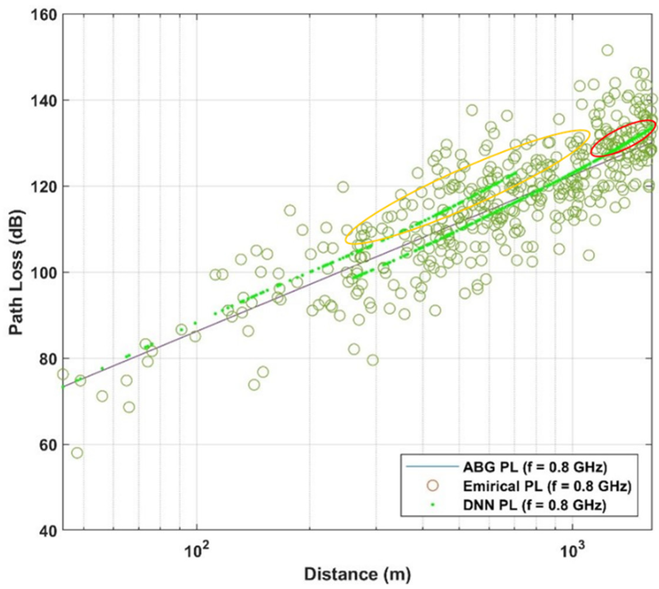
- The performance of the proposed DNN model for multi-frequency path loss data is compared to the conventional linear ABG multi-frequency path loss model [4] in terms of prediction error and prediction accuracy.
- (3)
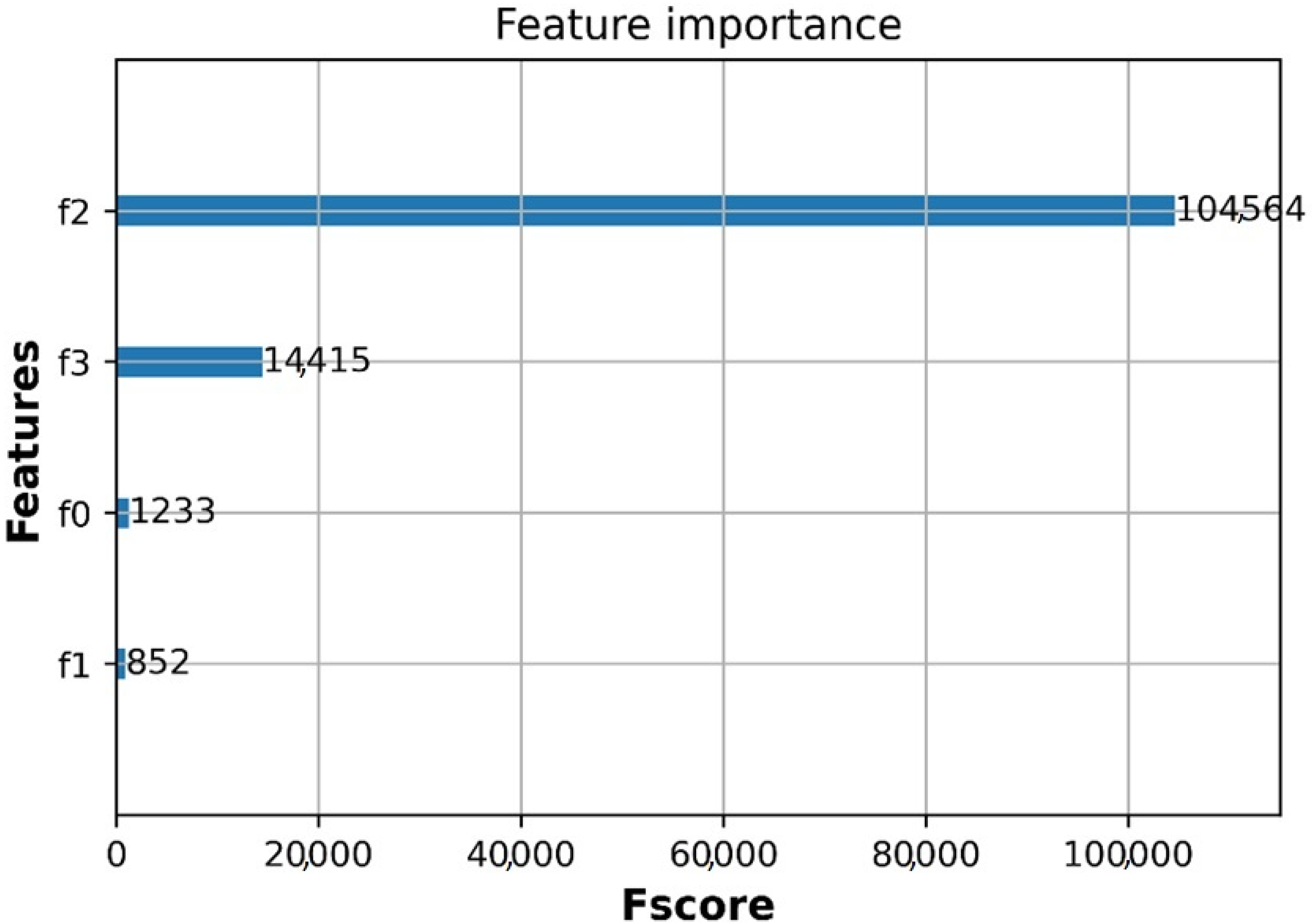
- The paper applied the XGBoost technique to analyze the feature importance of the dataset to observe how much each feature contributes to the prediction model.
- (4)
- The effect of each hyperparameter on the performance of the proposed DNN model in terms of prediction accuracy and the prediction error is also investigated.
2. Proposed Model
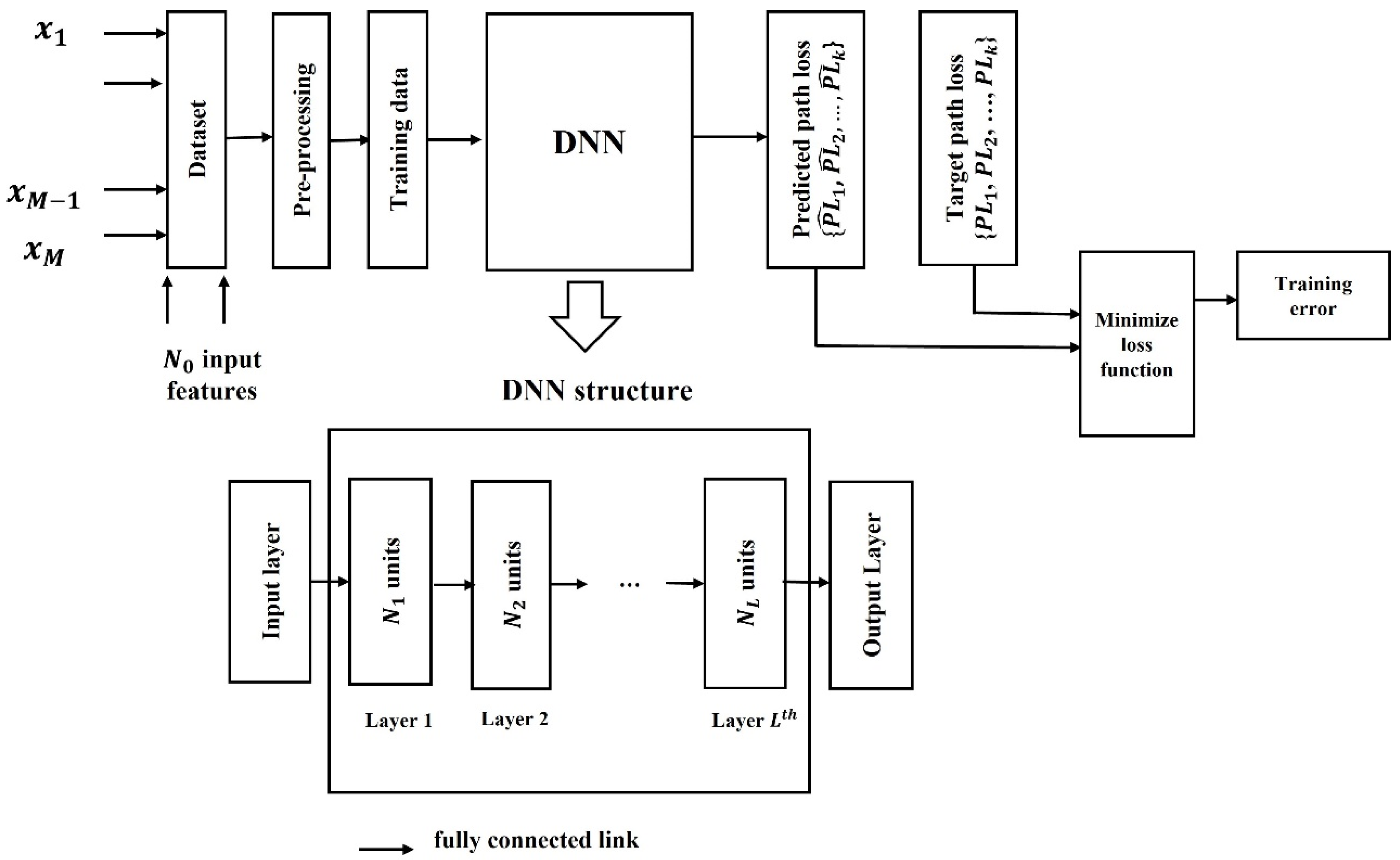
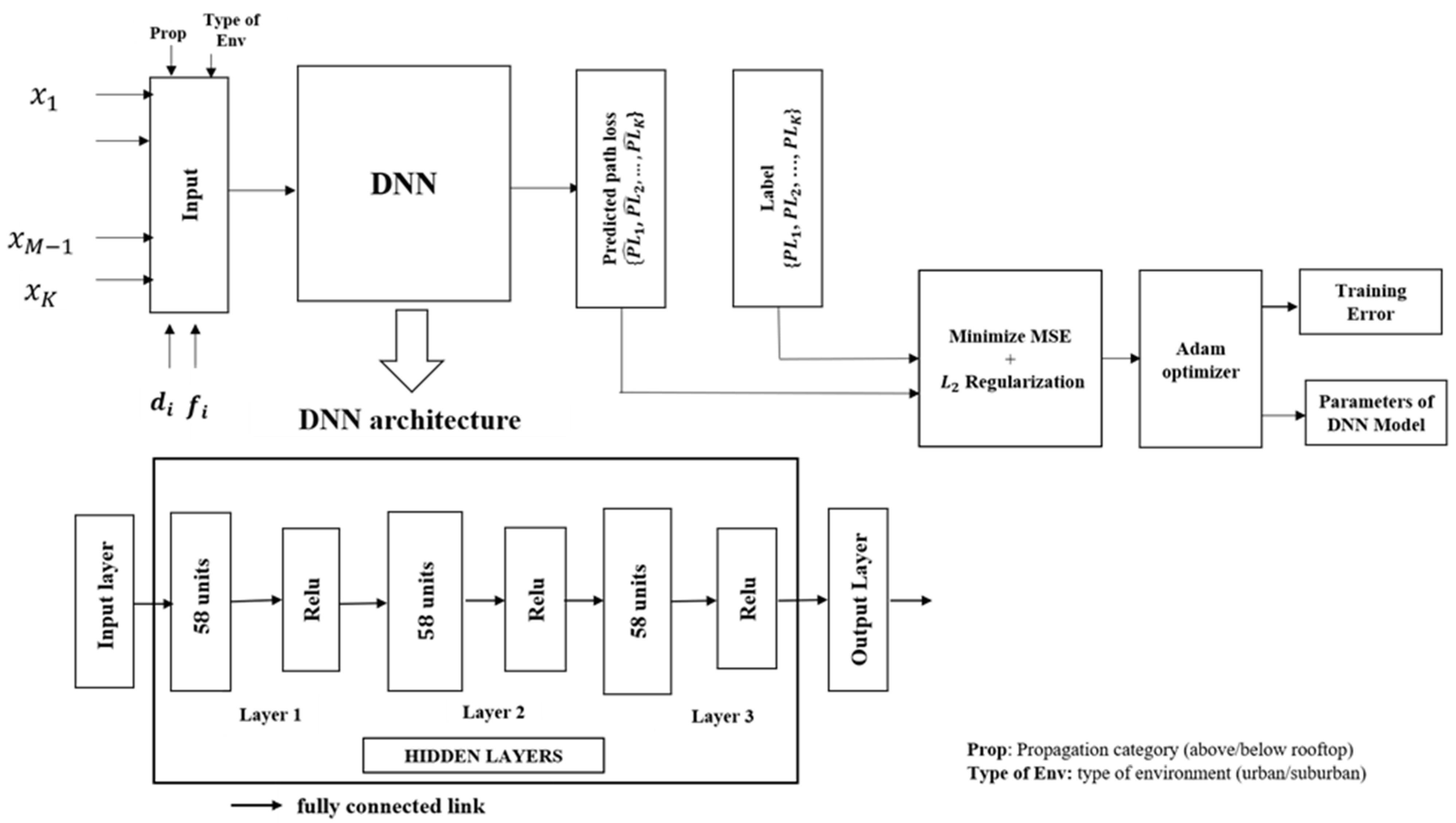
2.1. Architecture
2.2. Hyperparameters
3. ABG Path Loss Model and Parameters
4. Use Case and Dataset
5. DNN Model Training and Validation
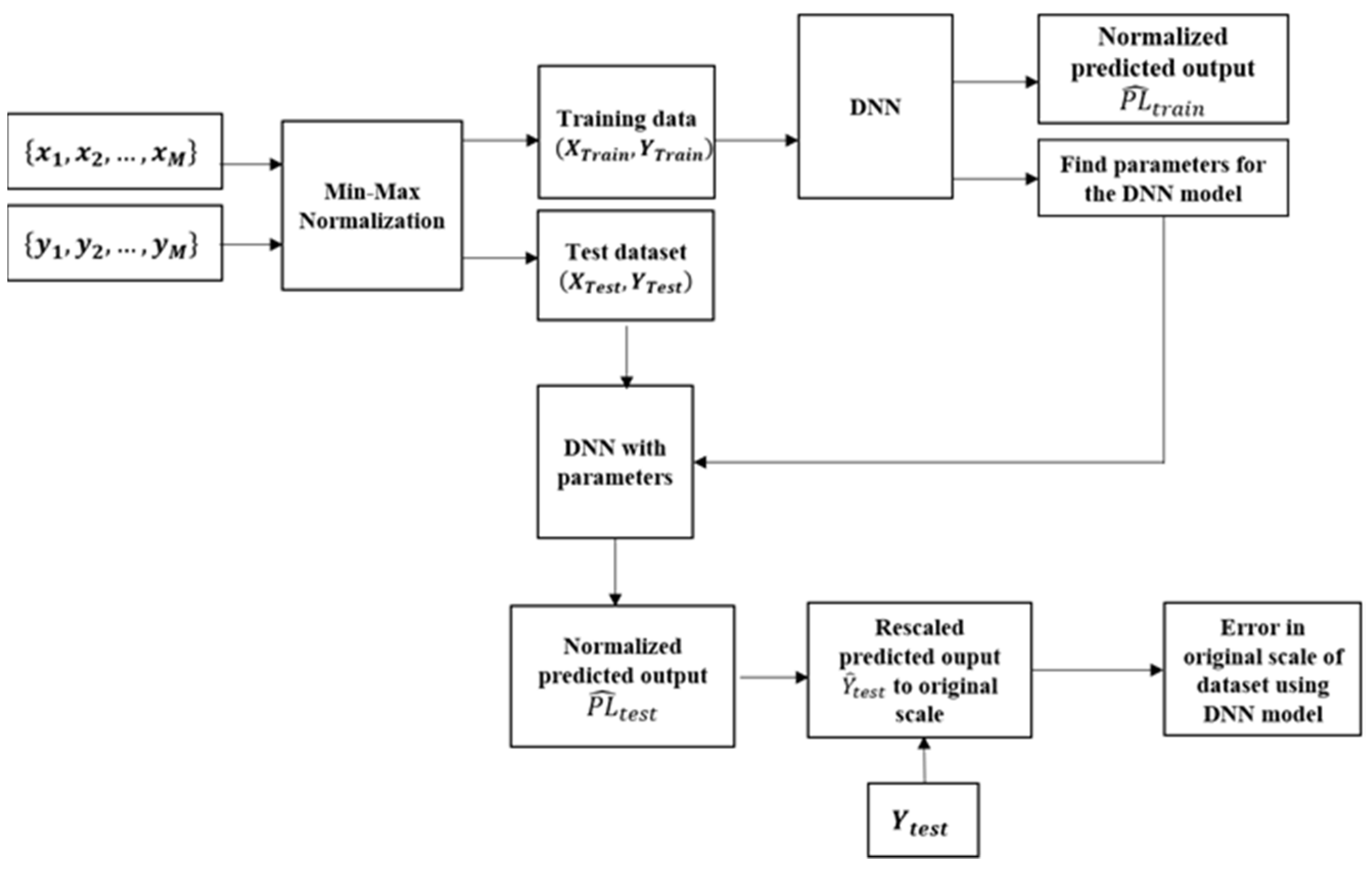
5.1. Dataset Preparation
5.2. Analysis of Feature Importance on the Prediction Using XGBoost Algorithm
5.3. Performance Metrics
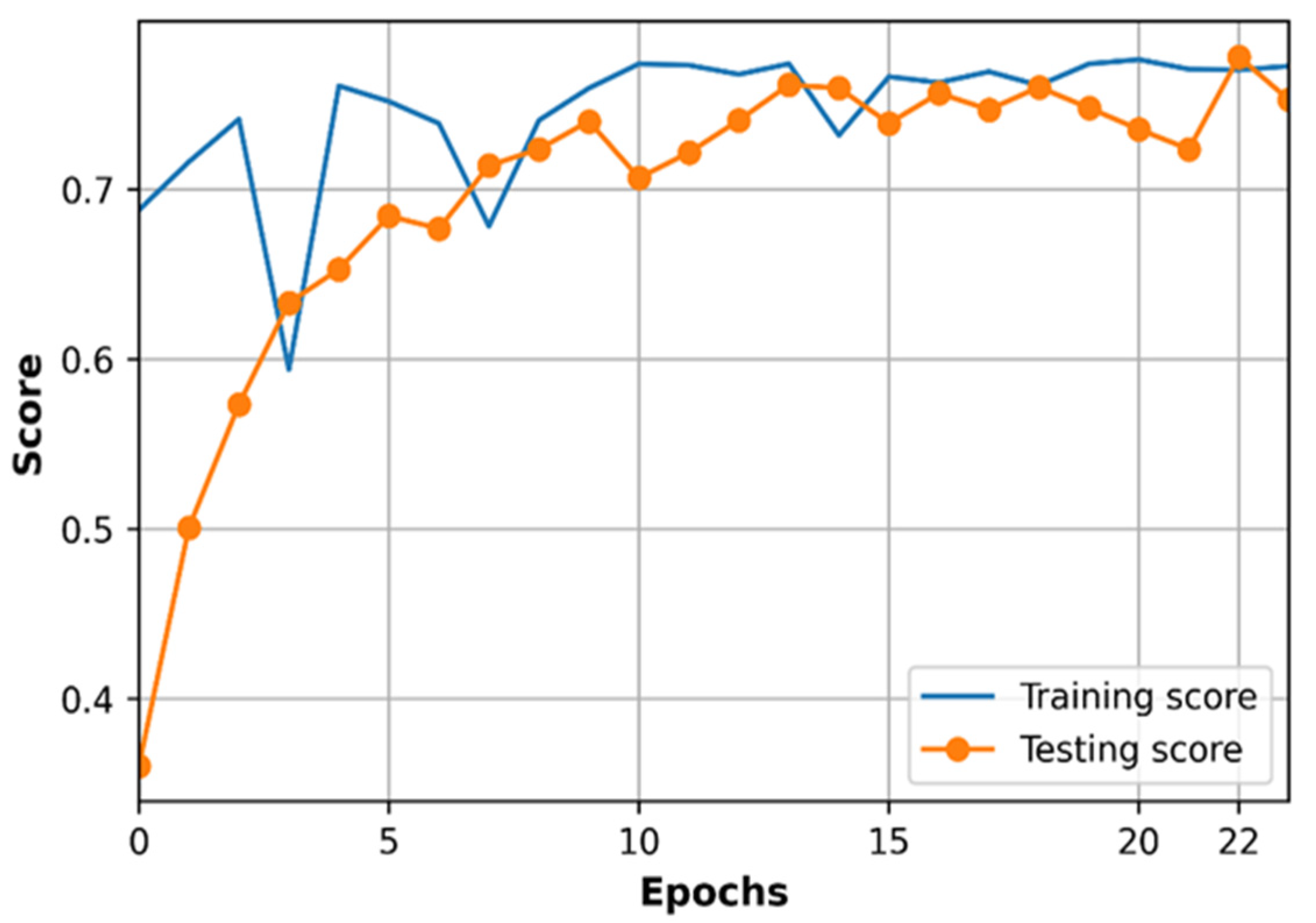
5.4. Training of Proposed DNN Model
5.5. Testing DNN Model
6. Impact of Hyperparameters on the Proposed Model Performance
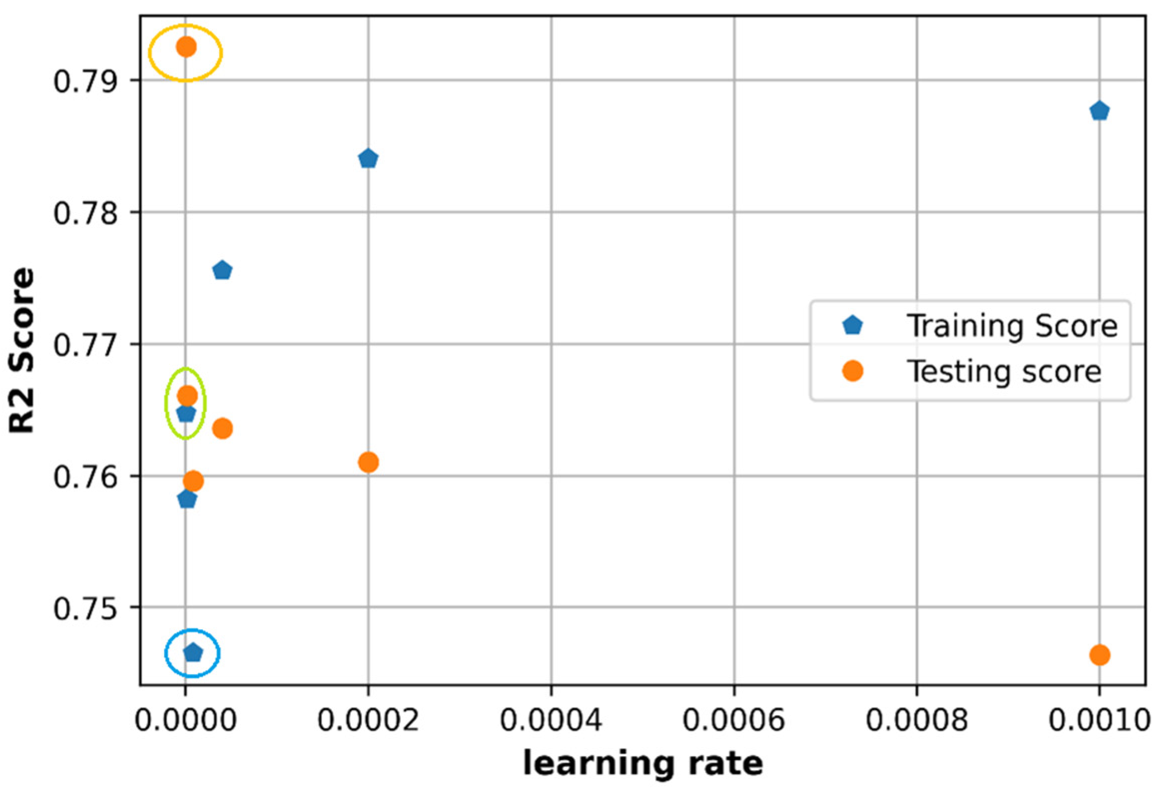
6.1. Effect of Learning Rate
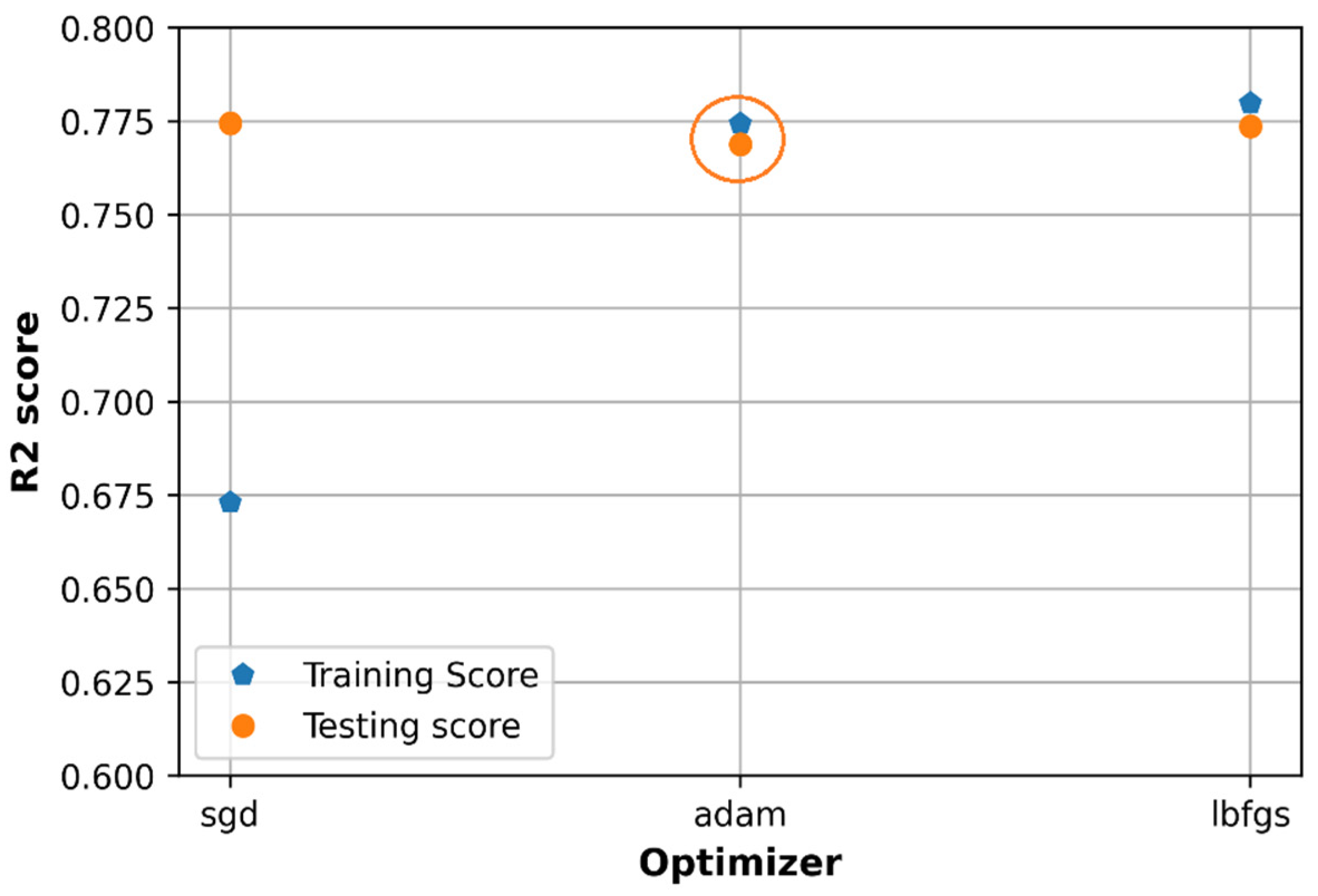
6.2. Effect of Optimizers
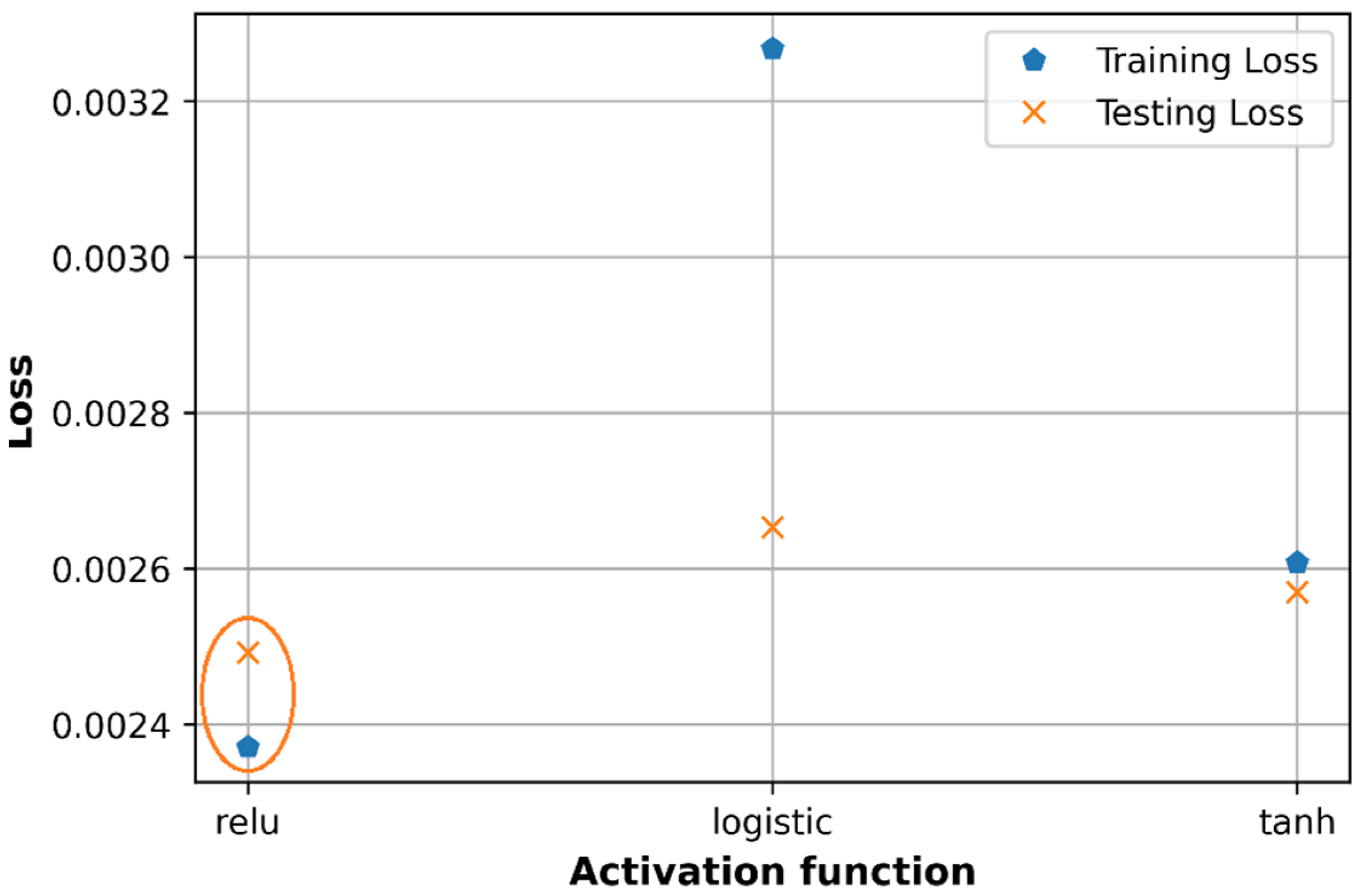
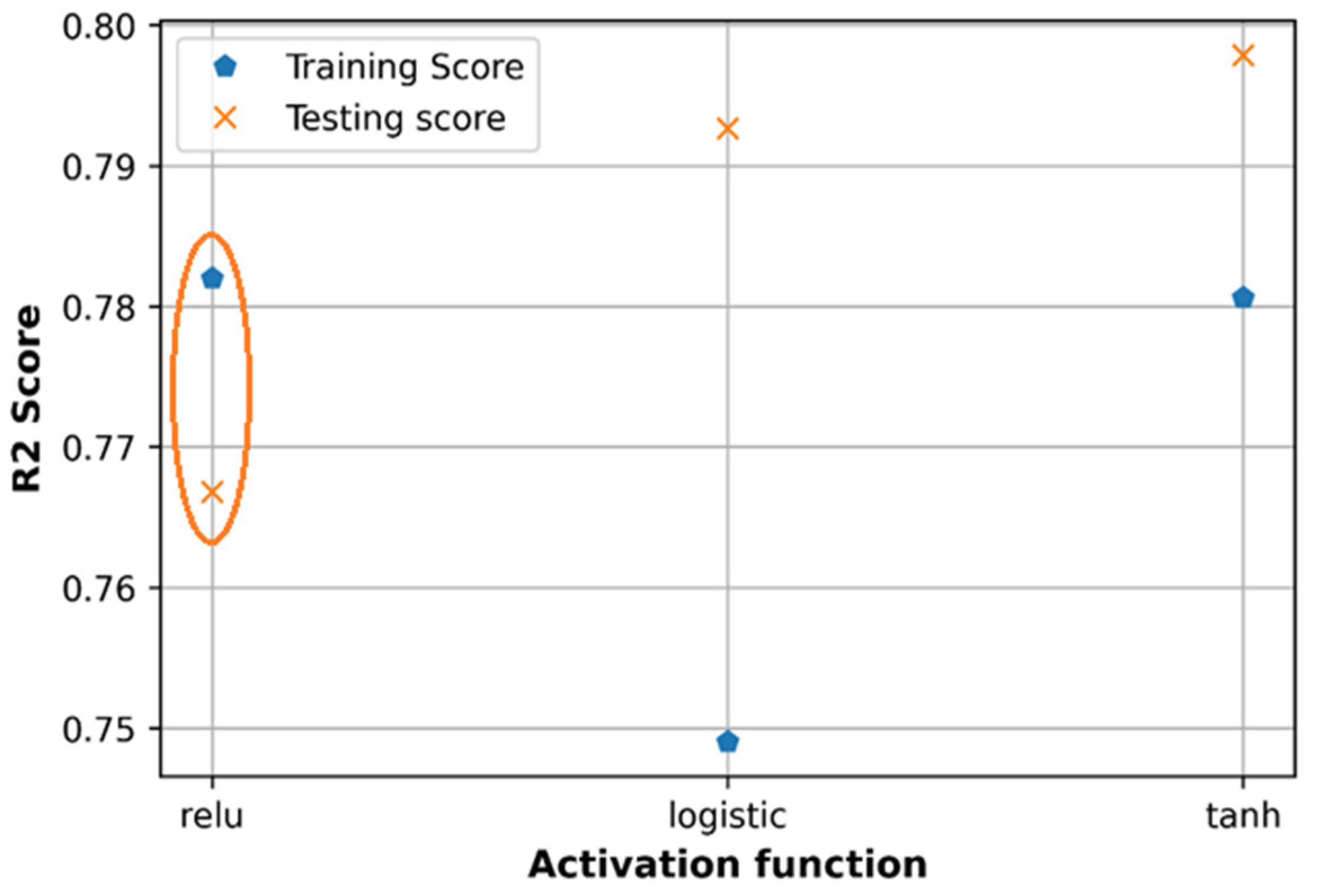
6.3. Effect of Activation Functions
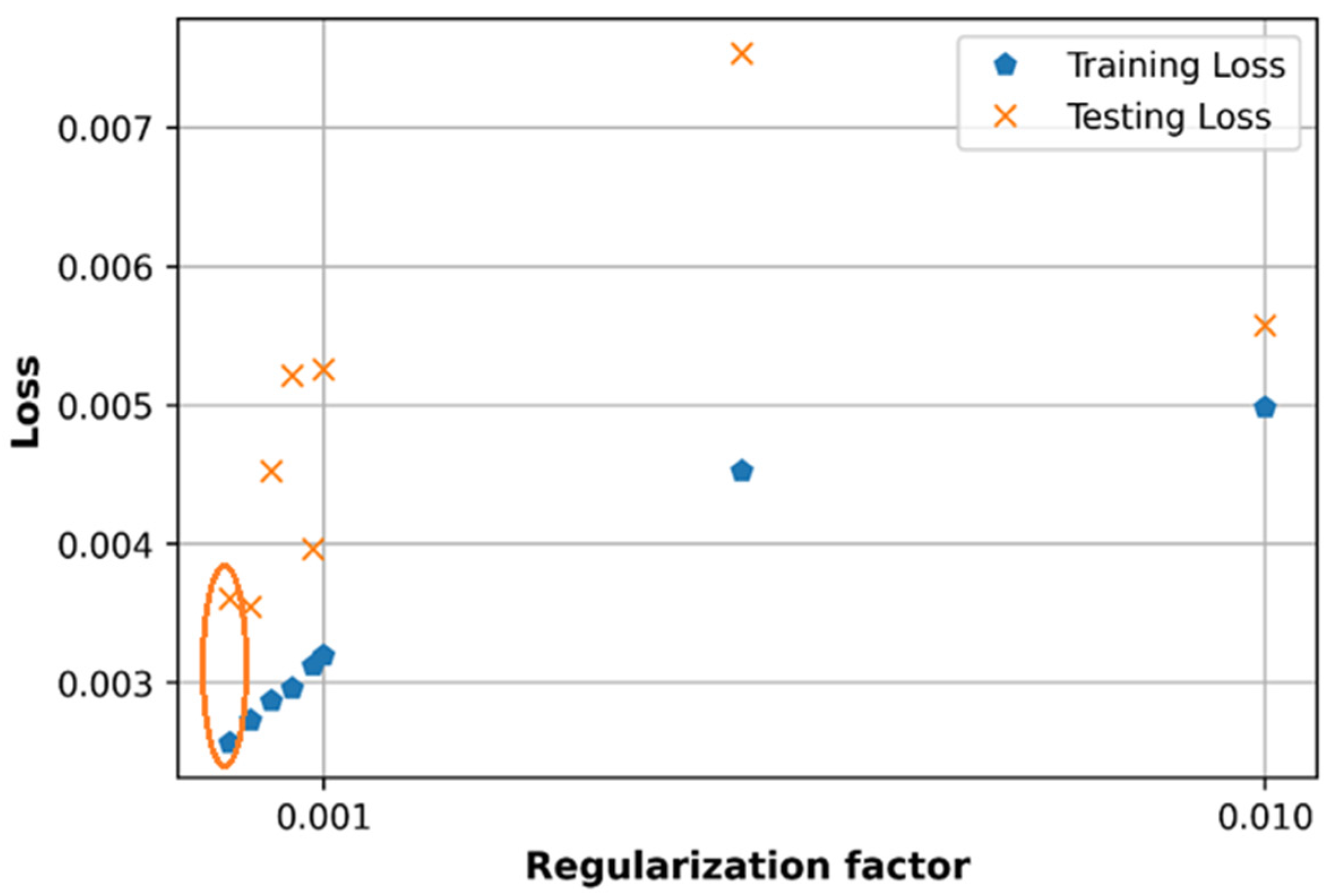
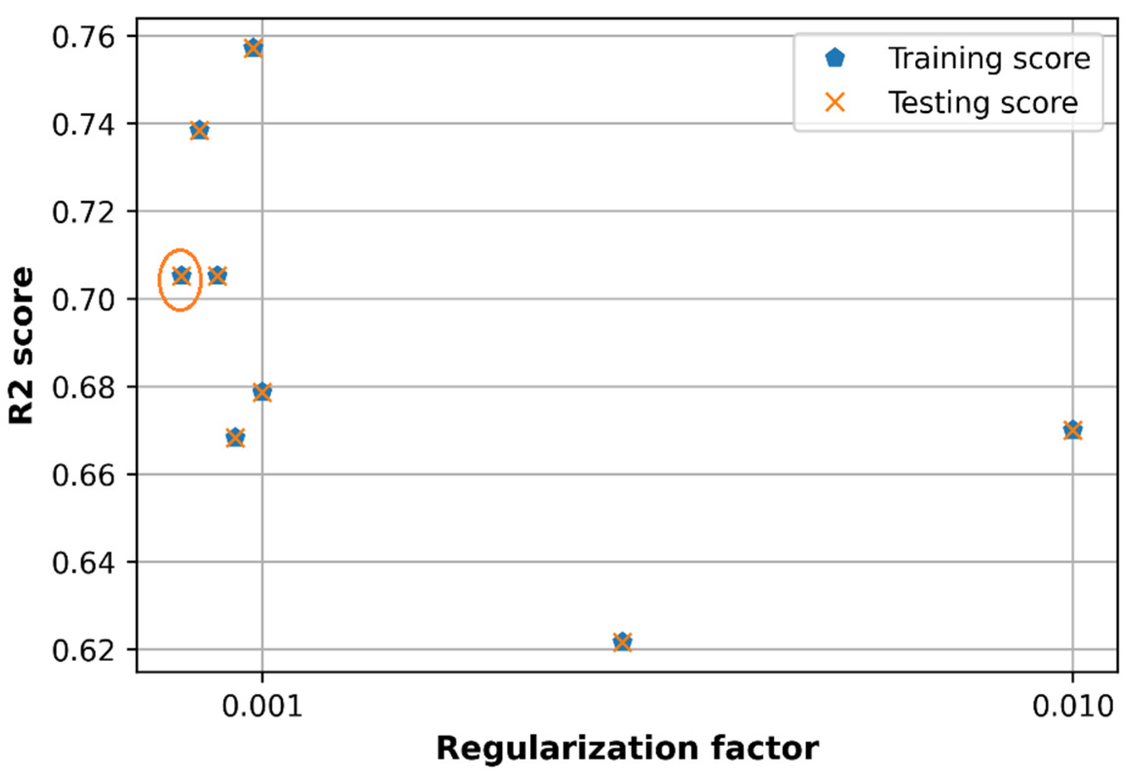
6.4. Effect of Regularization L2 Factor
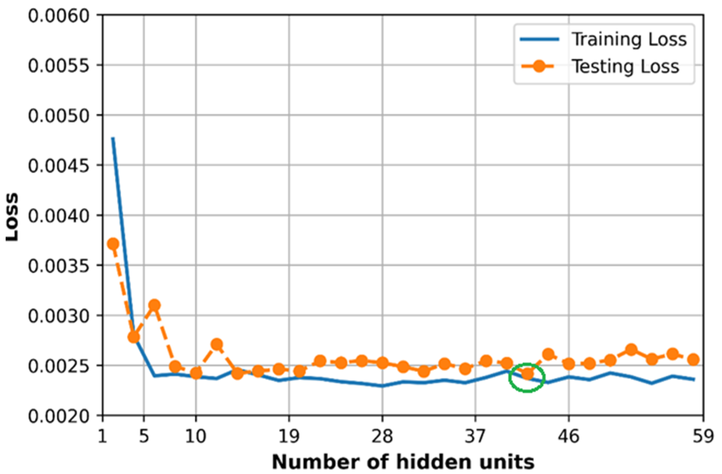
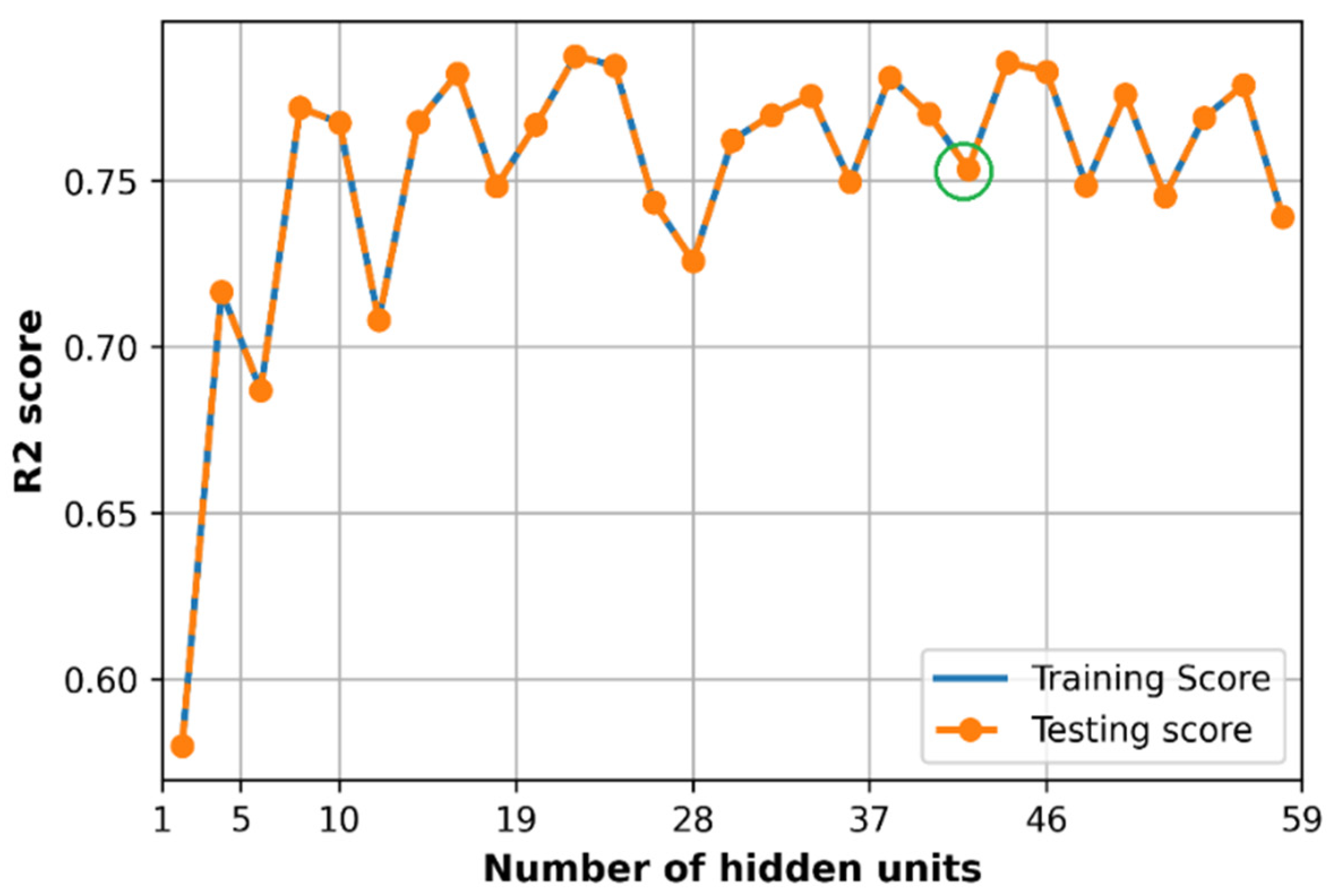
6.5. Effect of Hidden Size
7. Conclusions
Author Contributions
Funding
Conflicts of Interest
References
- Ates, H.F.; Hashir, S.M.; Baykas, T.; Gunturk, B.K. Path Loss Exponent and Shadowing Factor Prediction from Satellite Images Using Deep Learning. IEEE Access 2019, 7, 101366–101375. [Google Scholar] [CrossRef]
- Huang, J.; Cao, Y.; Raimundo, X.; Cheema, A.; Salous, S. Rain Statistics Investigation and Rain Attenuation Modeling for Millimeter Wave Short-Range Fixed Links. IEEE Access 2019, 7, 156110–156120. [Google Scholar] [CrossRef]
- Faruk, N.; Popoola, S.I.; Surajudeen-Bakinde, N.T.; Oloyede, A.A.; Abdulkarim, A.; Olawoyin, L.A.; Ali, M.; Calafate, C.T.; Atayero, A.A. Path Loss Predictions in the VHF and UHF Bands within Urban Environments: Experimental Investigation of Empirical, Heuristics and Geospatial Models. IEEE Access 2019, 7, 77293–77307. [Google Scholar] [CrossRef]
- MacCartney, G.R.; Rappaport, T.S.; Sun, S.; Deng, S. Indoor office wideband millimeter-wave propagation measurements and channel models at 28 and 73 GHz for Ultra-Dense 5G Wireless Networks. IEEE Access 2015, 3, 2388–2424. [Google Scholar] [CrossRef]
- Turan, B.; Coleri, S. Machine Learning Based Channel Modeling for Vehicular Visible Light Communication. arXiv 2020, arXiv:2002.03774. [Google Scholar]
- Phillips, C.; Sicker, D.; Grunwald, D. A Survey of Wireless Path Loss Prediction and Coverage Mapping Methods. IEEE Commun. Surv.Tutor. 2013, 15, 255–270. [Google Scholar] [CrossRef]
- Park, C.; Tettey, D.K.; Jo, H.-S. Artificial Neural Network Modeling for Path Loss Prediction in Urban Environments. arXiv 2019, arXiv:1904.02383. [Google Scholar]
- Aldossari, S.; Chen, K.C. Predicting the Path Loss of Wireless Channel Models Using Machine Learning Techniques in MmWave Urban Communications. arXiv 2020, arXiv:2005.00745. [Google Scholar]
- Zhang, Y.; Wen, J.; Yang, G.; He, Z.; Wang, J. Path Loss Prediction Based on Machine Learning: Principle, Method, and Data Expansion. Appl. Sci. 2019, 9, 1908. [Google Scholar] [CrossRef] [Green Version]
- Nguyen, D.C.; Cheng, P.; DIng, M.; Lopez-Perez, D.; Pathirana, P.N.; Li, J.; Seneviratne, A.; Li, Y.; Poor, H.V. Enabling AI in Future Wireless Networks: A Data Life Cycle Perspective. IEEE Commun. Surv. Tutor. 2021, 23, 553–595. [Google Scholar] [CrossRef]
- Zhang, R.; Wang, J.; Guo, Q.; Wang, D.; Zhong, Z.; Li, C. Model accuracy and sensitivity assessment based on dual-band large-scale channel measurement. In Proceedings of the 2018 24th Asia-Pacific Conference on Communications (APCC), Ningbo, China, 12–14 November 2018; pp. 558–563. [Google Scholar] [CrossRef]
- Fernandes, L.C.; José, A.; Soares, M. Simplified Characterization of the Urban Propagation Environment for Path Loss Calculation. IEEE Antennas Wirel. Propag Lett. 2010, 9, 24–27. [Google Scholar] [CrossRef]
- Ferreira, G.P.; Matos, L.J.; Silva, J.M.M. Improvement of Outdoor Signal Strength Prediction in UHF Band by Artificial Neural Network. IEEE Trans. Antennas Propag. 2016, 64, 5404–5410. [Google Scholar] [CrossRef]
- Kalakh, M.; Kandil, N.; Hakem, N. Neural networks model of an UWB channel path loss in a mine environment. In Proceedings of the 2012 IEEE 75th Vehicular Technology Conference (VTC Spring), Yokohama, Japan, 6–9 May 2012. [Google Scholar] [CrossRef]
- Popoola, S.I.; Jefia, A.; Atayero, A.A.; Kingsley, O.; Faruk, N.; Oseni, O.F.; Abolade, R.O. Determination of neural network parameters for path loss prediction in very high frequency wireless channel. IEEE Access 2019, 7, 150462–150483. [Google Scholar] [CrossRef]
- Olajide, O.Y.; Yerima, S.M. Channel Path-Loss Measurement and Modeling in Wireless Data Network (IEEE 802.11n) Using Artificial Neural Network. Eur. J. Electr. Eng. Comput. Sci. 2020, 4, 1–7. [Google Scholar] [CrossRef]
- Thrane, J.; Zibar, D.; Christiansen, H.L. Model-aided deep learning method for path loss prediction in mobile communication systems at 2.6 GHz. IEEE Access 2020, 8, 7925–7936. [Google Scholar] [CrossRef]
- Eichie, J.O.; Oyedum, O.D.; Ajewole, M.O.; Aibinu, A.M. Artificial Neural Network model for the determination of GSM Rxlevel from atmospheric parameters. Eng. Sci. Technol. Int. J. 2017, 20, 795–804. [Google Scholar] [CrossRef] [Green Version]
- Popoola, S.I.; Adetiba, E.; Atayero, A.A.; Faruk, N.; Calafate, C.T. Optimal model for path loss predictions using feed-forward neural networks. Cogent Eng. 2018, 5, 1444345. [Google Scholar] [CrossRef]
- Singh, H.; Gupta, S.; Dhawan, C.; Mishra, A. Path Loss Prediction in Smart Campus Environment: Machine Learning-based Approaches. IEEE Veh. Technol. Conf. 2020, 1–5. [Google Scholar] [CrossRef]
- Sotiroudis, S.P. Neural Networks and Random Forests: A Comparison Regarding Prediction of Propagation Path Loss for NB-IoT Networks. In Proceedings of the 2019 8th International Conference on Modern Circuits and Systems Technologies (MOCAST), Thessaloniki, Greece, 13–15 May 2019; pp. 2019–2022. [Google Scholar]
- Suzuki, H. Macrocell Path-Loss Prediction Using Artificial Neural Networks. IEEE Trans. Vehic. Technol. 2010, 59, 2735–2747. [Google Scholar]
- Wen, J.; Zhang, Y.; Yang, G.; He, Z.; Zhang, W. Path Loss Prediction Based on Machine Learning Methods for Aircraft Cabin Environments. IEEE Access 2019, 7, 159251–159261. [Google Scholar] [CrossRef]
- Ayadi, M.; Ben Zineb, A.; Tabbane, S. A UHF Path Loss Model Using Learning Machine for Heterogeneous Networks. IEEE Trans. Antennas Propag. 2017, 65, 3675–3683. [Google Scholar] [CrossRef]
- Jo, H.S.; Park, C.; Lee, E.; Choi, H.K.; Park, J. Path Loss Prediction Based on Machine Learning Techniques: Principal Component Analysis, Artificial Neural Network, and Gaussian Process. Sensors 2020, 20, 1927. [Google Scholar] [CrossRef] [PubMed] [Green Version]
- Zineb, A.B.; Ayadi, M. A Multi-wall and Multi-frequency Indoor Path Loss Prediction Model Using Artificial Neural Networks. Arab. J. Sci. Eng. 2016, 41, 987–996. [Google Scholar] [CrossRef]
- Liu, J.; Jin, X.; Dong, F.; He, L.; Liu, H. Fading channel modelling using single-hidden layer feedforward neural networks. Multidimens. Syst. Signal Process. 2017, 28, 885–903. [Google Scholar] [CrossRef]
- Yu, T.; Zhu, H. Hyper-parameter optimization: A review of algorithms and applications. arXiv 2020, arXiv:2003.05689. [Google Scholar]
- Shrestha, A. Review of Deep Learning Algorithms and Architectures. IEEE Access 2019, 7, 53040–53065. [Google Scholar] [CrossRef]
- Sze, V.; Member, S.; Chen, Y.; Member, S.; Yang, T. Efficient Processing of Deep Neural Networks: A Tutorial and Survey. Proc. IEEE 2017, 105, 2295–2329. [Google Scholar] [CrossRef] [Green Version]
- Sarker, I.H. Deep Cybersecurity: A Comprehensive Overview from Neural Network and Deep Learning Perspective. SN Comput. Sci. 2021, 2, 154. [Google Scholar] [CrossRef]
- Mao, Q.; Hu, F.; Hao, Q. Deep learning for intelligent wireless networks: A comprehensive survey. IEEE Commun. Surv. Tutor. 2018, 20, 2595–2621. [Google Scholar] [CrossRef]
- Kulin, M.; Kazaz, T.; Moerman, I.; de Poorter, E. A survey on machine learning-based performance improvement of wireless networks: PHY, MAC and Network layer. arXiv 2020, arXiv:2003.05689. [Google Scholar]
- Liao, R.F.; Wen, H.; Wu, J.; Song, H.; Pan, F.; Dong, L. The Rayleigh Fading Channel Prediction via Deep Learning. Wirel. Commun. Mob. Comput. 2018, 2018, 6497340. [Google Scholar] [CrossRef]
- Bergstra, J.; Bengio, Y. Random search for hyper-parameter optimization. J. Mach. Learn. Res. 2012, 13, 281–305. [Google Scholar]
- Salous, S.; Lee, J.; Kim, M.D.; Sasaki, M.; Yamada, W.; Raimundo, X.; Cheema, A.A. Radio propagation measurements and modeling for standardization of the site general path loss model in International Telecommunications Union recommendations for 5G wireless networks. Radio Sci. 2020, 55, 1–12. [Google Scholar] [CrossRef] [Green Version]
- Brownlee, J. XGboost with python Gradient boosted trees with XGBoost and scikit-learn. Acta Univ. Agric. Silvic. Mendel. Brun. 2015, 53, 1689–1699. [Google Scholar]
- Niu, Y. Walmart Sales Forecasting using XGBoost algorithm and Feature engineering. In Proceedings of the 2020 International Conference on Big Data and Artificial Intelligence and Software Engineering, ICBASE, Bangkok, Thailand, 30 October–1 November 2020; pp. 458–461. [Google Scholar]
- Ouadjer, Y. Feature Importance Evaluation of Smartphone Touch Gestures for Biometric Authentication. In Proceedings of the 2020 2nd International Workshop on Human-Centric Smart Environments for Health and Well-being (IHSH), Boumerdes, Algeria, 9–10 February 2021; pp. 103–107. [Google Scholar]
- Zappone, A.; Di Renzo, M.; Debbah, M. Wireless networks design in the era of deep learning: Model-based, AI-based, or both? IEEE Trans. Commun. 2019, 67, 7331–7376. [Google Scholar] [CrossRef] [Green Version]
- Qualcomm Global Update on Spectrum for 4G & 5G. 2020. Available online: https://www.qualcomm.com/media/documents/files/spectrum-for-4g-and-5g.pdf (accessed on 1 June 2021).


| Propagation Category | Environment | Frequency (GHz) | Distance (m) |
|---|---|---|---|
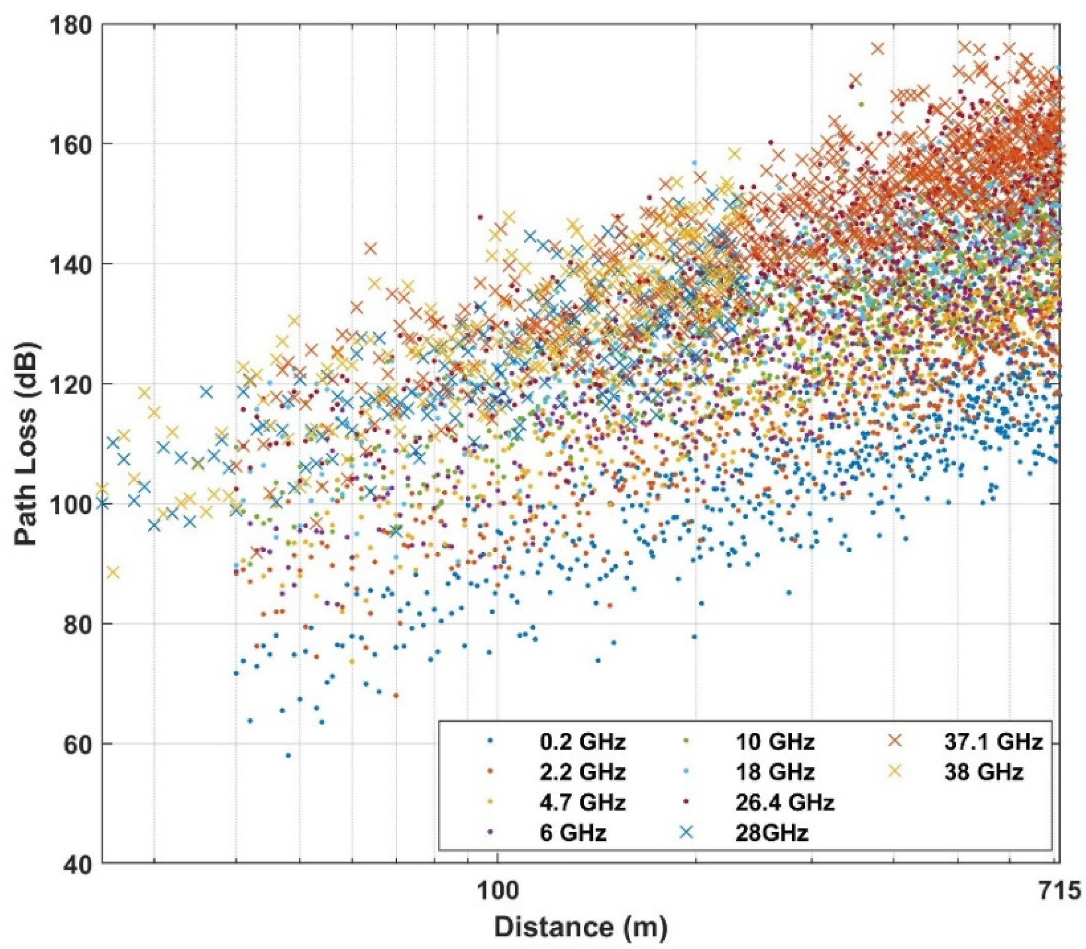
| Below rooftop | Urban high-rise | 0.8, 2.2, 4.7, 6, 10, 18, 26.4, 37.1 | 40–715 |
| 28, 38 | 25–235 | ||
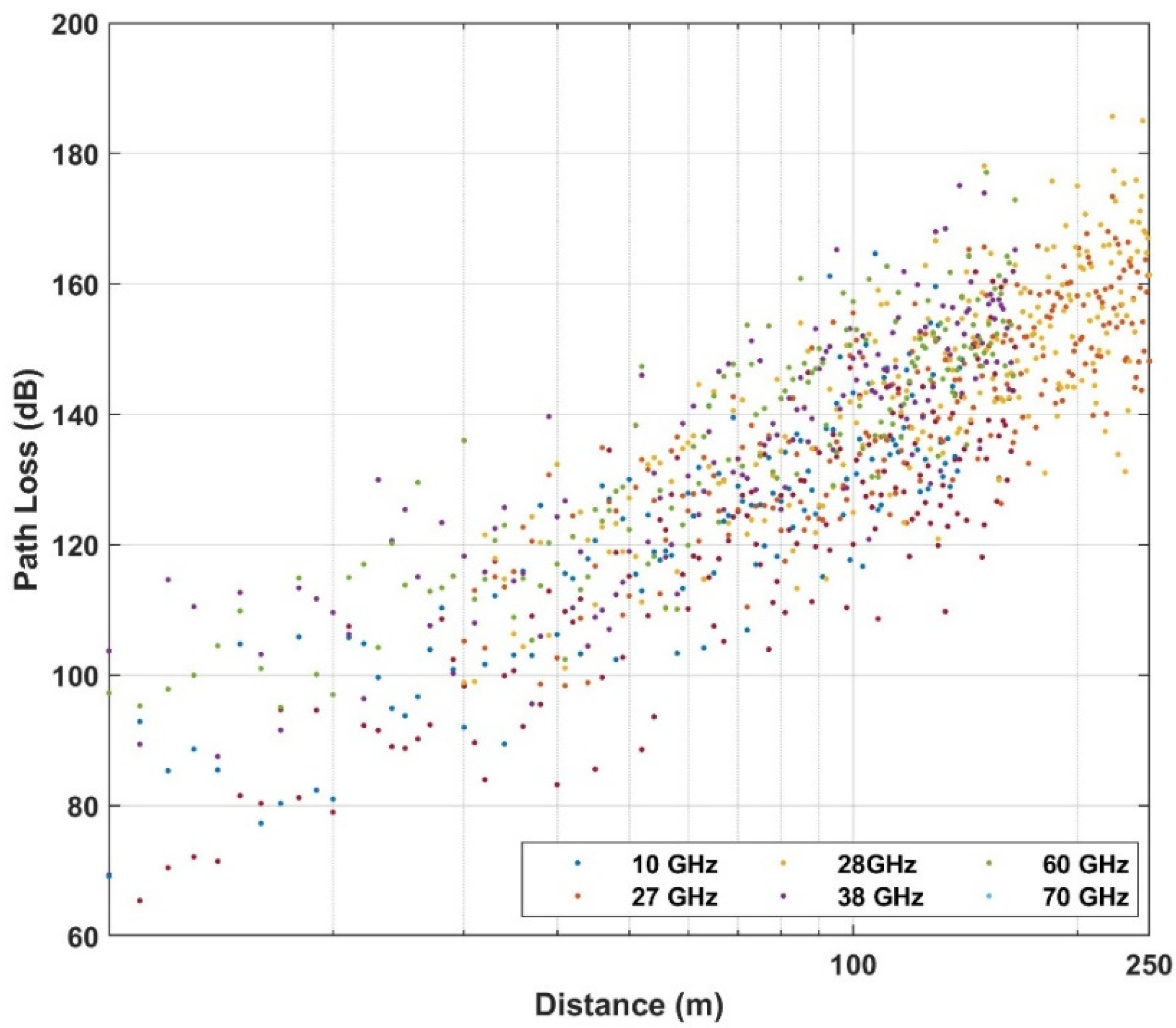
| Urban low-rise (suburban) | 10, 60 | 10–165 | |
| 27 | 10–140 | ||
| 28, 38 | 30–250 | ||
| 70 | 10–170 | ||
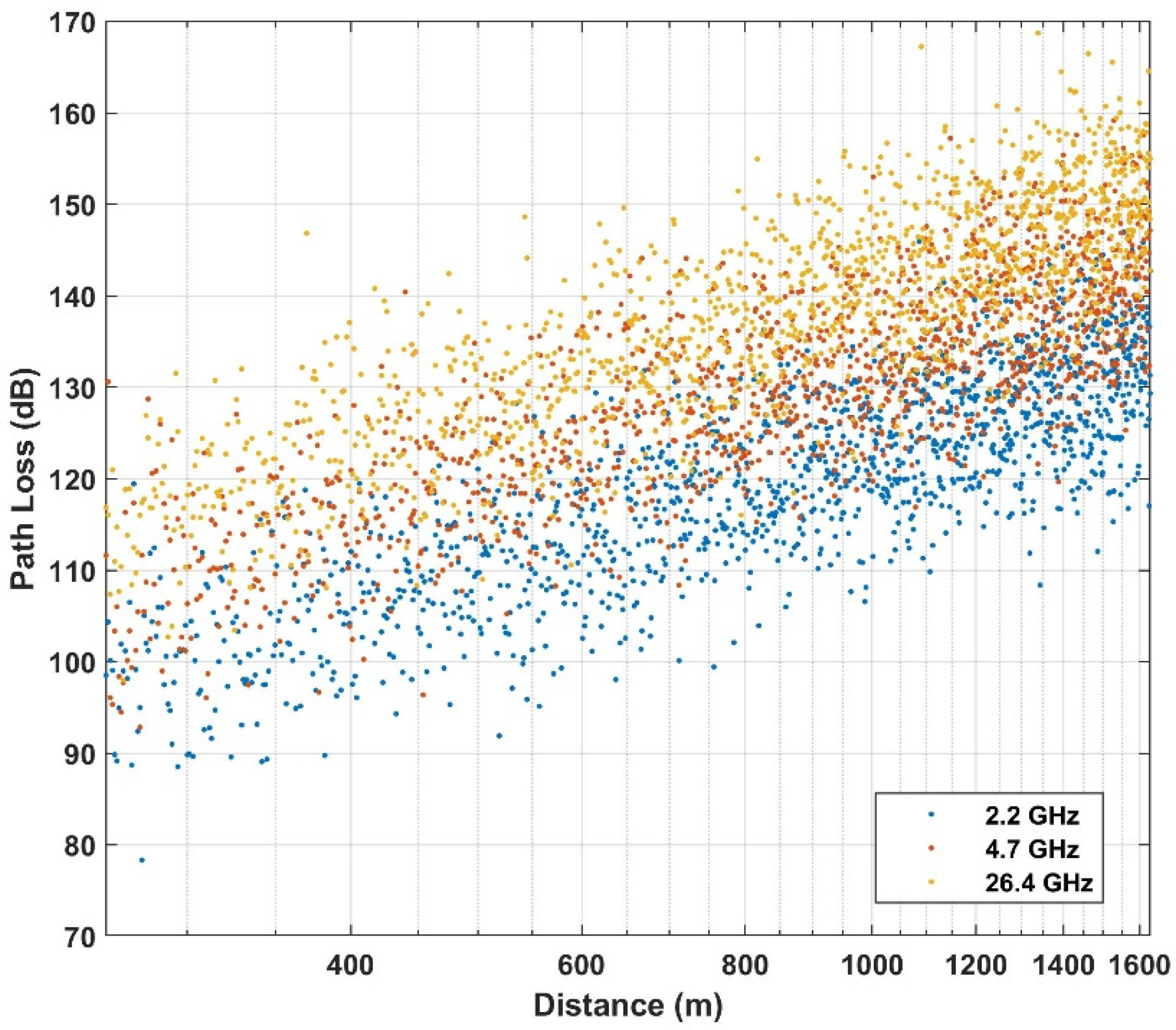
| Above rooftop | Urban high-rise | 2.2, 4.7, 26.4 | 260–1630 |
| Hyperparameters | Values |
|---|---|
| Activation function | Sigmoid logistic, Relu, Tanh |
| Number of units in each hidden layer (same units/neurons in each hidden layer) | Number of hidden layers = [1:1:10] Number of hidden units = [1:1:100] |
| Number of units in each hidden layer (different units/neurons in each hidden layer) | Two hidden layers, number of neurons in each of two hidden layers are permutations in the set Three hidden layers, number of neurons in each of three hidden layers are permutations in the set |
| Optimized algorithms | Stochastic gradient descent, Adam, RMSprop |
| regularization factor | 0.0001, 0.005, 0.001, 0.01 |
| Batch size | 10, 20, 32, 64 |
| Momentum (in case using Adam) | 0.0, 0.2, 0.4, 0.6, 0.8, 0.9 |
| Learning rate | Constant (0.0001) Adaptive (initialized learning rate = 0.001) |
| Hyperparameters | Values |
|---|---|
| Activation function | Relu |
| regularization factor | 0.0001 |
| Batch size | 20 |
| Momentum | 0.4 |
| Hidden layer sizes and units | (58,58,58) |
| Learning rate | Adaptive |
| Optimizer | Adam |
| Performance Metrics [dB] | DNN | ABG |
|---|---|---|
| Max error | 39.07 | 39.92 |
| MSE | 68.48 | 74.56 |
| RMSE | 8.27 | 8.63 |
| MAE | 6.45 | 6.71 |
| R2 score | 0.77 | 0.75 |
Publisher’s Note: MDPI stays neutral with regard to jurisdictional claims in published maps and institutional affiliations. |
© 2021 by the authors. Licensee MDPI, Basel, Switzerland. This article is an open access article distributed under the terms and conditions of the Creative Commons Attribution (CC BY) license (https://creativecommons.org/licenses/by/4.0/).
Share and Cite
Nguyen, C.; Cheema, A.A. A Deep Neural Network-Based Multi-Frequency Path Loss Prediction Model from 0.8 GHz to 70 GHz. Sensors 2021, 21, 5100. https://doi.org/10.3390/s21155100
Nguyen C, Cheema AA. A Deep Neural Network-Based Multi-Frequency Path Loss Prediction Model from 0.8 GHz to 70 GHz. Sensors. 2021; 21(15):5100. https://doi.org/10.3390/s21155100
Chicago/Turabian StyleNguyen, Chi, and Adnan Ahmad Cheema. 2021. "A Deep Neural Network-Based Multi-Frequency Path Loss Prediction Model from 0.8 GHz to 70 GHz" Sensors 21, no. 15: 5100. https://doi.org/10.3390/s21155100
APA StyleNguyen, C., & Cheema, A. A. (2021). A Deep Neural Network-Based Multi-Frequency Path Loss Prediction Model from 0.8 GHz to 70 GHz. Sensors, 21(15), 5100. https://doi.org/10.3390/s21155100