
Methodology of Using Terrain Passability Maps for Planning the Movement of Troops and Navigation of Unmanned Ground Vehicles †


Abstract
:
1. Introduction
1.1. Related Works
1.2. Research Purpose
2. Materials and Methods
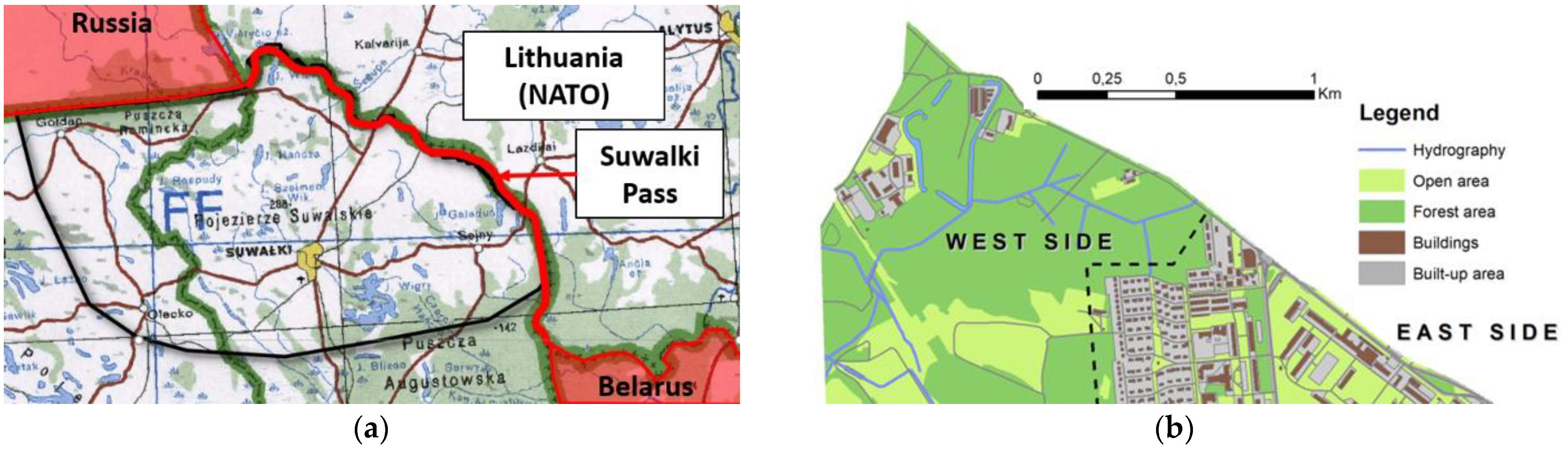
2.1. Area of Research
2.2. Description of the Developed Methodology
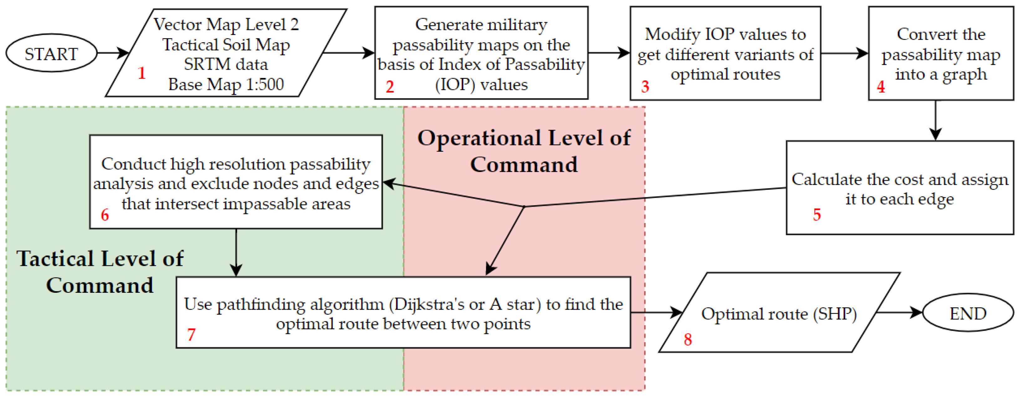
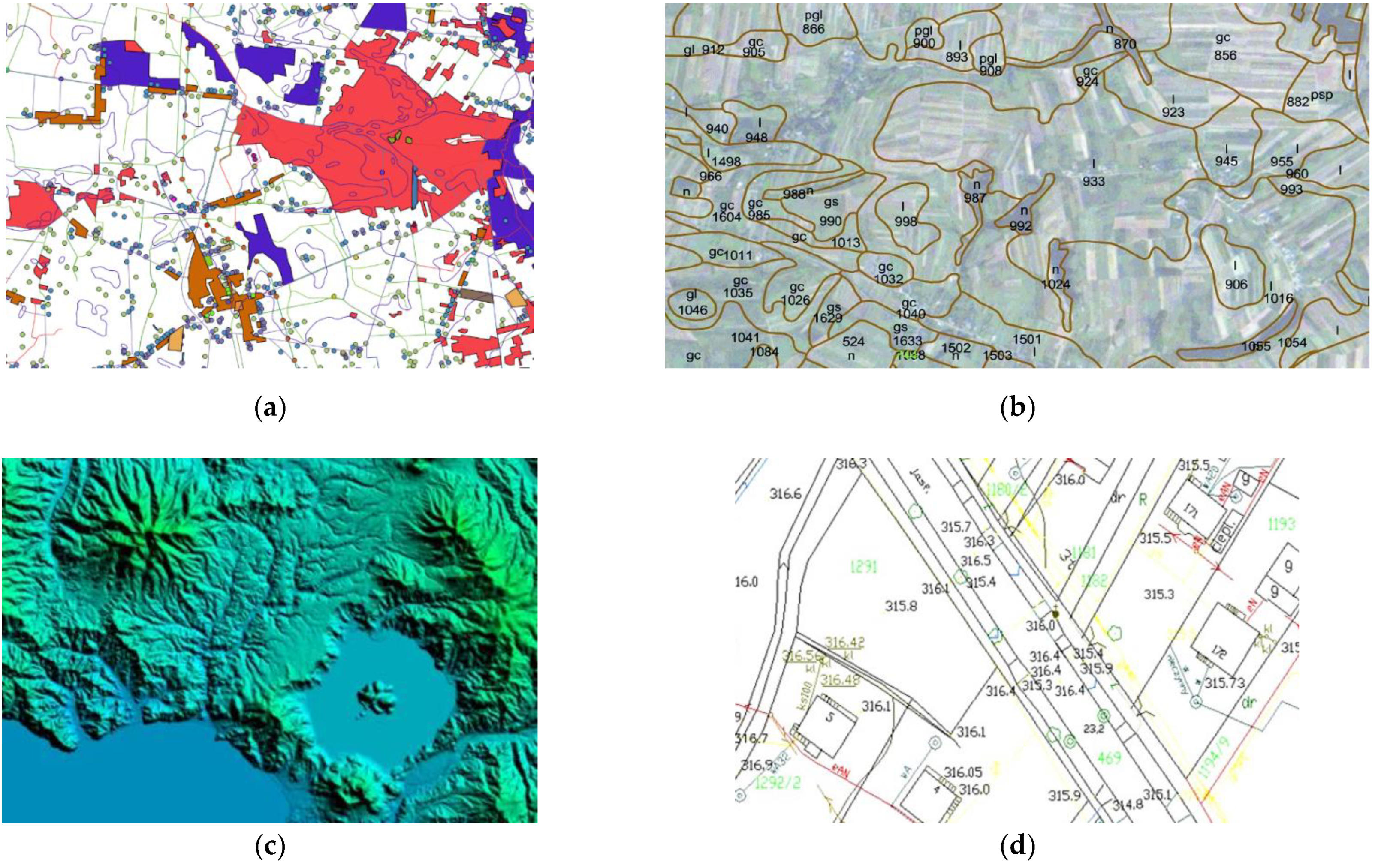
2.2.1. Block No. 1
2.2.2. Block No. 2
2.2.3. Block No. 3
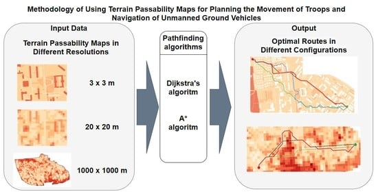
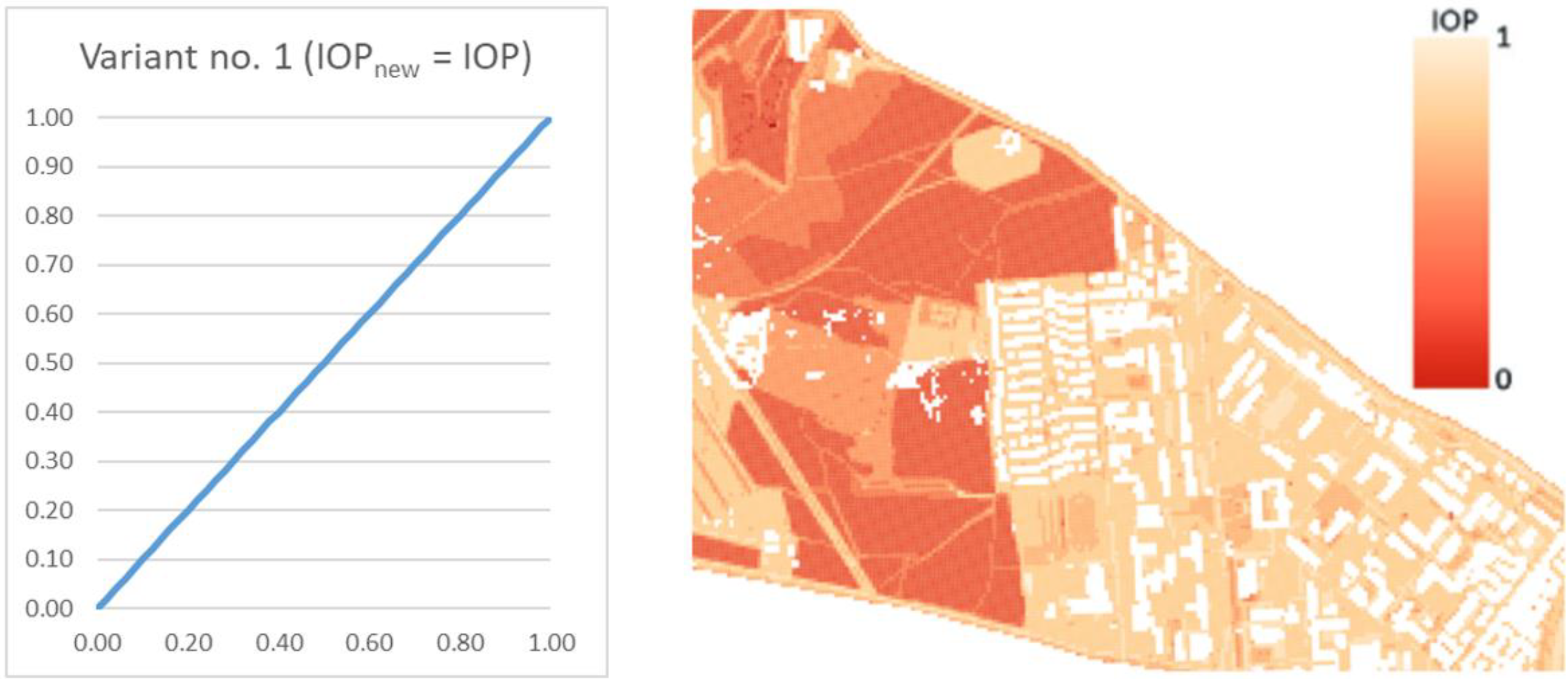
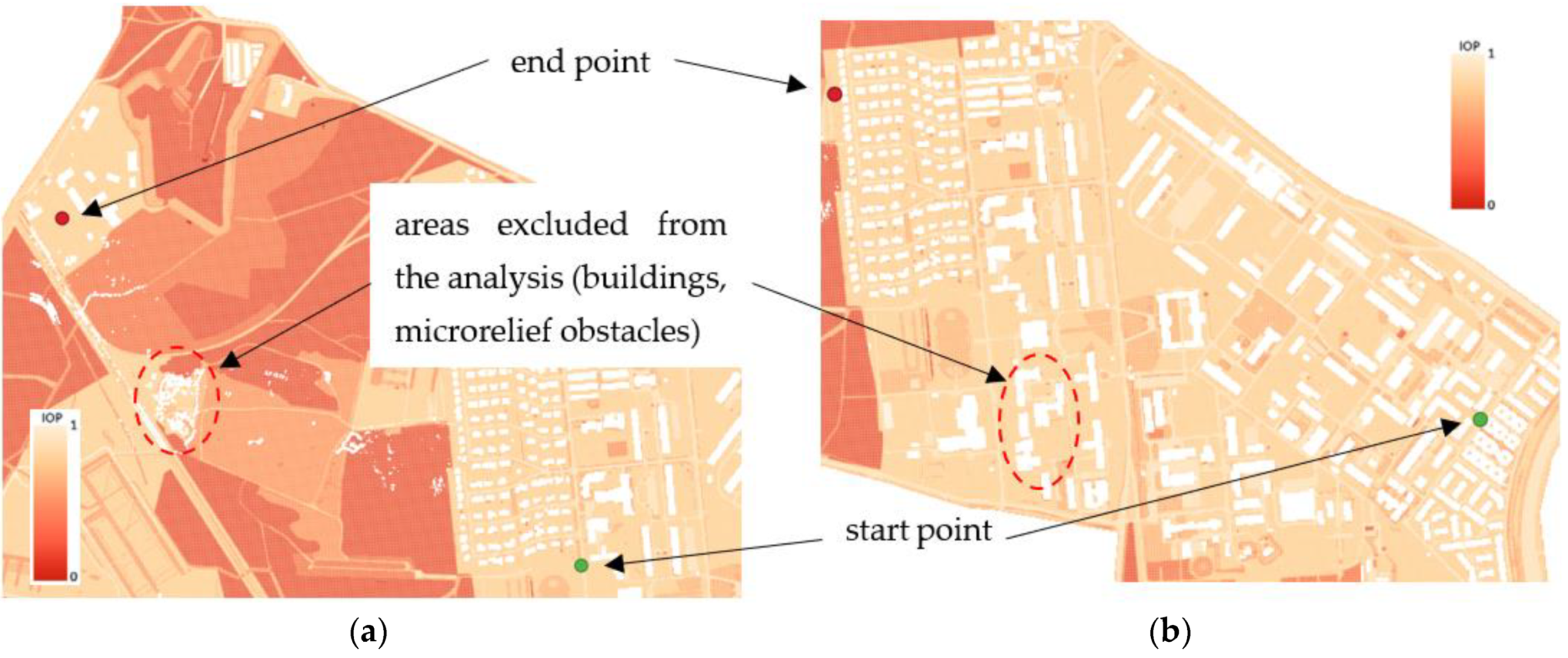
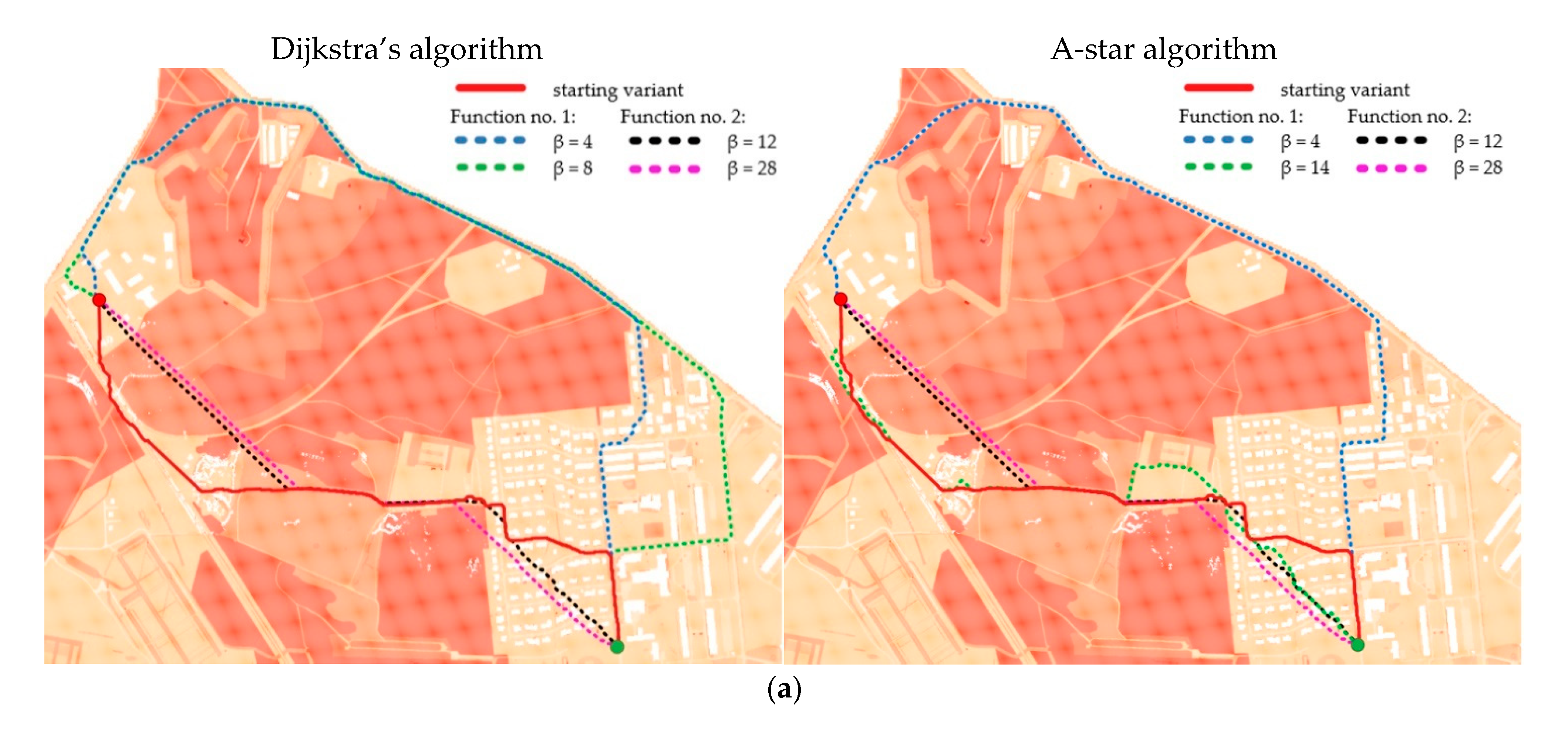
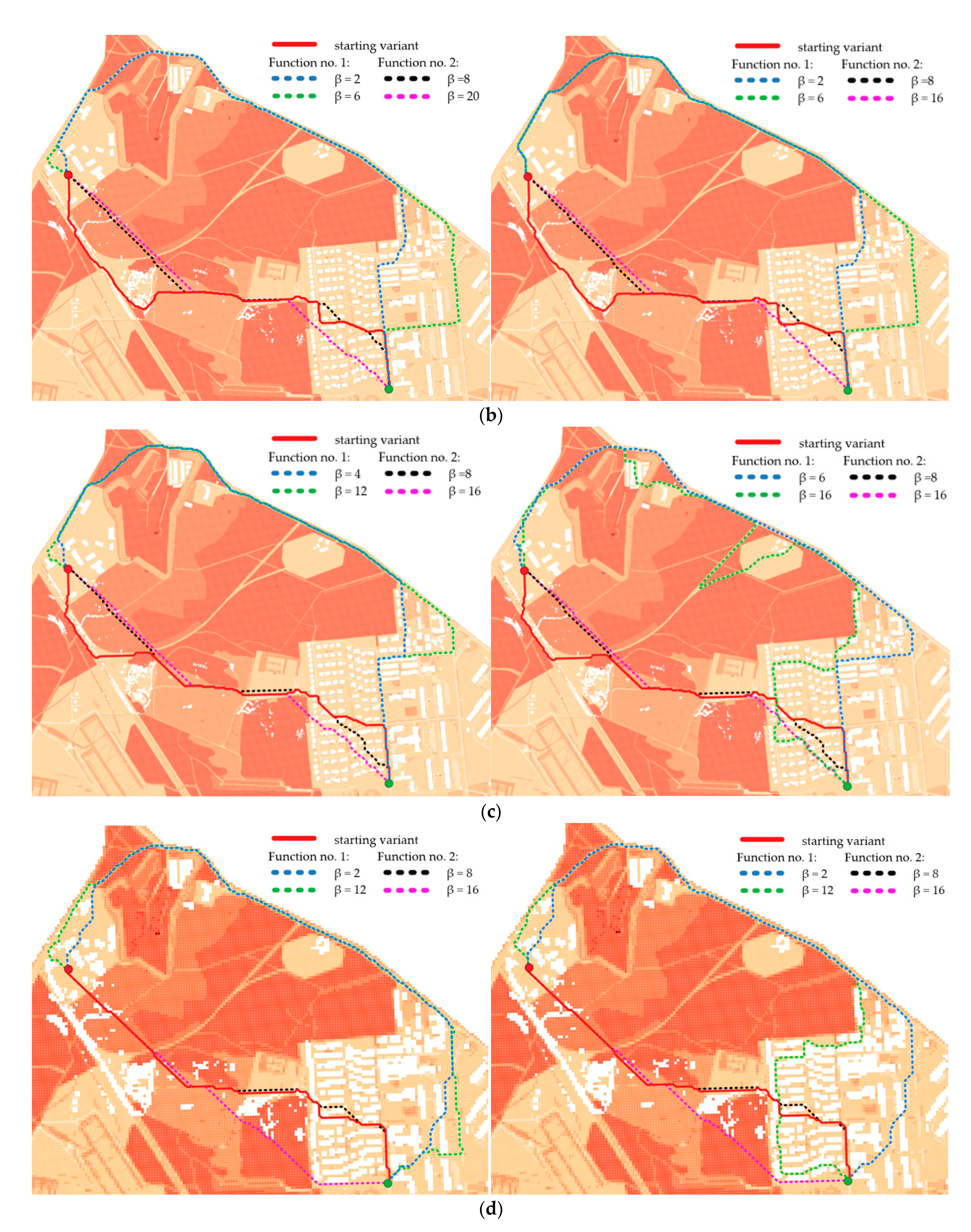
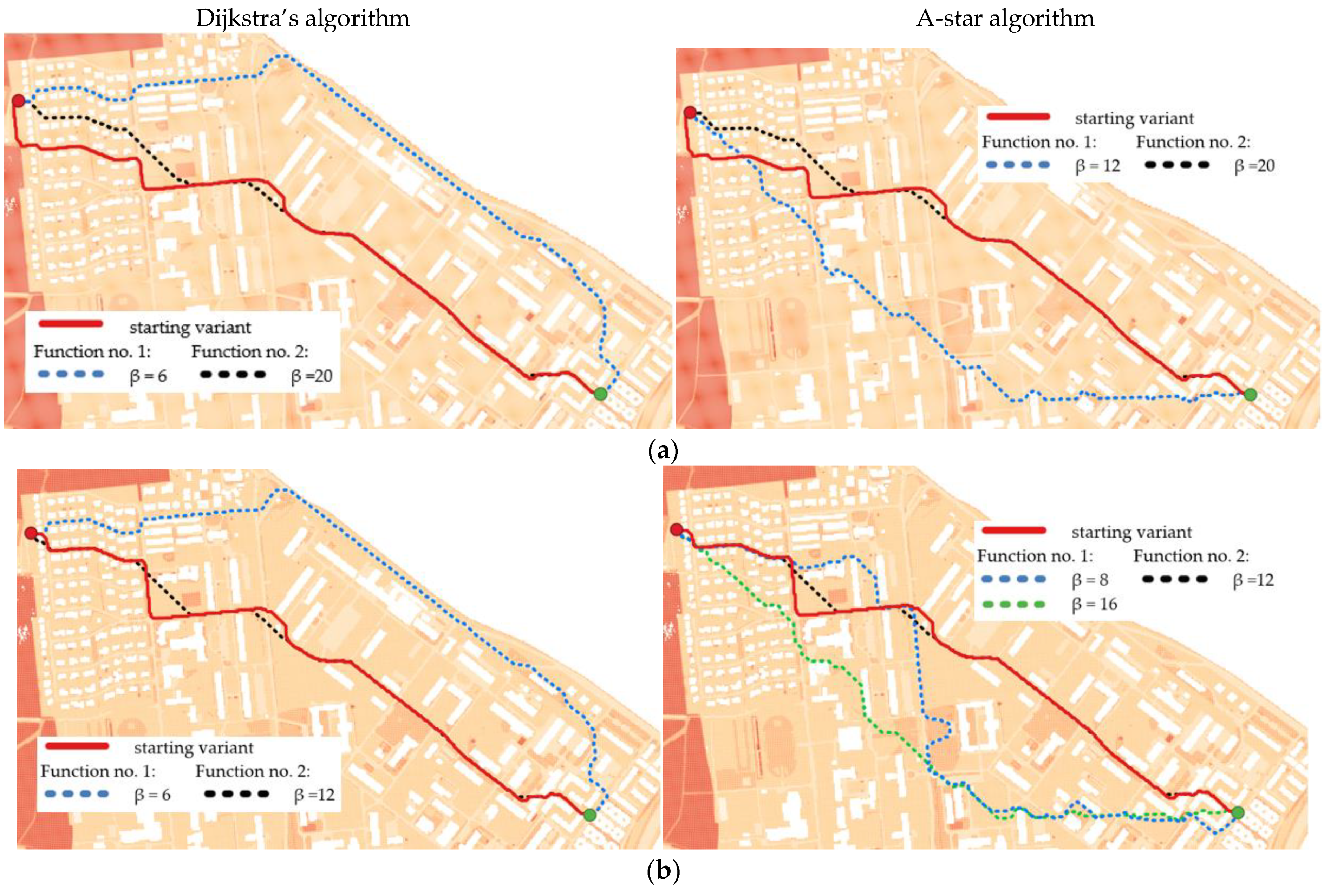
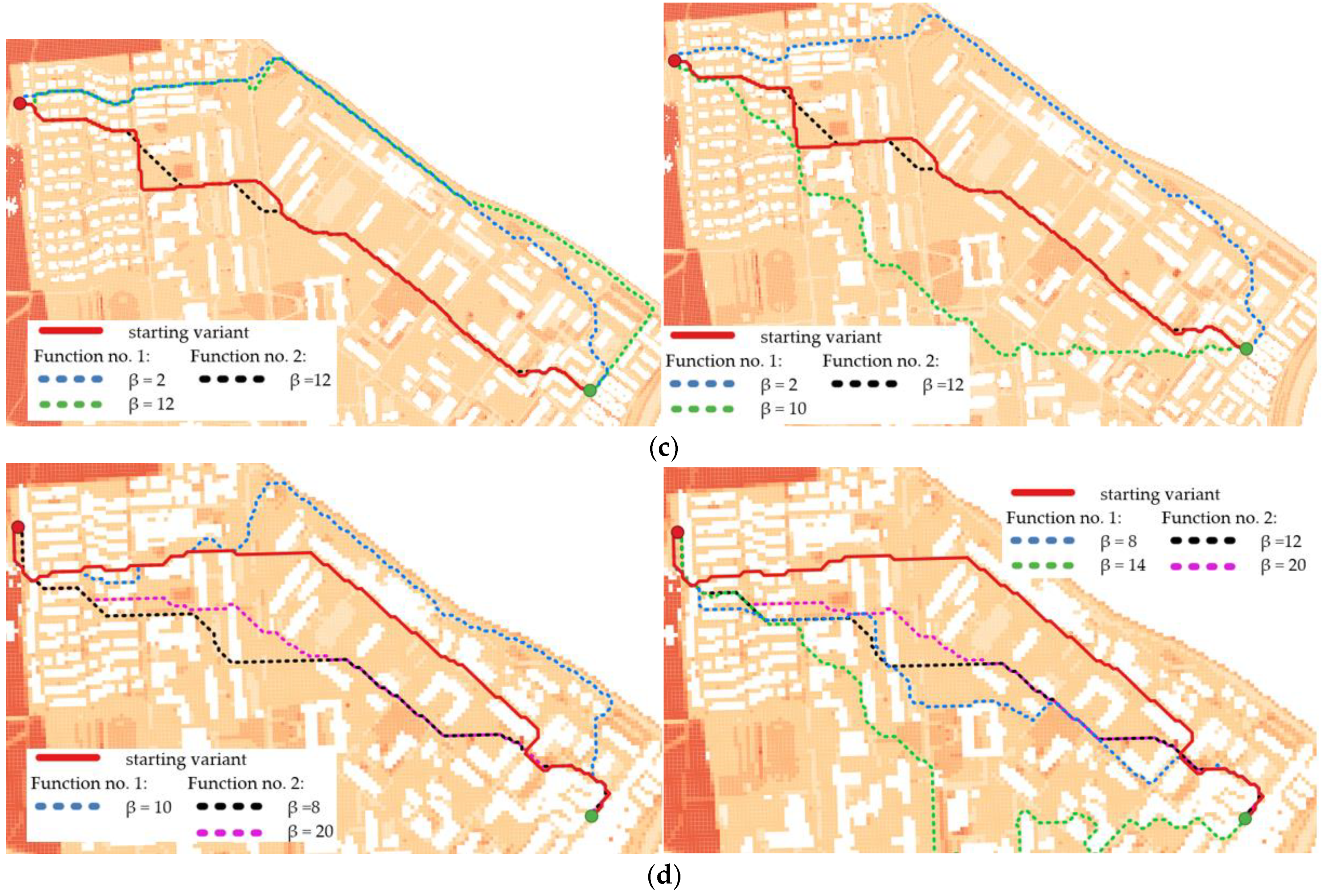
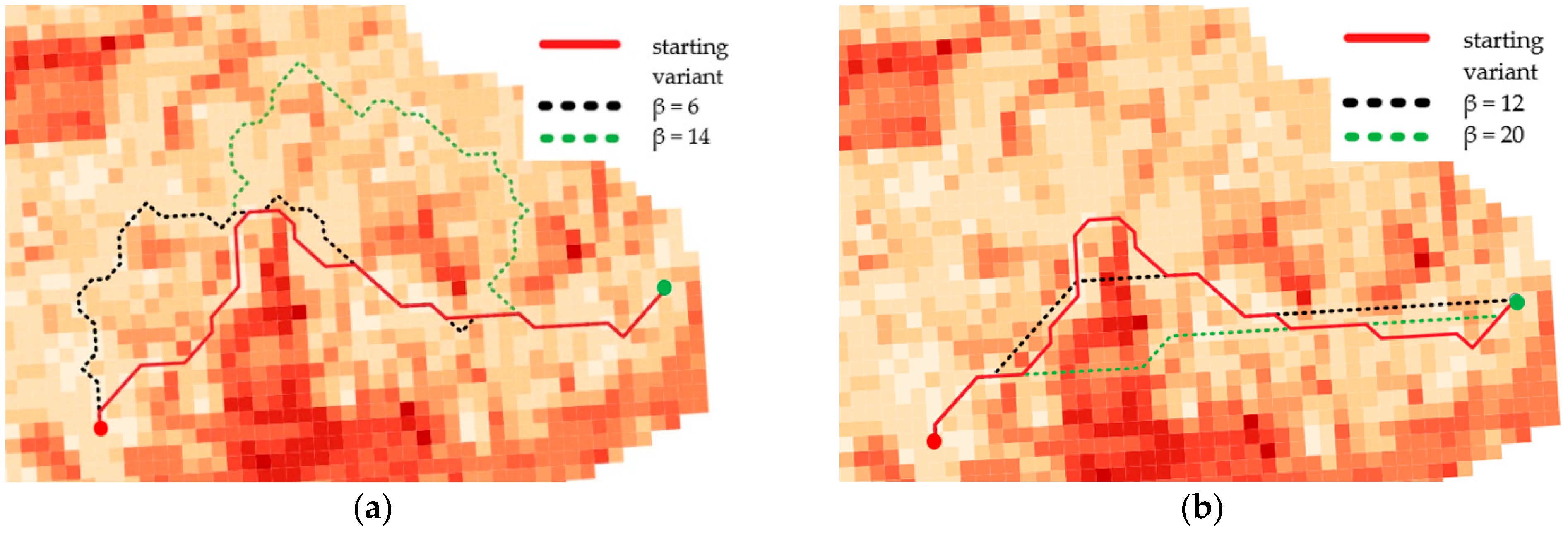
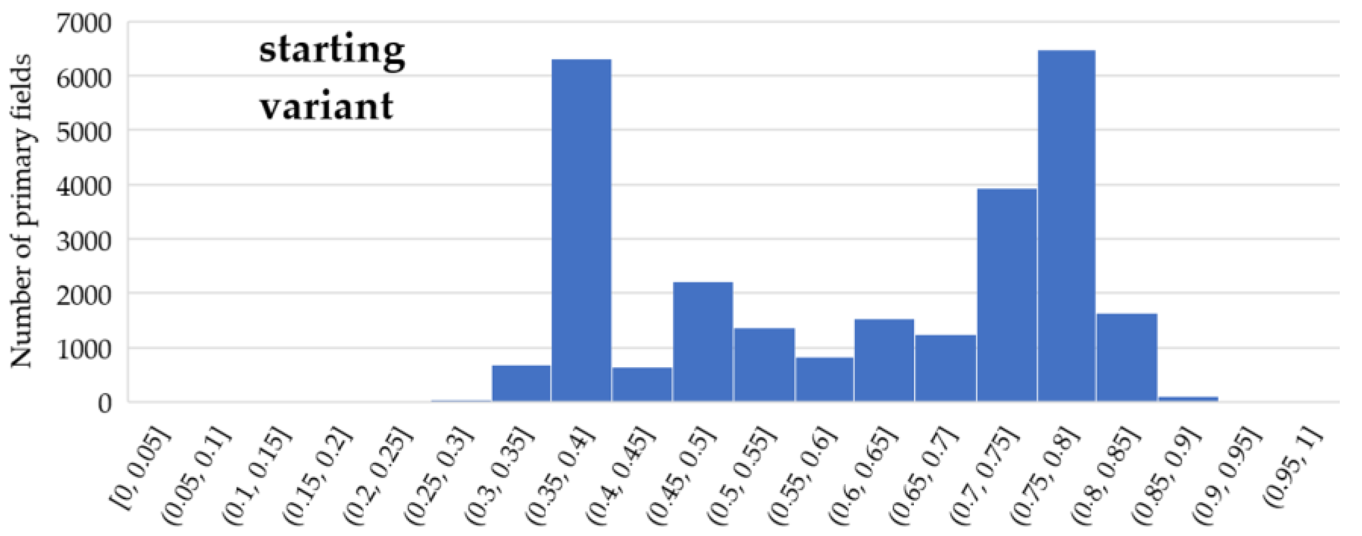
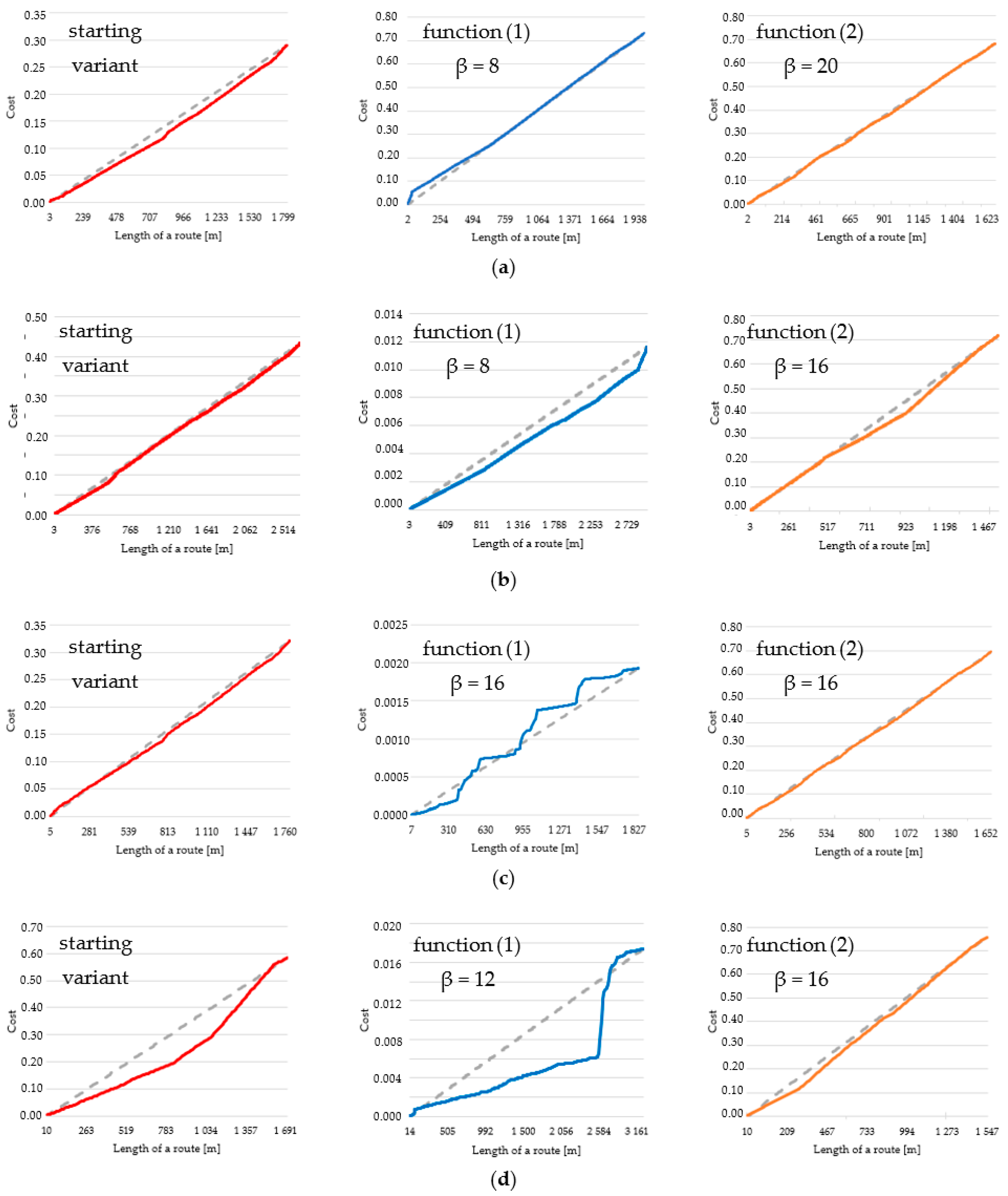
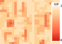
- Finding the route directly from the computed IOP values. This variant may be called a starting variant because the index values are not modified before determining the route. This variant is presented below in Figure 4.
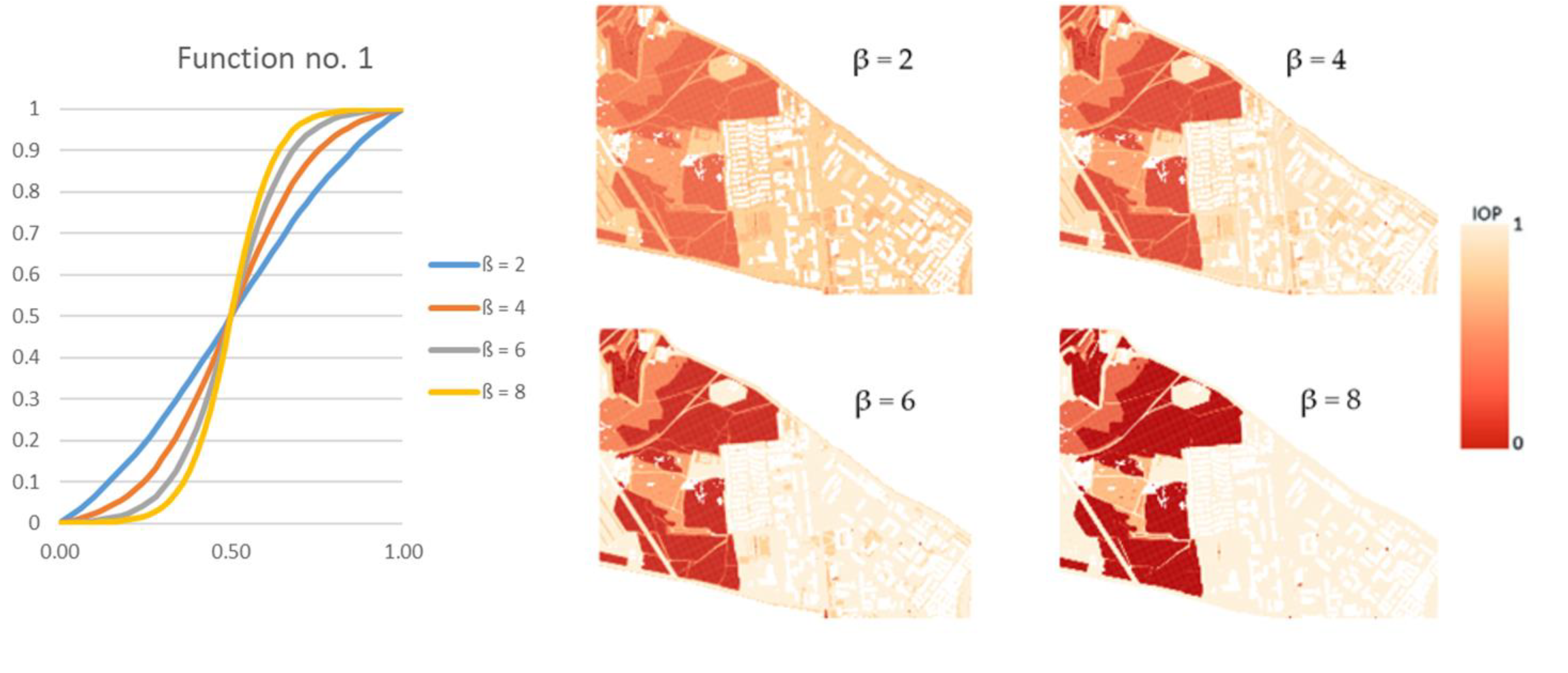
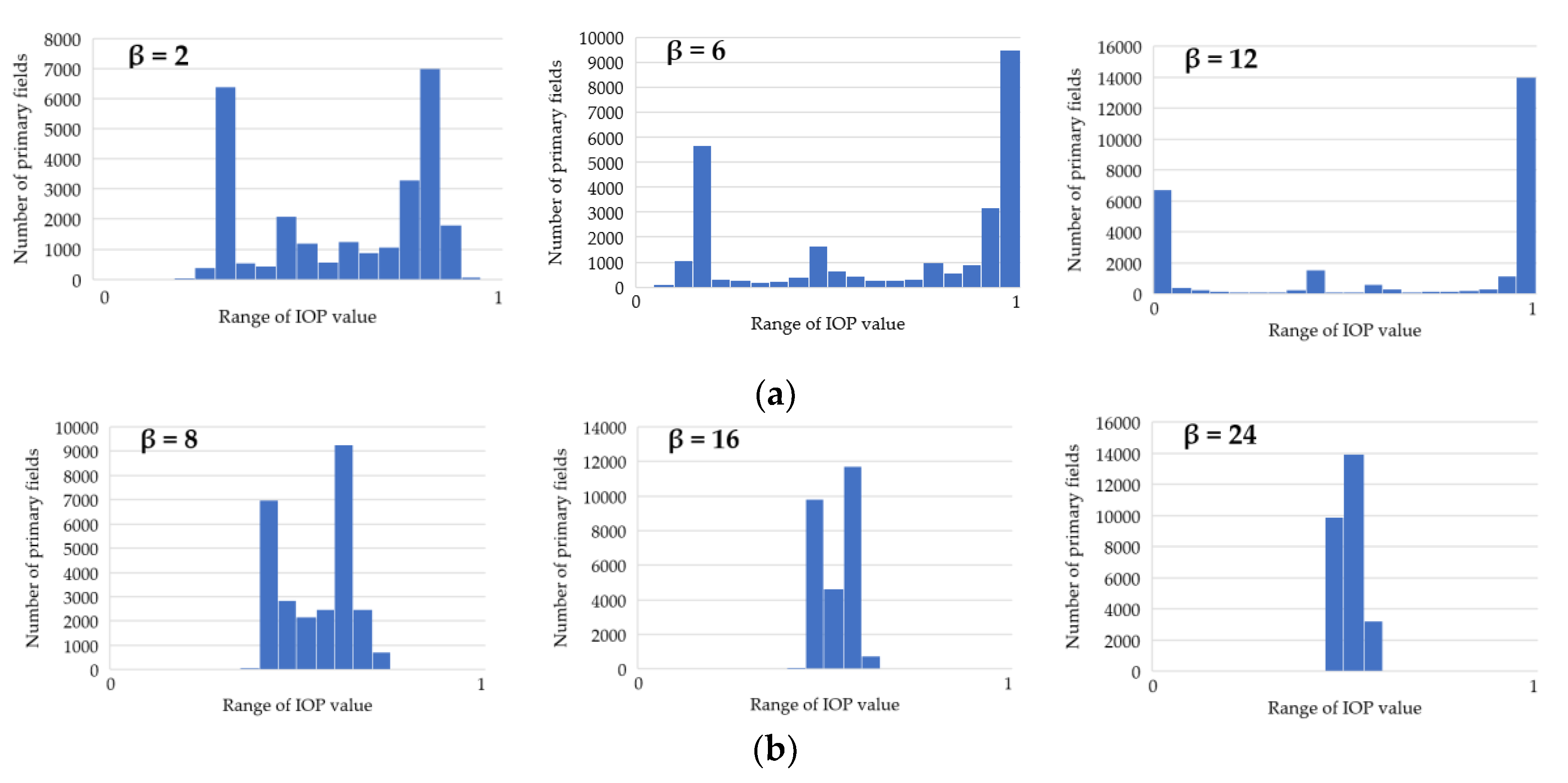
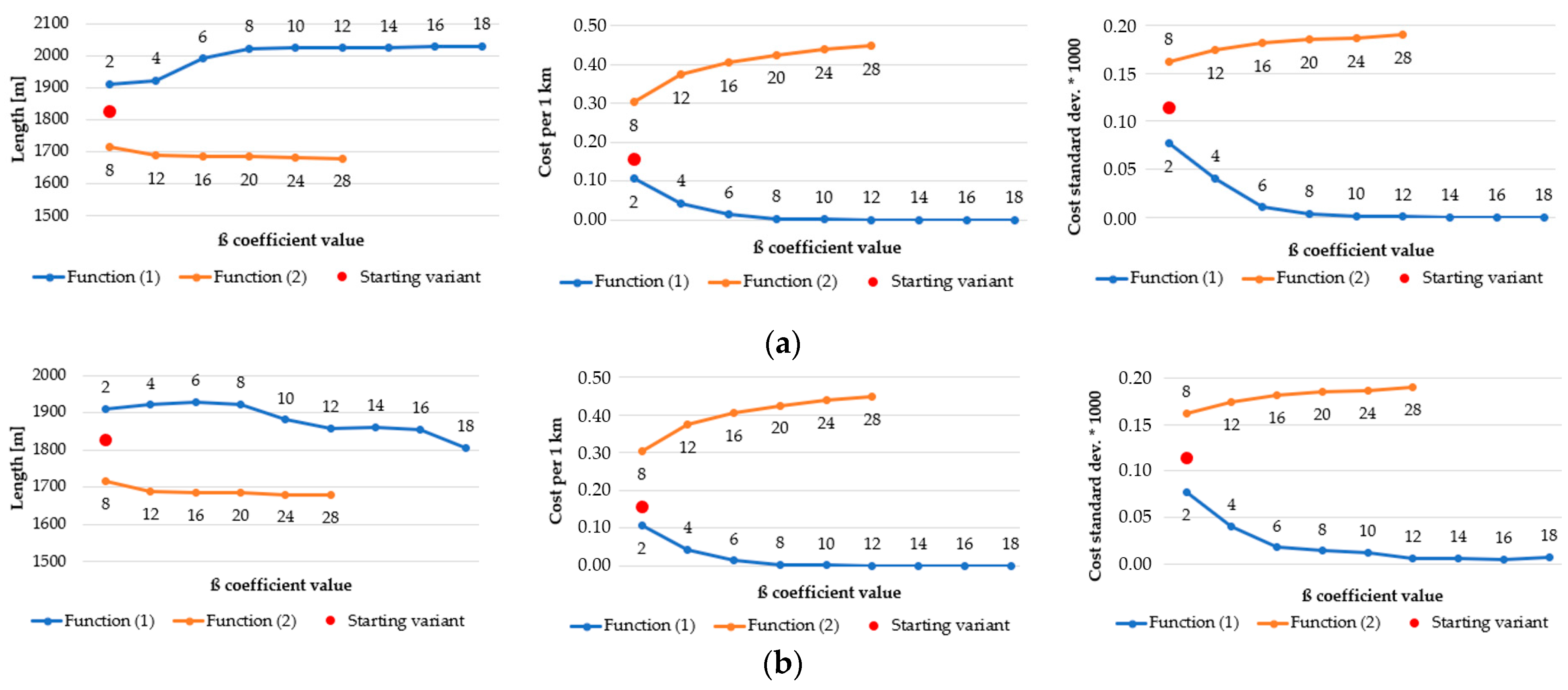
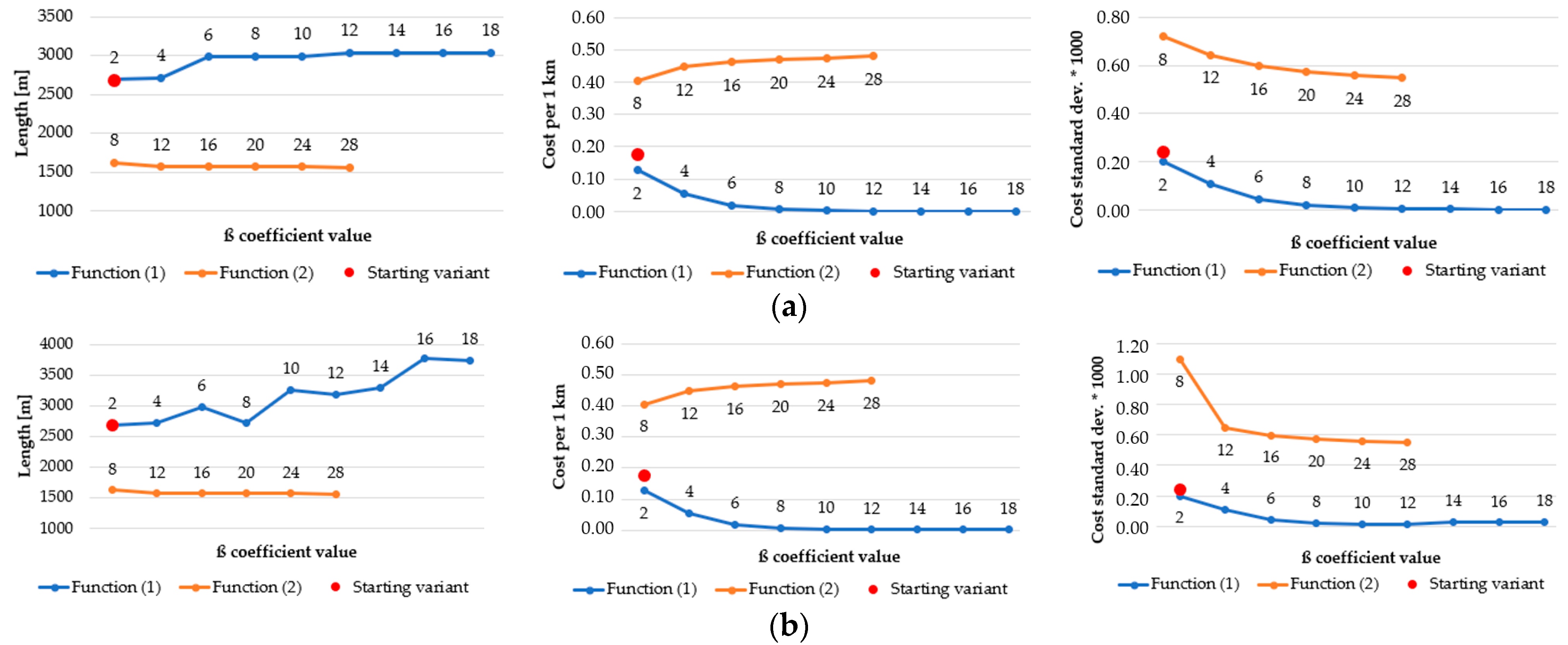
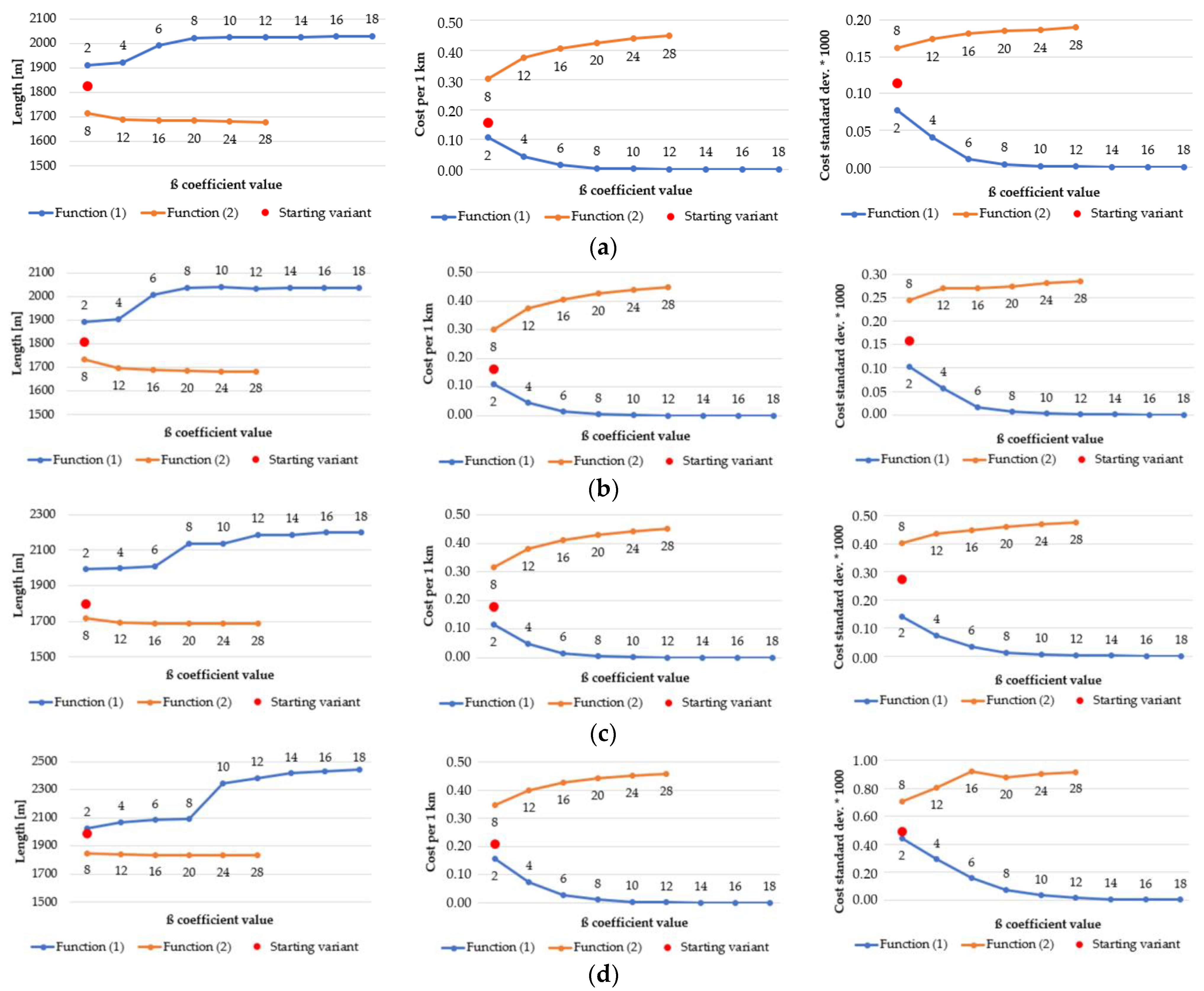
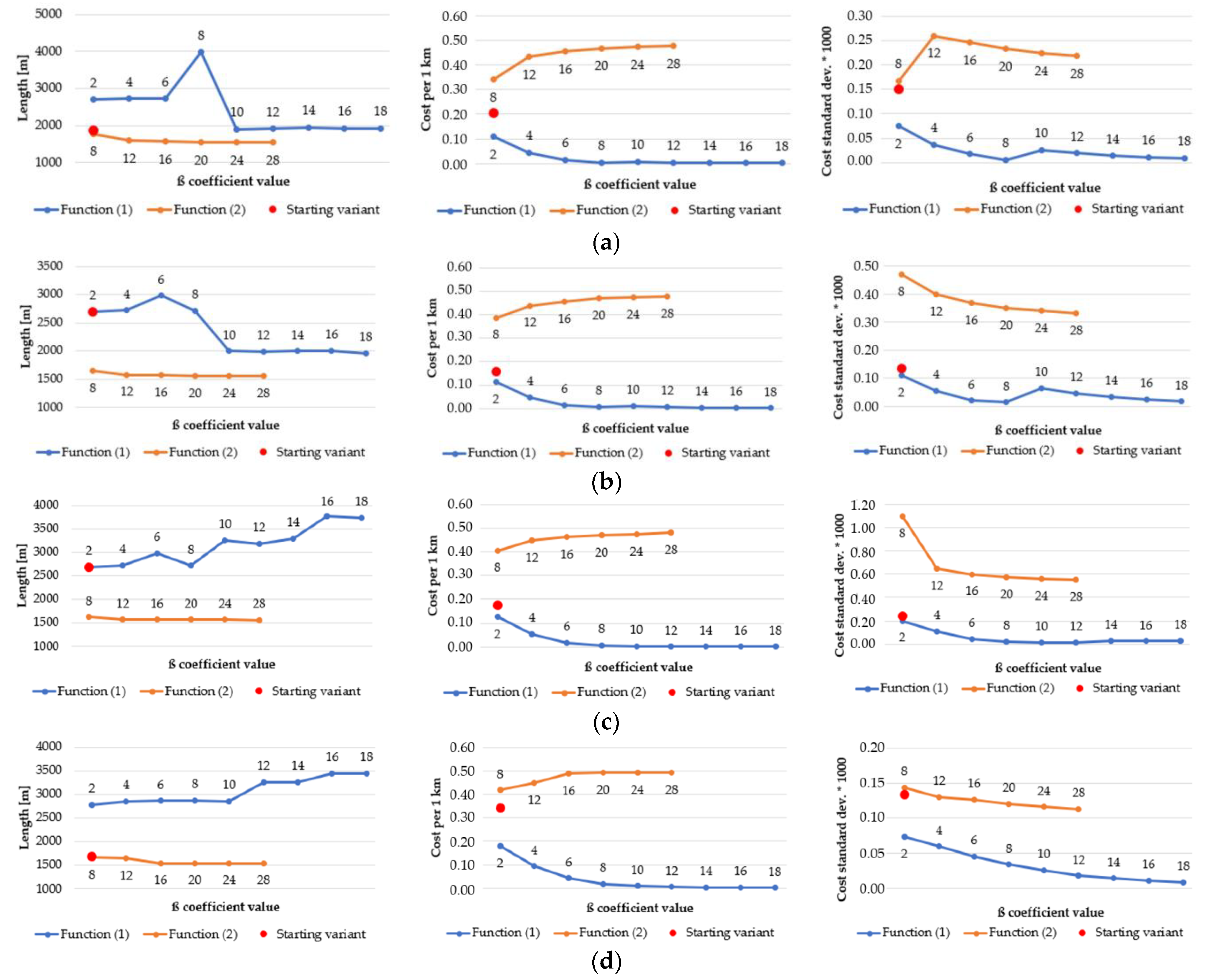
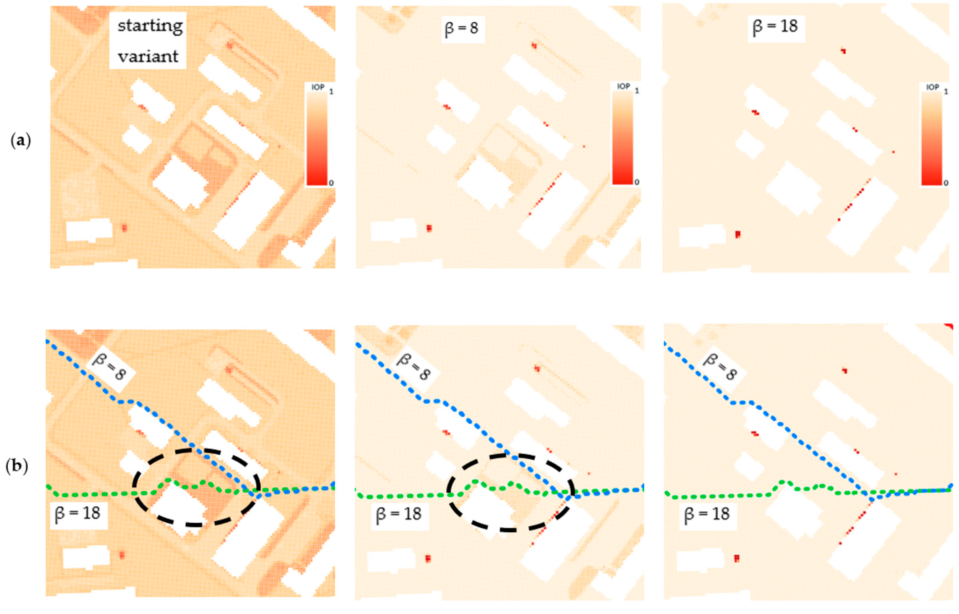
- Finding the route for modified IOP values by means of determining their new values with use of the following equation:where β is a coefficient that amplifies or weakens the impact of the function on the IOP value, e is the Euler’s number (e ≈ 2.71) and IOP is an original IOP value. Tests were performed for a β parameter ranging from 2 to 18 because lower or greater values did not significantly change the new IOPs. The use of Equation (1) allowed us to augment the differences between impassable and passable areas, which are visualized in Figure 5. This variant enables to determine a route that goes through an easy to overcome terrain and in most cases, it is longer than the route in the starting variant.
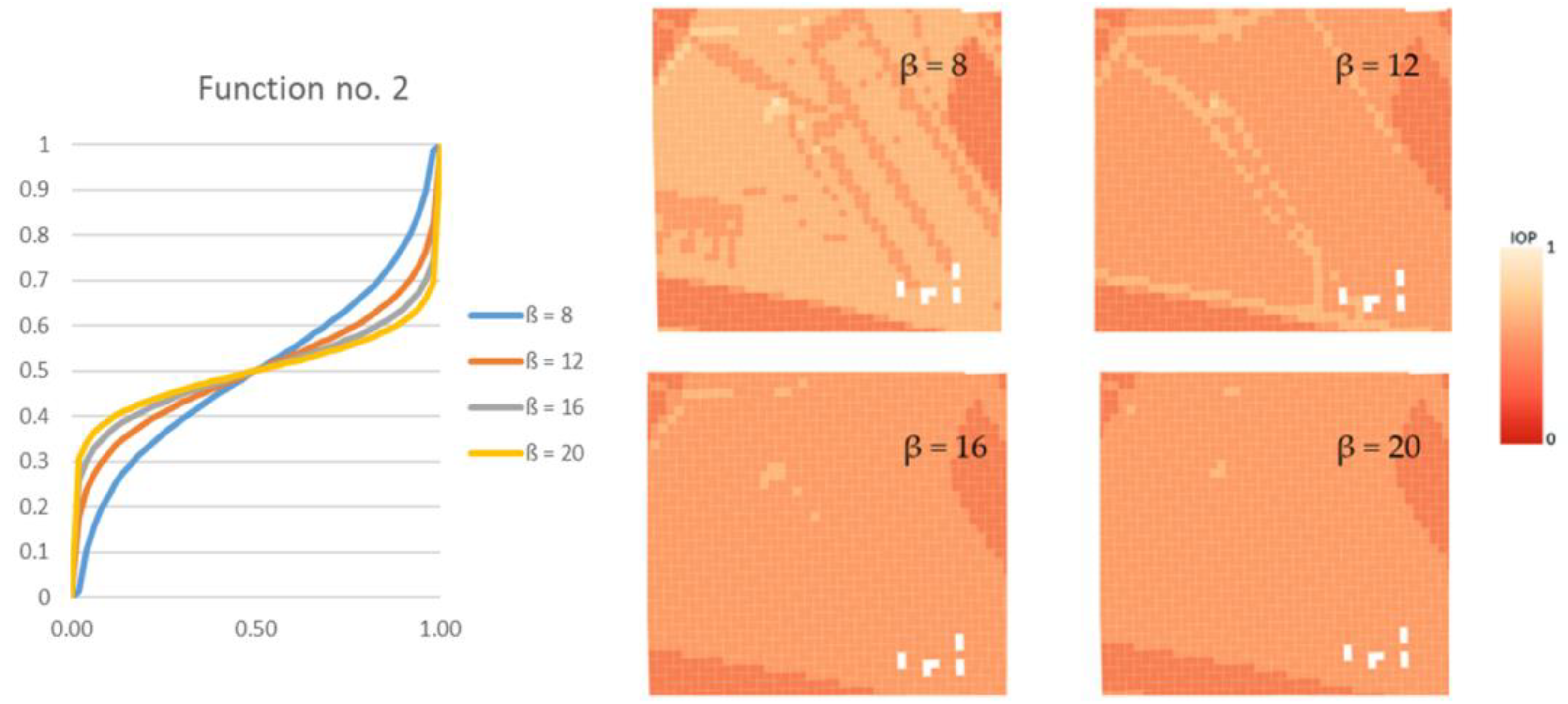
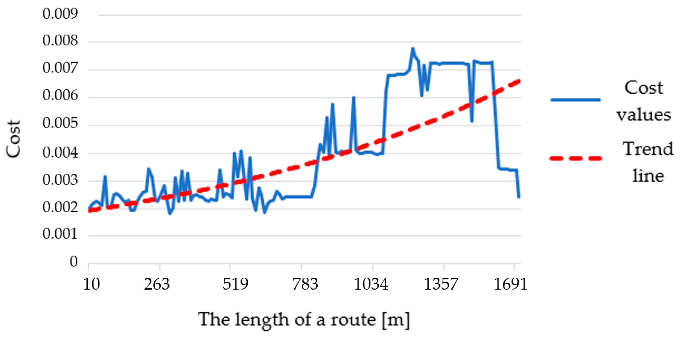
- Finding the route for modified IOP values by determination of their new values with use of the following equation:where ln marks the natural logarithm, IOP is an original IOP value, and the β parameter in this equation ranged from 2 to 24. Other values, similarly to the first function, did not significantly change the new IOPs. Thanks to this function, the IOPs distribution was flattened with a simultaneous decrease in the differences between passability indexes, which is presented in Figure 6. This solution enables to obtain a route which is significantly shorter but is leading through less passable areas.
2.2.4. Block No. 3
2.2.5. Block No. 5
2.2.6. Block No. 6
2.2.7. Block No. 7
2.2.8. Block No. 8
3. Results
- Model: DELL T640;
- Processor: 2 × Intel Xeon Gold 6230, 2.10 GHz;
- RAM: 64 GB;
- HDD: 4 × 1 TB SDD, RAID 5.
4. Discussion
5. Conclusions
Author Contributions
Funding
Conflicts of Interest
References
- Doyle, P.; Bennett, M.R. Military Geography: The Influence of Terrain in the Outcome of the Gallipoli Campaign, 1915. Geogr. J. 1999, 165, 12–36. [Google Scholar] [CrossRef]
- Maio, C.V.; Tenenbaum, D.E.; Brown, C.J.; Mastone, V.T.; Gontz, A.M. Application of Geographic Information Technologies to Historical Landscape Reconstruction and Military Terrain Analysis of an American Revolution Battlefield: Preservation Potential of Historic Lands in Urbanized Settings, Boston, Massachusetts, USA. J. Cult. Herit. 2013, 14, 317–331. [Google Scholar] [CrossRef]
- Department of the Army. Army Field Manual No. 5-33: Terrain Analysis; Department of the Army: Washington DC, USA, 1990. [Google Scholar]
- STANAG 3992: Military Geographic Documentation—Terrain Analysis-AGeoP-1 (A). 1999. Available online: https://standards.globalspec.com/std/464406/STANAG%203992 (accessed on 6 July 2021).
- Ministry of National Defence. Defence Standard NO-06-A015:2012. Terrain—Rules of Classification—Terrain Analysis on Operational Level; Ministry of National Defence of Poland: Krakow, Poland, 2012. [Google Scholar]
- Hubacek, M.; Ceplova, L.; Brenova, M.; Mikita, T.; Zerzan, P. Analysis of Vehicle Movement Possibilities in Terrain Covered by Vegetation. In Proceedings of the International Conference on Military Technologies (ICMT), Brno, Czech Republic, 19–21 May 2015; IEEE: Piscataway, NJ, USA, 2015; pp. 1–5. [Google Scholar]
- Rybansky, M. Trafficability Analysis through Vegetation. In Proceedings of the 2017 International Conference on Military Technologies (ICMT), Brno, Czech Republic, 31 May–2 June 2017; pp. 207–210. [Google Scholar]
- Rybansky, M. Determination the Ability of Military Vehicles to Override Vegetation. J. Terramech. 2020, 91, 129–138. [Google Scholar] [CrossRef]
- Hubáček, M.; Rybansky, M.; Cibulova, K.; Brenov, M.; Ceplova, L. Mapping the Passability of Soils for Vehicle Movement. Kvüõa Toim. 2015, 21, 5–18. [Google Scholar]
- Jayakumar, P.; Mechergui, D.; Wasfy, T.M. Understanding the Effects of Soil Characteristics on Mobility. In Proceedings of the ASME 2017 International Design Engineering Technical Conferences and Computers and Information in Engineering Conference, Cleveland, OH, USA, 6–9 August 2017. [Google Scholar] [CrossRef]
- Rybansky, M. Soil Trafficability Analysis. In Proceedings of the International Conference on Military Technologies (ICMT) 2015, Brno, Czech Republic, 19–21 May 2015; pp. 1–5. [Google Scholar]
- Hubáček, M.; Almášiová, L.; Dejmal, K.; Mertová, E. Combining Different Data Types for Evaluation of the Soils Passability. In The Rise of Big Spatial Data; Ivan, I., Singleton, A., Horák, J., Inspektor, T., Eds.; Springer International Publishing: Cham, Switzerland, 2017; pp. 69–84. [Google Scholar]
- Rybansky, M. Effect of the Geographic Factors on the Cross Country Movement during Military Operations and the Natural Disasters; University of Defence Brno: Brno, Czech Republic, 2007; ISBN 978-80-7231-238-2. [Google Scholar]
- Rybansky, M.; Hofmann, A.; Hubacek, M.; Kovarik, V.; Talhofer, V. The Impact of Terrain on Cross-Country Mobility—Geographic Factors and Their Characteristics. In Proceedings of the 18th International Conference of the ISTVS, Seoul, Korea, 22–25 September 2014; ISBN 978-1-942112-45-7. [Google Scholar]
- Hošková-Mayerová, Š.; Talhofer, V.; Otřísal, P.; Rybanský, M. Influence of Weights of Geographical Factors on the Results of Multicriteria Analysis in Solving Spatial Analyses. ISPRS Int. J. Geo Inf. 2020, 9, 489. [Google Scholar] [CrossRef]
- McCullough, M.; Jayakumar, P.; Dasch, J.; Gorsich, D. The Next Generation NATO Reference Mobility Model Development. J. Terramech. 2017, 73, 49–60. [Google Scholar] [CrossRef]
- Paramsothy, J.; Bradbury, M.; Dasch, J.; Gonzalez, R.; Hodges, H.; Jain, A.; Iagnemma, K.; Letherwood, M.; McCullough, M.; Priddy, J.; et al. Next-Generation NATO Reference Mobility Model (NRMM) Development; Defense Technical Information Center: Fort Belvoir, VA, USA, 2018. [Google Scholar]
- Wasfy, T.; Jayakumar, P. Next-Generation NATO Reference Mobility Model Complex Terramechanics—Part 1: Definition and Literature Review. J. Terramech. 2021. [Google Scholar] [CrossRef]
- Gonzalez, R.; Jayakumar, P.; Iagnemma, K. An Efficient Method for Increasing the Accuracy of Mobility Maps for Ground Vehicles. J. Terramech. 2016, 68, 23–35. [Google Scholar] [CrossRef]
- Maclaurin, B. Comparing the NRMM (VCI), MMP and VLCI Traction Models. J. Terramech. 2007, 44, 43–51. [Google Scholar] [CrossRef]
- Shoop, S.; Knuth, M.; Wieder, W. Measuring Vehicle Impacts on Snow Roads. J. Terramech. 2013, 50, 63–71. [Google Scholar] [CrossRef]
- Pokonieczny, K. Automatic Military Passability Map Generation System. In Proceedings of the 2017 International Conference on Military Technologies (ICMT), Brno, Czech Republic, 31 May–2 June 2017; IEEE: Piscataway, NJ, USA, 2017; pp. 285–292. [Google Scholar]
- Pokonieczny, K. Comparison of Land Passability Maps Created with Use of Different Spatial Data Bases. Geogr. Sb. CGS 2018, 123, 317–352. [Google Scholar] [CrossRef]
- Pokonieczny, K.; Mościcka, A. The Influence of the Shape and Size of the Cell on Developing Military Passability Maps. ISPRS Int. J. Geo-Inf. 2018, 7, 261. [Google Scholar] [CrossRef] [Green Version]
- Pokonieczny, K. The Methodology of Creating Variable Resolution Maps Based on the Example of Passability Maps. ISPRS Int. J. Geo-Inf. 2020, 9, 738. [Google Scholar] [CrossRef]
- Pokonieczny, K. Methodology of Cartographic Visualisation of Military Maps of Passability. In Proceedings of the 7th International Conference on Cartography & GIS, Sozopol, Bulgaria, 18 June 2018; pp. 613–622. [Google Scholar]
- Pokonieczny, K. Use of a Multilayer Perceptron to Automate Terrain Assessment for the Needs of the Armed Forces. ISPRS Int. J. Geo-Inf. 2018, 7, 430. [Google Scholar] [CrossRef] [Green Version]
- Pokonieczny, K. Methods of Using Self-Organising Maps for Terrain Classification, Using an Example of Developing a Military Passability Map. In Proceedings of the Conference GIS Ostrava, Ostrava, Czech Republic, 22–24 March 2017; Springer: Cham, Switzerland, 2017; pp. 359–371. [Google Scholar]
- Dawid, W.; Pokonieczny, K. Analysis of the Possibilities of Using Different Resolution Digital Elevation Models in the Study of Microrelief on the Example of Terrain Passability. Remote Sens. 2020, 12, 4146. [Google Scholar] [CrossRef]
- Pokonieczny, K.; Borkowska, S. Using High Resolution Spatial Data to Develop Military Maps of Passability. In Proceedings of the 2019 International Conference on Military Technologies (ICMT), Brno, Czech Republic, 30–31 May 2019; pp. 1–8. [Google Scholar]
- Kapi, A.Y.; Sunar, M.S.; Algfoor, Z.A. Summary of Pathfinding in Off-Road Environment. In Proceedings of the 2020 6th International Conference on Interactive Digital Media (ICIDM), Virtual Conference, Bandung, Indonesia, 14–15 December 2020; pp. 1–4. [Google Scholar]
- Campbell, S.; O’Mahony, N.; Carvalho, A.; Krpalkova, L.; Riordan, D.; Walsh, J. Path Planning Techniques for Mobile Robots A Review. In Proceedings of the 2020 6th International Conference on Mechatronics and Robotics Engineering (ICMRE), Barcelona, Spain, 12–15 February 2020; pp. 12–16. [Google Scholar]
- Borges, C.D.B.; Almeida, A.M.A.; Paula Júnior, I.C.; de Mesquita Sá Junior, J.J. A Strategy and Evaluation Method for Ground Global Path Planning Based on Aerial Images. Expert Syst. Appl. 2019, 137, 232–252. [Google Scholar] [CrossRef]
- Graf, U.; Borges, P.; Hernández, E.; Siegwart, R.; Dubé, R. Optimization-Based Terrain Analysis and Path Planning in Unstructured Environments. In Proceedings of the 2019 International Conference on Robotics and Automation (ICRA), Montreal, QC, Canada, 20–24 May 2019; pp. 5614–5620. [Google Scholar]
- Ng, M.-K.; Chong, Y.-W.; Ko, K.; Park, Y.-H.; Leau, Y.-B. Adaptive Path Finding Algorithm in Dynamic Environment for Warehouse Robot. Neural Comput. Applic. 2020, 32, 13155–13171. [Google Scholar] [CrossRef]
- Wei, C.; Ni, F. Multiobjective Model-Free Learning for Robot Pathfinding with Environmental Disturbances. Int. J. Adv. Robot. Syst. 2019, 16, 1729881419885703. [Google Scholar] [CrossRef]
- Jiang, L.; Zhao, P.; Dong, W.; Li, J.; Ai, M.; Wu, X.; Hu, Q. An Eight-Direction Scanning Detection Algorithm for the Mapping Robot Pathfinding in Unknown Indoor Environment. Sensors 2018, 18, 4254. [Google Scholar] [CrossRef] [PubMed] [Green Version]
- Abd Algfoor, Z.; Sunar, M.S.; Kolivand, H. A Comprehensive Study on Pathfinding Techniques for Robotics and Video Games. Int. J. Comput. Games Technol. 2015, 2015, e736138. [Google Scholar] [CrossRef]
- Ropero, F.; Muñoz, P.; R-Moreno, M.D. TERRA: A Path Planning Algorithm for Cooperative UGV–UAV Exploration. Eng. Appl. Artif. Intell. 2019, 78, 260–272. [Google Scholar] [CrossRef]
- Mocholi, J.A.; Jaen, J.; Catala, A.; Navarro, E. An Emotionally Biased Ant Colony Algorithm for Pathfinding in Games. Expert Syst. Appl. 2010, 37, 4921–4927. [Google Scholar] [CrossRef]
- Shan, Y. Study on Submarine Path Planning Based on Modified Ant Colony Optimization Algorithm. In Proceedings of the 2018 IEEE International Conference on Mechatronics and Automation (ICMA), Changchun, China, 5–8 August 2018; pp. 288–292. [Google Scholar]
- Wang, H.; Zhang, H.; Wang, K.; Zhang, C.; Yin, C.; Kang, X. Off-Road Path Planning Based on Improved Ant Colony Algorithm. Wirel. Pers. Commun. 2018, 102, 1705–1721. [Google Scholar] [CrossRef]
- Mora, A.M.; Merelo, J.J.; Millán, C.; Torrecillas, J.; Laredo, J.L.J.; Castillo, P.A. Comparing ACO Algorithms for Solving the Bi-Criteria Military Path-Finding Problem. In Advances in Artificial Life; Almeida e Costa, F., Rocha, L.M., Costa, E., Harvey, I., Coutinho, A., Eds.; Springer: Berlin/Heidelberg, Germany, 2007; pp. 665–674. [Google Scholar]
- Raja, R.; Dutta, A. Path Planning in Dynamic Environment for a Rover Using A∗ and Potential Field Method. In Proceedings of the 2017 18th International Conference on Advanced Robotics (ICAR), Hong Kong, China, 10–12 July 2017; pp. 578–582. [Google Scholar]
- Muñoz, P.; R-Moreno, M.D.; Castaño, B. 3Dana: A Path Planning Algorithm for Surface Robotics. Eng. Appl. Artif. Intell. 2017, 60, 175–192. [Google Scholar] [CrossRef]
- Fujimura, K.; Samet, H. A Hierarchical Strategy for Path Planning among Moving Obstacles (Mobile Robot). IEEE Trans. Robot. Autom. 1989, 5, 61–69. [Google Scholar] [CrossRef]
- Liu, Q.; Zhao, L.; Tan, Z.; Chen, W. Global Path Planning for Autonomous Vehicles in Off-Road Environment via an A-Star Algorithm. Int. J. Veh. Auton. Syst. 2017, 13, 330–339. [Google Scholar] [CrossRef]
- Choi, S.; Park, J.; Lim, E.; Yu, W. Global Path Planning on Uneven Elevation Maps. In Proceedings of the 2012 9th International Conference on Ubiquitous Robots and Ambient Intelligence (URAI), Daejeon, Korea, 26–28 November 2012; pp. 49–54. [Google Scholar]
- Ganganath, N.; Cheng, C.-T.; Tse, C.K. Finding Energy-Efficient Paths on Uneven Terrains. In Proceedings of the 2014 10th France-Japan/8th Europe-Asia Congress on Mecatronics (MECATRONICS2014—Tokyo), Tokyo, Japan, 27–29 November 2014; pp. 383–388. [Google Scholar]
- Saranya, C.; Unnikrishnan, M.; Ali, S.A.; Sheela, D.S.; Lalithambika, V.R. Terrain Based D∗ Algorithm for Path Planning. IFAC Pap. Online 2016, 49, 178–182. [Google Scholar] [CrossRef]
- García, A.M.; Guervós, J.J.M.; Laredo, J.L.; Valdivieso, P.; Millán, C.; Torrecillas, J. Balancing Safety and Speed in the Military Path Finding Problem: Analysis of Different ACO Algorithms. In Proceedings of the 9th Annual Conference Companion on Genetic and Evolutionary Computation, London, UK, 7–11 July 2007. [Google Scholar]
- Leenen, L.; Terlunen, A. A Focussed Dynamic Path Finding Algorithm with Constraints. In Proceedings of the 2013 International Conference on Adaptive Science and Technology, Pretoria, South Africa, 25–27 November 2013; pp. 1–8. [Google Scholar]
- Leenen, L.; Terlunen, A.; le Roux, H. A Constraint Programming Solution for the Military Unit Path Finding Problem; Taylor & Francis Group: Boca Raton, FL, USA, 2012; ISBN 978-0-429-10481-7. [Google Scholar]
- Leenen, L.; Vorster, J.; le Roux, H. A Constraint-Based Solver for the Military Unit Path Finding Problem. In Proceedings of the 2010 Spring Simulation Multiconference, Orlando, FL, USA, 11–15 April 2010; Society for Computer Simulation International: San Diego, CA, USA, 2010; pp. 1–8. [Google Scholar]
- Duc, L.M.; Sidhu, A.S.; Chaudhari, N.S. Hierarchical Pathfinding and AI-Based Learning Approach in Strategy Game Design. Int. J. Comput. Games Technol. 2008, 2008, e873913. [Google Scholar] [CrossRef] [Green Version]
- John, T.C.H.; Prakash, E.C.; Chaudhari, N.S. Strategic Team AI Path Plans: Probabilistic Pathfinding. Int. J. Comput. Games Technol. 2008, 2008, e834616. [Google Scholar] [CrossRef] [Green Version]
- Tarapata, Z. Military Route Planning in Battlefield Simulation: Effectiveness Problems and Potential Solutions. J. Telecommun. Inf. Technol. 2003, 4, 47–56. [Google Scholar]
- Kamphuis, A.; Rook, M.; Overmars, M.H. Tactical Path Finding in Urban Environments. In Proceedings of the First International Workshop on Crowd Simulation, Lausanne, Switzerland, 24–25 November 2005. [Google Scholar]
- Foead, D.; Ghifari, A.; Kusuma, M.B.; Hanafiah, N.; Gunawan, E. A Systematic Literature Review of A* Pathfinding. Procedia Comput. Sci. 2021, 179, 507–514. [Google Scholar] [CrossRef]
- Schulz, F.; Wagner, D.; Weihe, K. Dijkstra’s Algorithm On-Line: An Empirical Case Study from Public Railroad Transport. Algorithm Eng. 1999, 110–123. [Google Scholar] [CrossRef]
- Pokonieczny, K.; Dawid, W. Methodology of Using Terrain Passability Maps for Planning the Movement of Troops and Navigation of Unmanned Ground Vehicles. In Proceedings of the Conference GIS Ostrava 2021 Advances in Localization and Navigation, Ostrava, Czech Republic, 17–19 March 2021; Vysoká Škola Báňská—Technická Univerzita: Ostrava, Czech Republic, 2021. [Google Scholar]
- National Imagery and Mapping Agency. Military Specification MIL-V-89032 Vector Smart Map (VMAP) Level 2; National Geospatial-Intelligence Agency: Fort Belvoir, VA, USA, 1993. [Google Scholar]
- Digital Geographic Information Standard (DIGEST), 2nd ed.; STANAG 7074; Department of US Army: Washington, DC, USA, 1998.
- Farr, T.G.; Rosen, P.A.; Caro, E.; Crippen, R.; Duren, R.; Hensley, S.; Kobrick, M.; Paller, M.; Rodriguez, E.; Roth, L.; et al. The Shuttle Radar Topography Mission. Rev. Geophys. 2007, 45, RG2004. [Google Scholar] [CrossRef] [Green Version]
- Fitro, A.; Bachri, O.S.; Purnomo, A.I.S.; Frendianata, I. Shortest Path Finding in Geographical Information Systems Using Node Combination and Dijkstra Algorithm. Int. J. Mech. Eng. Technol. 2018, 9, 755–760. [Google Scholar]
- Javaid, M.A. Understanding Dijkstra’s Algorithm. SSRN Electron. J. 2013, 28. [Google Scholar] [CrossRef]
- Cui, X.; Shi, H. A*-Based Pathfinding in Modern Computer Games. IJCSNS Int. J. Comput. Sci. Netw. Secur. 2011, 11, 7. [Google Scholar]
- Duchoň, F.; Babinec, A.; Kajan, M.; Beňo, P.; Florek, M.; Fico, T.; Jurišica, L. Path Planning with Modified a Star Algorithm for a Mobile Robot. Procedia Eng. 2014, 96, 59–69. [Google Scholar] [CrossRef] [Green Version]
- Dere, E.; Durdu, A. Usage of the A* Algorithm to Find the Shortest Path in Transportation Systems. In Proceedings of the International Conference on Advanced Technologies, Computer Engineering and Science (ICATCES’18), Safranbolu, Turkey, 11–13 May 2018; p. 4. [Google Scholar]

| Troop Size | Troop Symbol | Size of Primary Field | Width of an Avenue of Approach |
|---|---|---|---|
| Single vehicle |  | 2–5 m | 10 m |
| Team |  | 10 m | 20 m |
| Squad |  | 20 m | 50 m |
| Section |  | 50 m | 100 m |
| Platoon |  | 100 m | 200 m |
| Company |  | 200 m | 500 m |
| Battalion |  | 500 m | 1500 m |
| Brigade |  | 1000 m | 3000 m |
| Division |  | 2000 m | 6000 m |
| Corps |  | 5000 m | 15,000 m |
| 200 × 200 m | 1000 × 1000 m | 2000 × 2000 m |
 | 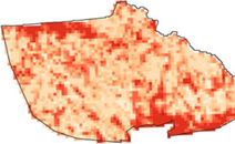 | 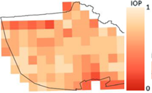 |
| 3 × 3 m | 10 × 10 m | 20 × 20 m |
 |  |  |
| Resolution | Generation Times | |||||
|---|---|---|---|---|---|---|
| Dijkstra’s Algorithm | A-Star Algorithm | |||||
| Route Determination | Export to SHP File | Total Time | Route Determination | Export to SHP File | Total Time | |
| 2 m | 7.46 s | 2 min 52.95 s | 3 min 0.41 s | 8.91 s | 2 min 48.74 s | 2 min 57.65 s |
| 3 m | 2.90 s | 1 min 14.40 s | 1 min 17.30 s | 3.57 s | 1 min 14.47 s | 1 min 18.04 s |
| 5 m | 0.86 s | 32.42 s | 33.28 s | 1.05 s | 32.88 s | 33.93 s |
| 10 m | 0.27 s | 4.56 s | 4.83 s | 0.34 s | 4.52 s | 4.86 s |
Publisher’s Note: MDPI stays neutral with regard to jurisdictional claims in published maps and institutional affiliations. |
© 2021 by the authors. Licensee MDPI, Basel, Switzerland. This article is an open access article distributed under the terms and conditions of the Creative Commons Attribution (CC BY) license (https://creativecommons.org/licenses/by/4.0/).
Share and Cite
Dawid, W.; Pokonieczny, K. Methodology of Using Terrain Passability Maps for Planning the Movement of Troops and Navigation of Unmanned Ground Vehicles. Sensors 2021, 21, 4682. https://doi.org/10.3390/s21144682
Dawid W, Pokonieczny K. Methodology of Using Terrain Passability Maps for Planning the Movement of Troops and Navigation of Unmanned Ground Vehicles. Sensors. 2021; 21(14):4682. https://doi.org/10.3390/s21144682
Chicago/Turabian StyleDawid, Wojciech, and Krzysztof Pokonieczny. 2021. "Methodology of Using Terrain Passability Maps for Planning the Movement of Troops and Navigation of Unmanned Ground Vehicles" Sensors 21, no. 14: 4682. https://doi.org/10.3390/s21144682
APA StyleDawid, W., & Pokonieczny, K. (2021). Methodology of Using Terrain Passability Maps for Planning the Movement of Troops and Navigation of Unmanned Ground Vehicles. Sensors, 21(14), 4682. https://doi.org/10.3390/s21144682