
General Purpose Low-Level Reinforcement Learning Control for Multi-Axis Rotor Aerial Vehicles †


Abstract
:1. Introduction
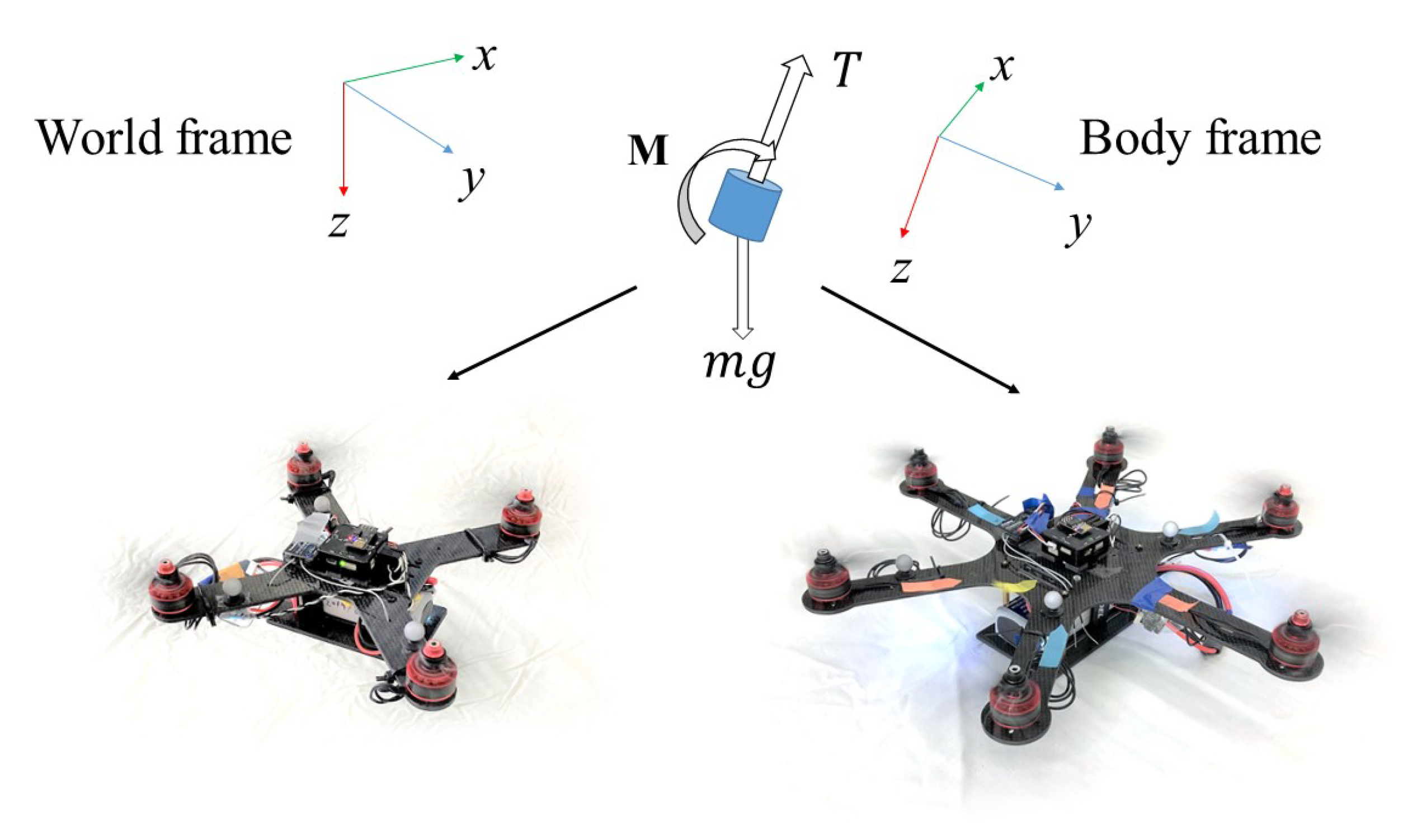
2. Background
3. Reinforcement Learning Algorithm and Implementation
3.1. Algorithm
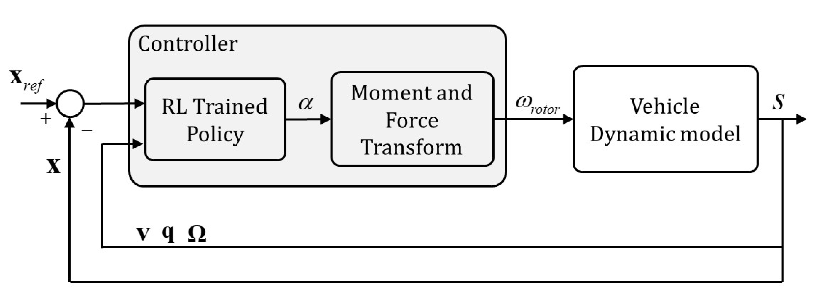
3.2. Implementation
| Algorithm 1 Learning Algorithm |
|
4. Experiments and Verification
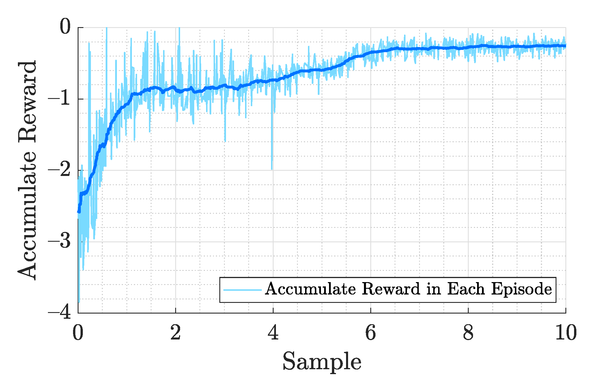
4.1. Reinforcement Learning Training
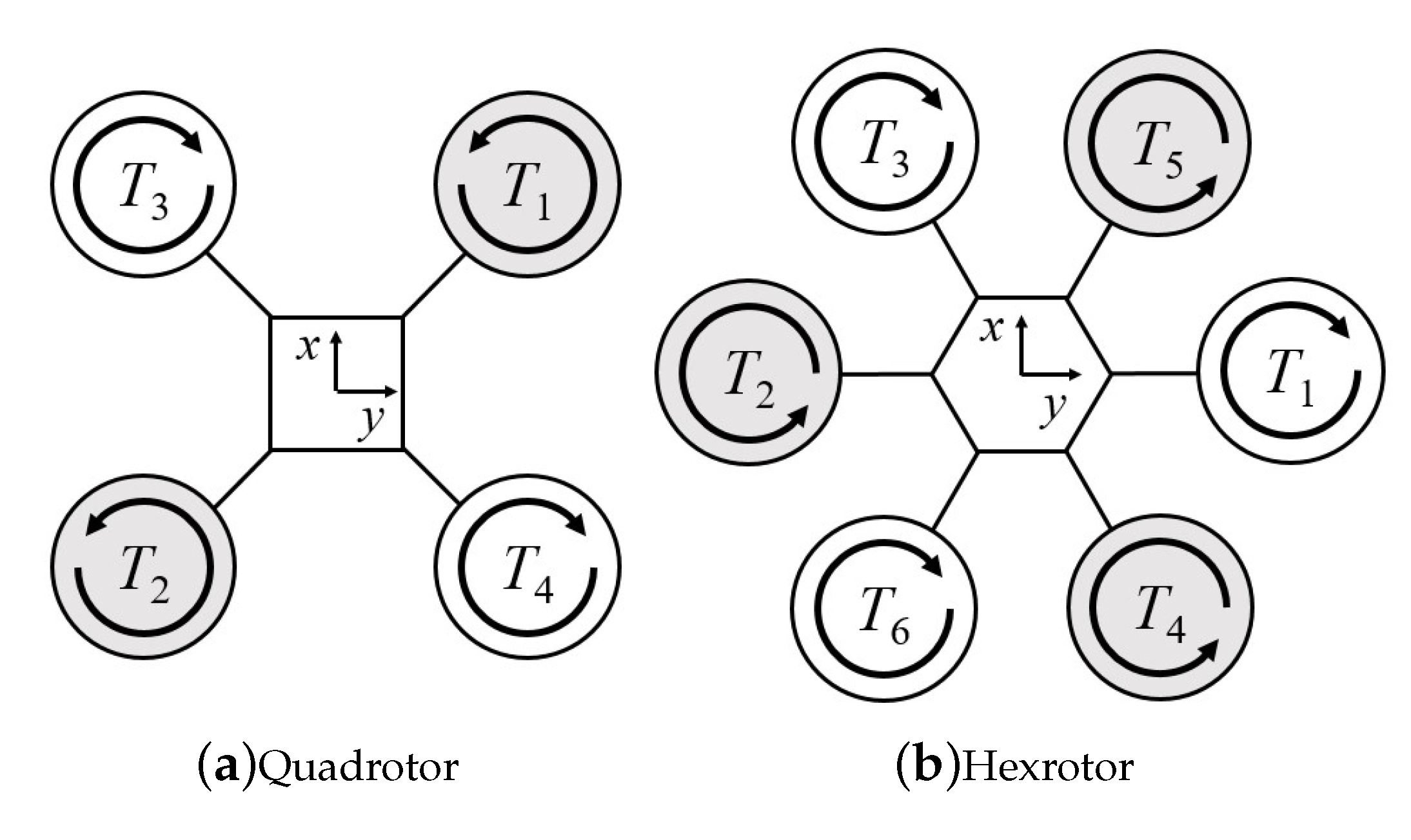
4.2. Mapping Strategy
4.3. Simulation Verification
4.4. Real-World Verification
5. Conclusions
Author Contributions
Funding
Institutional Review Board Statement
Informed Consent Statement
Data Availability Statement
Conflicts of Interest
References
- Duc, M.; Trong, T.N.; Xuan, Y.S. The quadrotor MAV system using PID control. In Proceedings of the 2015 IEEE International Conference on Mechatronics and Automation (ICMA), Beijing, China, 2–5 August 2015; pp. 506–510. [Google Scholar]
- Khatoon, S.; Gupta, D.; Das, L. PID & LQR control for a quadrotor: Modeling and simulation. In Proceedings of the 2014 International Conference on Advances in Computing, Communications and Informatics (ICACCI), Delhi, India, 24–27 September 2014; pp. 796–802. [Google Scholar]
- Bouabdallah, S.; Noth, A.; Siegwart, R. PID vs. LQ control techniques applied to an indoor micro quadrotor. In Proceedings of the 2004 IEEE/RSJ International Conference on Intelligent Robots and Systems (IROS) (IEEE Cat. No.04CH37566), Sendai, Japan, 28 September–2 October 2004; Volume 3, pp. 2451–2456. [Google Scholar]
- Bouabdallah, S.; Siegwart, R. Full control of a quadrotor. In Proceedings of the 2007 IEEE/RSJ International Conference on Intelligent Robots and Systems, San Diego, CA, USA, 29 October–2 November 2007; pp. 153–158. [Google Scholar]
- Mahony, R.E.; Kumar, V.; Corke, P.I. Multirotor Aerial Vehicles: Modeling, Estimation, and Control of Quadrotor. IEEE Robot. Autom. Mag. 2012, 19, 20–32. [Google Scholar] [CrossRef]
- Homann, G.M.; Huang, H.; Waslander, S.L.; Tomlin, C.J. Quadrotor Helicopter Flight Dynamics and Control: Theory and Experiment. In Proceedings of the AIAA Guidance, Navigation and Control Conference and Exhibit, Hilton Head, SC, USA, 20–23 August 2007. [Google Scholar]
- Lee, D.W.; Kim, H.J.; Sastry, S. Feedback linearization vs. adaptive sliding mode control for a quadrotor helicopter. Int. J. Control. Autom. Syst. 2009, 7, 419–428. [Google Scholar] [CrossRef]
- Lazim, I.M.; Husain, A.R.; Subha, N.A.M.; Basri, M. Intelligent Observer-Based Feedback Linearization for Autonomous Quadrotor Control. Int. J. Eng. Technol. 2018, 7, 904. [Google Scholar] [CrossRef]
- Lee, T. Robust Adaptive Attitude Tracking on SO(3) With an Application to a Quadrotor UAV. IEEE Trans. Control. Syst. Technol. 2013, 21, 1924–1930. [Google Scholar]
- Liu, Y.; Montenbruck, J.M.; Stegagno, P.; Allgöwer, F.; Zell, A. A robust nonlinear controller for nontrivial quadrotor maneuvers: Approach and verification. In Proceedings of the 2015 IEEE/RSJ International Conference on Intelligent Robots and Systems (IROS), Hamburg, Germany, 28 September–2 October 2015; pp. 5410–5416. [Google Scholar]
- Alexis, K.H.L.; Nikolakopoulos, G.; Tzes, A. Model predictive quadrotor control: Attitude, altitude and position experimental studies. IET Control. Theory Appl. 2012, 6, 1812–1827. [Google Scholar] [CrossRef] [Green Version]
- Alexis, K.; Nikolakopoulos, G.; Tzes, A. Switching model predictive attitude control for a quadrotor helicopter subject to atmospheric disturbances. Control. Eng. Pract. 2011, 19, 1195–1207. [Google Scholar] [CrossRef] [Green Version]
- Wang, H.; Ye, X.; Tian, Y.; Zheng, G.; Christov, N. Model-free–based terminal SMC of quadrotor attitude and position. IEEE Trans. Aerosp. Electron. Syst. 2016, 52, 2519–2528. [Google Scholar] [CrossRef]
- Xu, B. Composite Learning Finite-Time Control With Application to Quadrotors. IEEE Trans. Syst. Man Cybern. Syst. 2018, 48, 1806–1815. [Google Scholar] [CrossRef]
- Xu, R.; Özgüner, Ü. Sliding Mode Control of a Quadrotor Helicopter. In Proceedings of the 45th IEEE Conference on Decision and Control, San Diego, CA, USA, 13–15 December 2006; pp. 4957–4962. [Google Scholar]
- Greatwood, C.; Richards, A. Reinforcement learning and model predictive control for robust embedded quadrotor guidance and control. Auton. Robot. 2019, 43, 1681–1693. [Google Scholar] [CrossRef] [Green Version]
- Hwangbo, J.; Sa, I.; Siegwart, R.; Hutter, M. Control of a quadrotor with reinforcement learning. IEEE Robot. Autom. Lett. 2017, 2, 2096–2103. [Google Scholar] [CrossRef] [Green Version]
- Pi, C.H.; Hu, K.C.; Cheng, S.; Wu, I.C. Low-level autonomous control and tracking of quadrotor using reinforcement learning. Control. Eng. Pract. 2020, 95, 104222. [Google Scholar] [CrossRef]
- Pi, C.H.; Ye, W.Y.; Cheng, S. Robust Quadrotor Control through Reinforcement Learning with Disturbance Compensation. Appl. Sci. 2021, 11, 3257. [Google Scholar] [CrossRef]
- Wang, Y.; Sun, J.; He, H.; Sun, C. Deterministic policy gradient with integral compensator for robust quadrotor control. IEEE Trans. Syst. Man Cybern. Syst. 2019, 50, 3713–3725. [Google Scholar] [CrossRef]
- Molchanov, A.; Chen, T.; Hönig, W.; Preiss, J.A.; Ayanian, N.; Sukhatme, G.S. Sim-to-(Multi)-Real: Transfer of Low-Level Robust Control Policies to Multiple Quadrotors. In Proceedings of the 2019 IEEE/RSJ International Conference on Intelligent Robots and Systems (IROS), Macau, China, 3–8 November 2019; pp. 59–66. [Google Scholar]
- Dai, Y.W.; Pi, C.H.; Hu, K.C.; Cheng, S. Reinforcement Learning Control for Multi-axis Rotor Configuration UAV. In Proceedings of the 2020 IEEE/ASME International Conference on Advanced Intelligent Mechatronics (AIM), Boston, MA, USA, 6–9 July 2020; pp. 1648–1653. [Google Scholar]
- Sutton, R.S. Learning to predict by the methods of temporal differences. Mach. Learn. 1988, 3, 9–44. [Google Scholar] [CrossRef]
- Espeholt, L.; Soyer, H.; Munos, R.; Simonyan, K.; Mnih, V.; Ward, T.; Doron, Y.; Firoiu, V.; Harley, T.; Dunning, I.; et al. IMPALA: Scalable Distributed Deep-RL with Importance Weighted Actor-Learner Architectures. arXiv 2018, arXiv:abs/1802.01561. [Google Scholar]
- Kingma, D.P.; Ba, J. Adam: A Method for Stochastic Optimization. arXiv 2015, arXiv:abs/1412.6980. [Google Scholar]
- Abadi, M.; Agarwal, A.; Barham, P.; Brevdo, E.; Chen, Z.; Citro, C.; Corrado, G.S.; Davis, A.; Dean, J.; Devin, M.; et al. TensorFlow: Large-Scale Machine Learning on Heterogeneous Systems. 2015. Software. Available online: tensorflow.org (accessed on 28 June 2021).
Short Biography of Authors
 | Chen-Huan Pi received the B.S. degree in mechanical engineering from National Chiao Tung University, HsinChu, Taiwan, in 2015, where he is currently working toward the Ph.D. degree in control science and engineering at the Institute of mechanical engineering, National Yang Ming Chiao Tung University. He also worked as a visiting researcher in Aerospace Engineering Department, University of California, Los Angeles in 2019. His research interests include machine learning and intelligent control of unmanned aerial vehicles. |
 | Yi-Wei Dai received his B.S. and M.S. degree in mechanical engineering from National Yang Ming Chiao Tung University, HsinChu, Taiwan, in 2019 and 2021. His research interests include machine learning and intelligent control of multi-rotor unmanned aerial vehicles. |
 | Kai-Chun Hu received the M.S. degrees in Department of Electrophysics, and the Ph.D. degree in Department of Applied Mathematics from the National Chiao Tung University, Taiwan, in 2015 and 2021, respectively. His research interests include machine learning, quadruped robots, and multi-axis unmanned aerial vehicles. |
 | Stone Cheng received the B.Sc. and M.Sc. degrees in Control Engineering from the National Chiao Tung University, Taiwan, in 1981 and 1983, respectively, and the Ph.D. degree in electrical engineering from Manchester University, UK in 1994. He is currently a Professor with the Department of Mechanical Engineering, National Yang Ming Chiao Tung University. His current research interests include motion control, reinforcement learning, and the wide-band-gap semiconductor power device. |


| Quadrotor | Hexrotor | |
|---|---|---|
| Mass | 0.673 | 1.089 |
| (kg) | ||
| Inertia | ||
| (kgcm) | ||
| Arm Length (m) | 0.126 | 0.180 |
| Rotor Diameter (m) | 0.127 | 0.127 |
| x-RMSE | y-RMSE | z-RMSE | |
|---|---|---|---|
| (cm) | (cm) | (cm) | |
| Quadrotor | 3.61 | 5.41 | 1.05 |
| Hexrotor | 2.82 | 4.17 | 1.95 |
Publisher’s Note: MDPI stays neutral with regard to jurisdictional claims in published maps and institutional affiliations. |
© 2021 by the authors. Licensee MDPI, Basel, Switzerland. This article is an open access article distributed under the terms and conditions of the Creative Commons Attribution (CC BY) license (https://creativecommons.org/licenses/by/4.0/).
Share and Cite
Pi, C.-H.; Dai, Y.-W.; Hu, K.-C.; Cheng, S. General Purpose Low-Level Reinforcement Learning Control for Multi-Axis Rotor Aerial Vehicles. Sensors 2021, 21, 4560. https://doi.org/10.3390/s21134560
Pi C-H, Dai Y-W, Hu K-C, Cheng S. General Purpose Low-Level Reinforcement Learning Control for Multi-Axis Rotor Aerial Vehicles. Sensors. 2021; 21(13):4560. https://doi.org/10.3390/s21134560
Chicago/Turabian StylePi, Chen-Huan, Yi-Wei Dai, Kai-Chun Hu, and Stone Cheng. 2021. "General Purpose Low-Level Reinforcement Learning Control for Multi-Axis Rotor Aerial Vehicles" Sensors 21, no. 13: 4560. https://doi.org/10.3390/s21134560
APA StylePi, C.-H., Dai, Y.-W., Hu, K.-C., & Cheng, S. (2021). General Purpose Low-Level Reinforcement Learning Control for Multi-Axis Rotor Aerial Vehicles. Sensors, 21(13), 4560. https://doi.org/10.3390/s21134560