
Improved Support Vector Machine Enabled Radial Basis Function and Linear Variants for Remote Sensing Image Classification


 ,
,  and
and 
Abstract
:1. Introduction
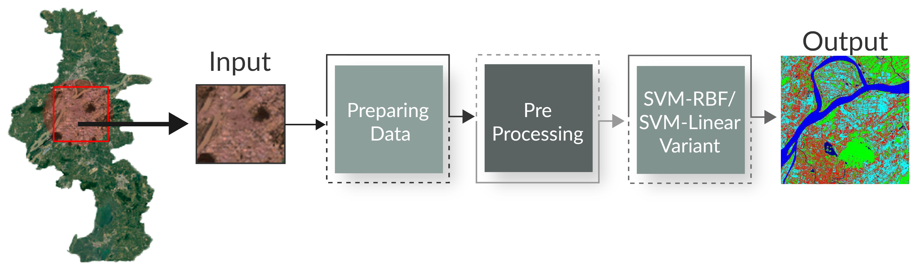
- Novel framework based on SVM-RBF and SVM-Linear for the classification of remote sensing images have been introduced to improve the accuracy and efficiency and overcome many existing challenges.
- The proposed SVM-RBF and SVM-Linear are capable to address mask generation, cross-validation, ranking, change classification/No-change classification, underfitting, and overfitting.
- SVM-Linear and non-linear SVM-RBF can minimize the computational load by separating the samples from different classes.
- The SVM-RBF and SVM-Linear are also compared with the state-of-the-art algorithms (NDCI, SCMask R-CNN, CIAs, KCA, and AOPC from the change detection accuracy, and reliability perspective. The proposed SVM-RBF and SVM-Linear have shown higher overall accuracy and better reliability compared to existing approaches.
2. Literature Review
3. Materials and Methods
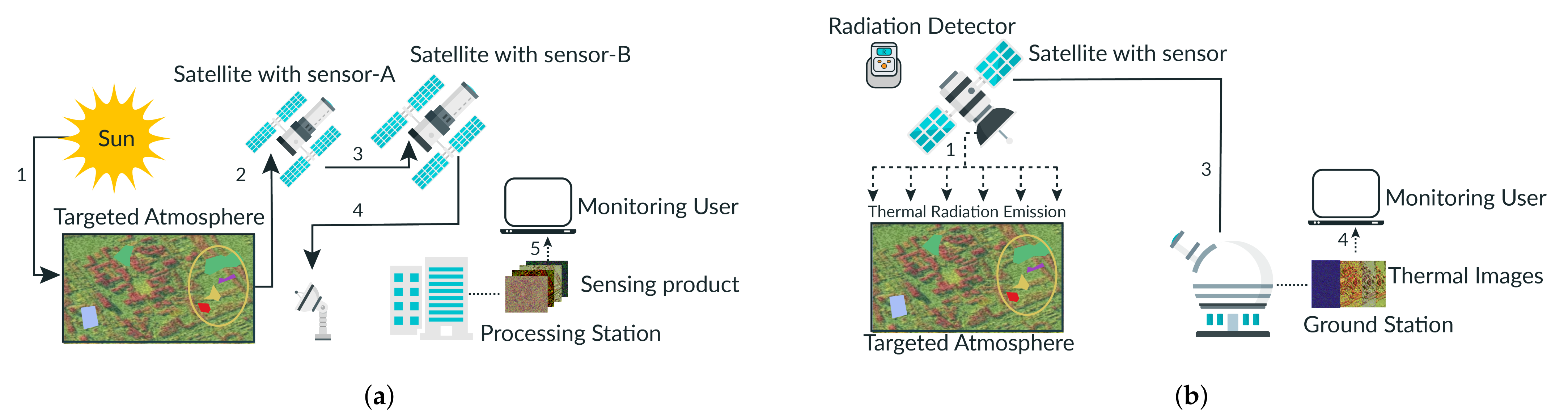
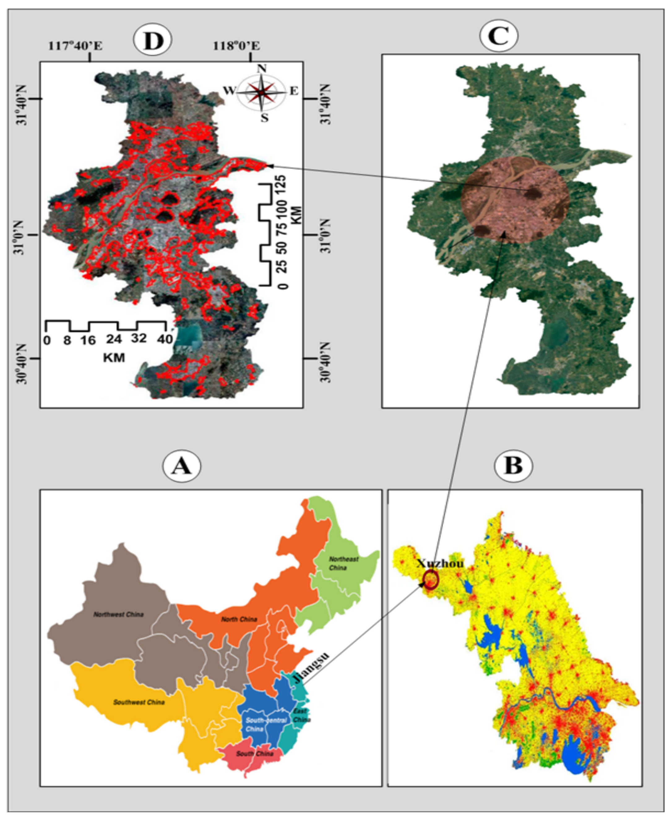
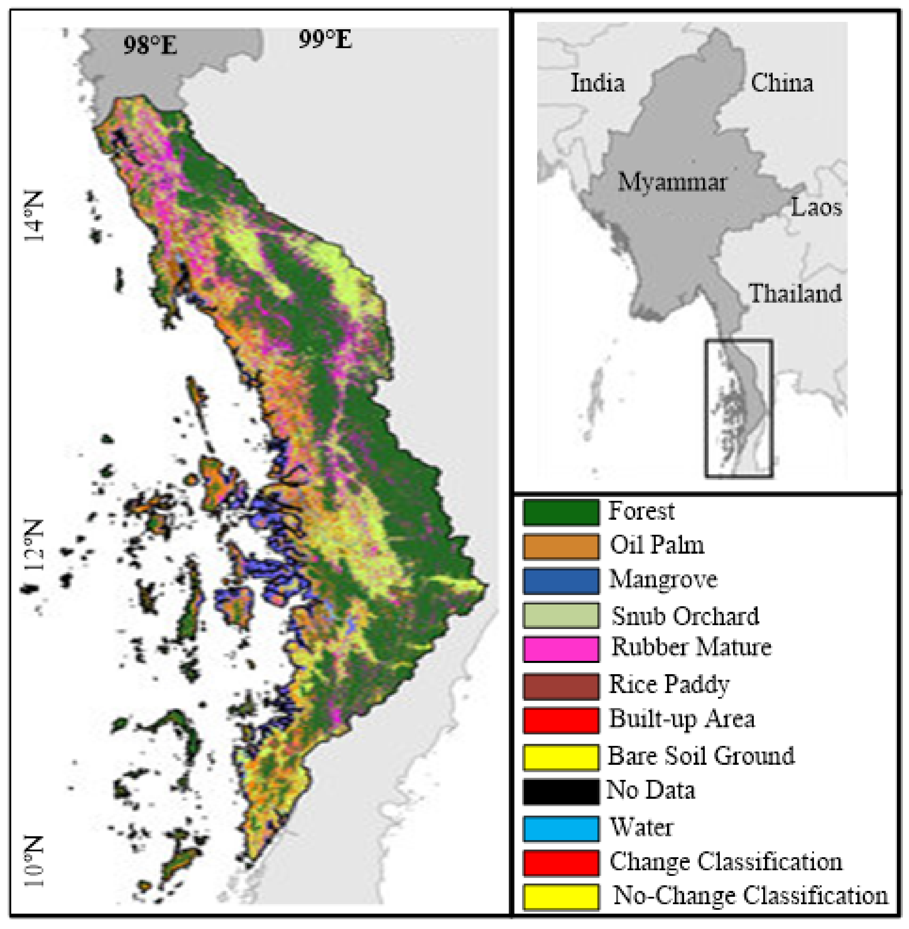
3.1. Datasets
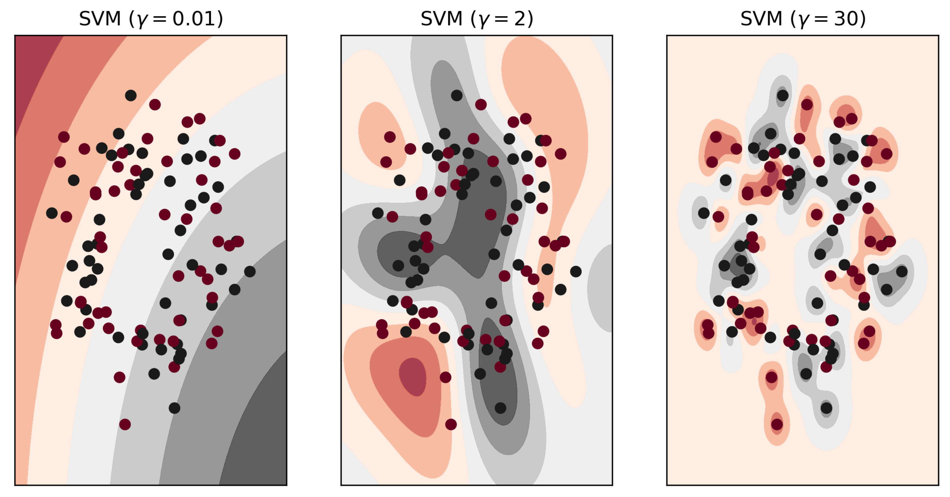
3.2. Parameters in SVM-RBF and SVM-Linear Variants
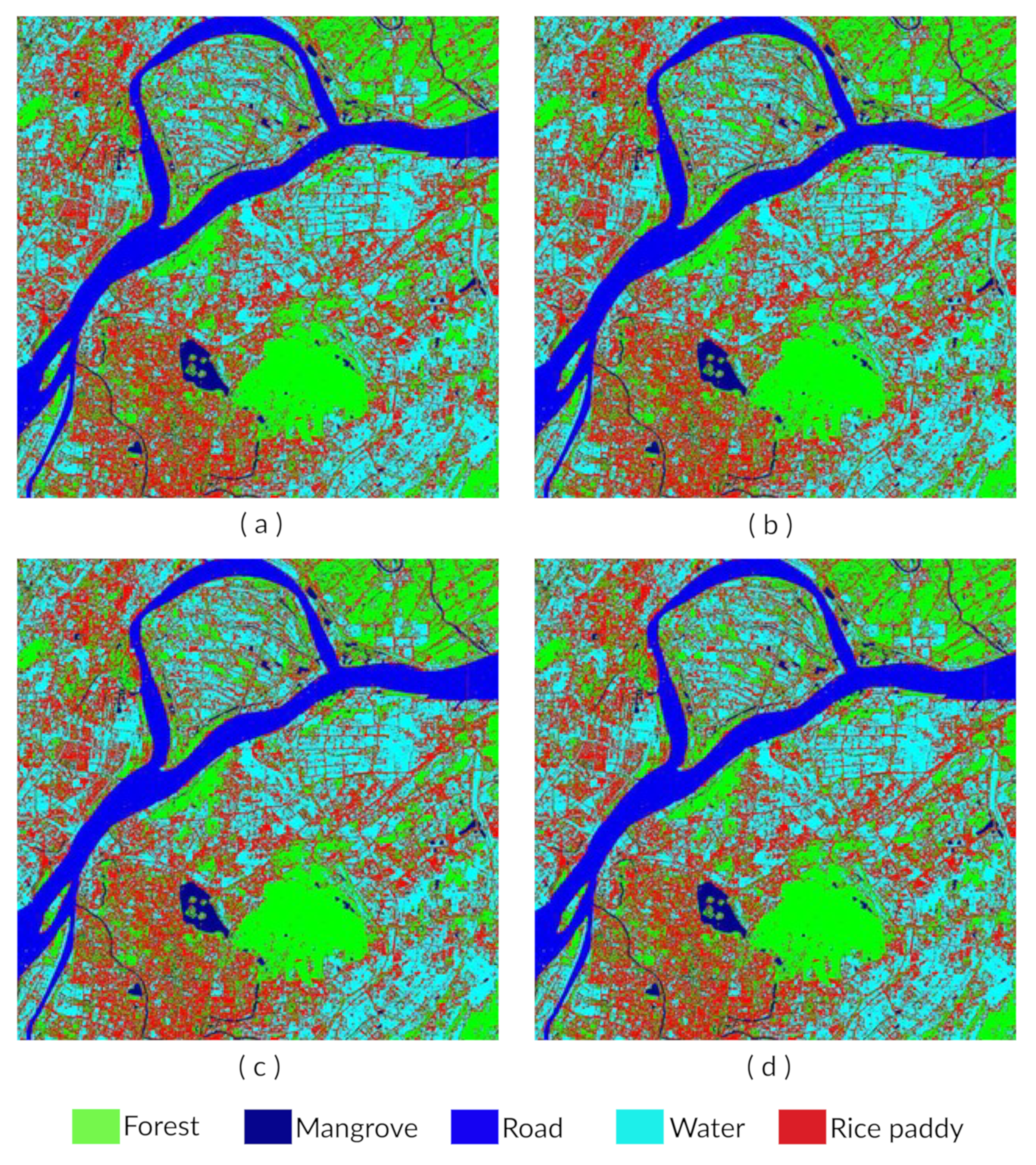
3.3. Image Processing
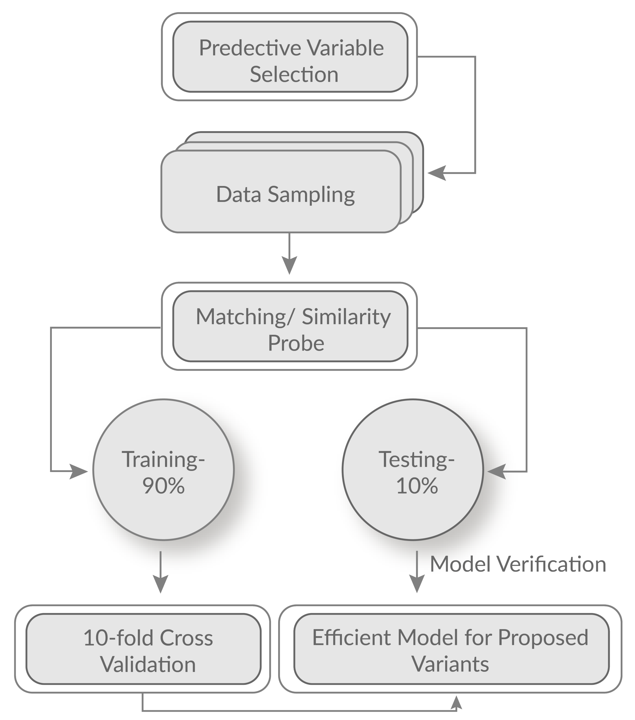
3.4. Selection of Training Test and Testing Set
3.5. Separability
3.6. Supervised Calculation
4. Mathematical Modeling and Characterization of MDC and MLC
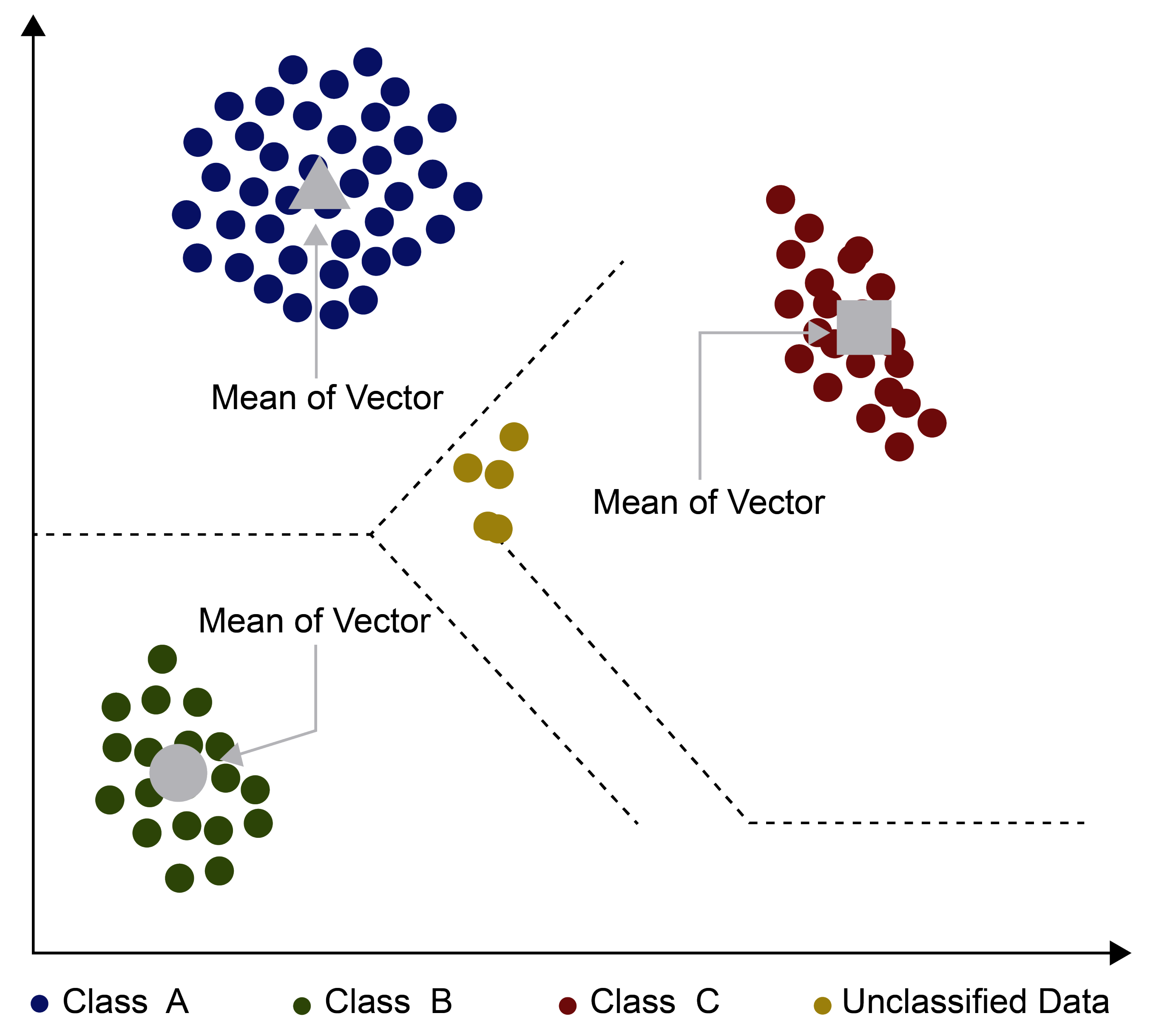
4.1. Minimum Distance Classification
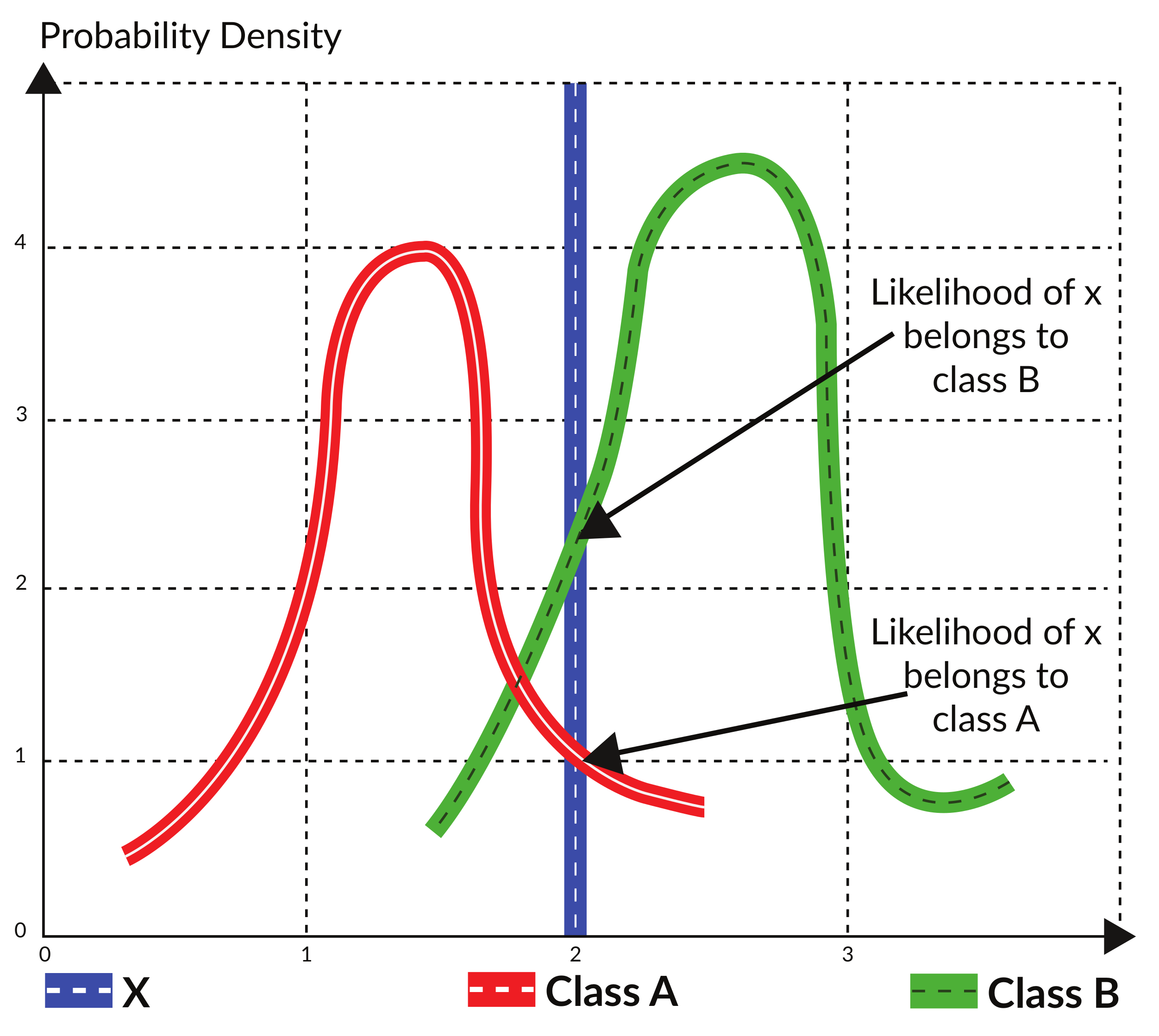
4.2. Maximum Likelihood Classification
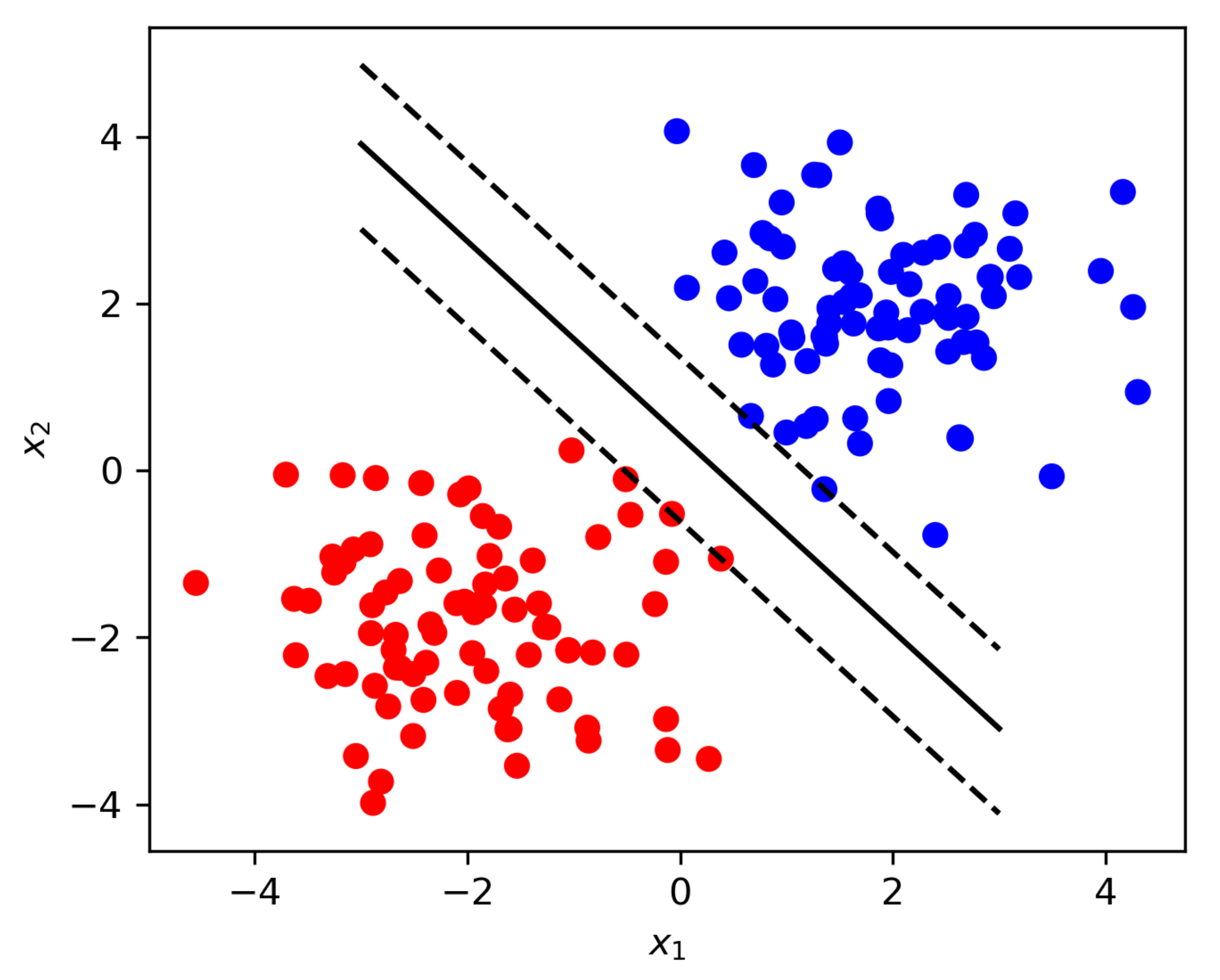
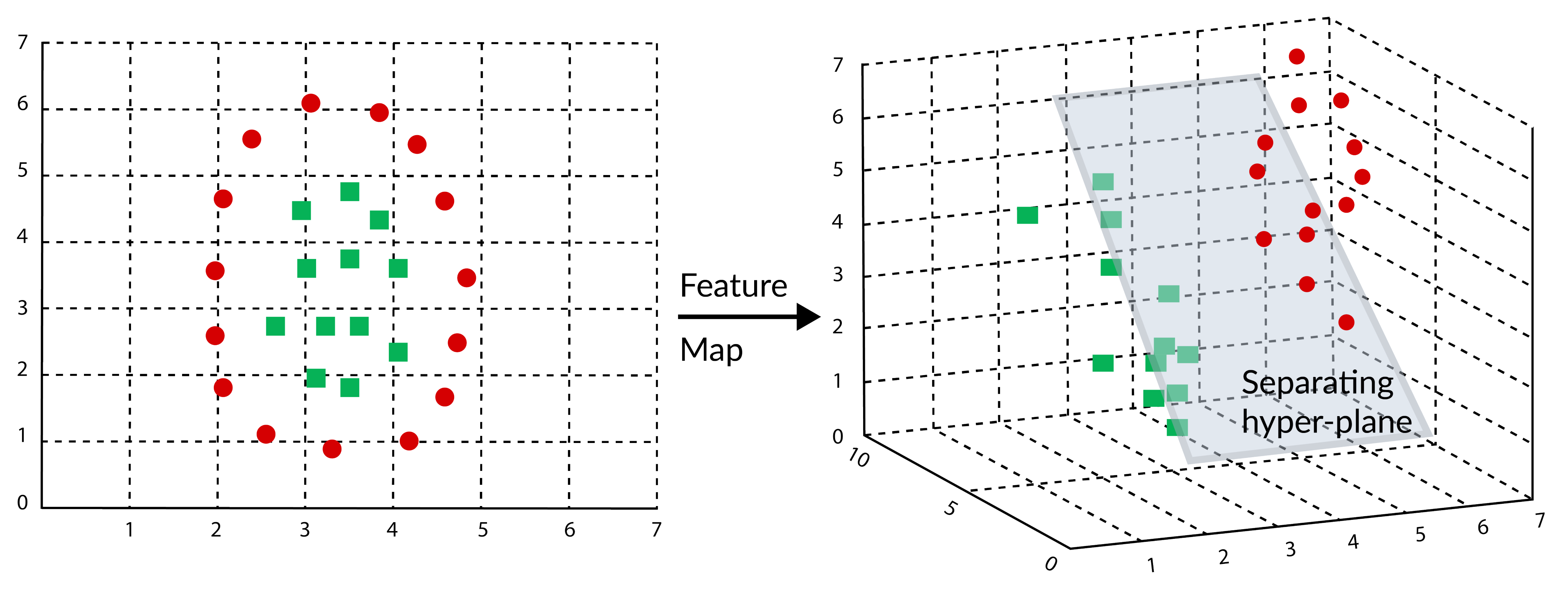
4.3. Novel Working Principles of SVM-RBF and SVM-Linear

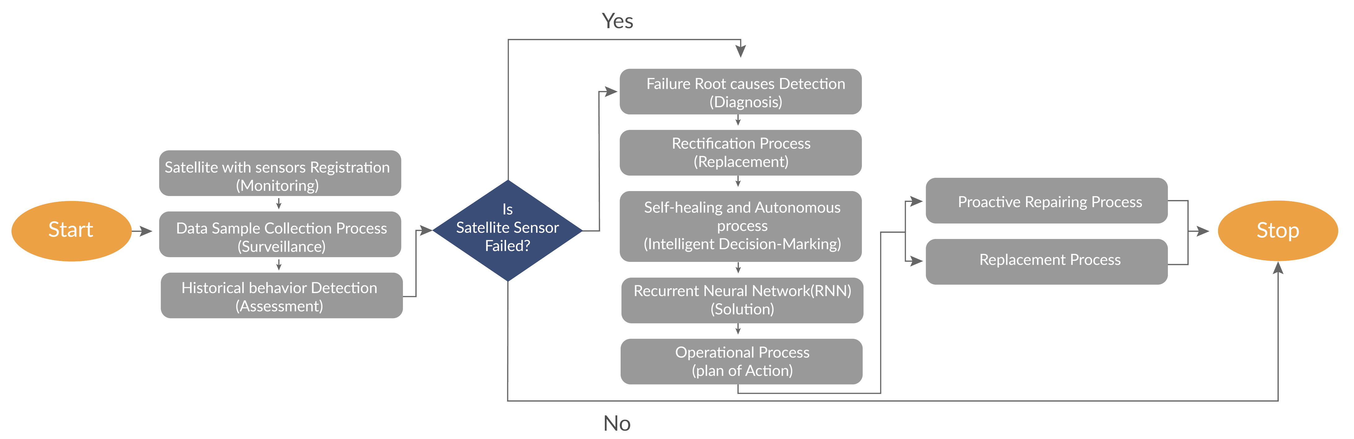
4.4. Fault-Tolerance Process of SVM-RBF and SVM-Linear
5. Experimental Results
5.1. Experimental Setup
5.2. Performance Metrics
- Accuracy;
- Time complexity;
- Fault tolerance;
- Reliability.
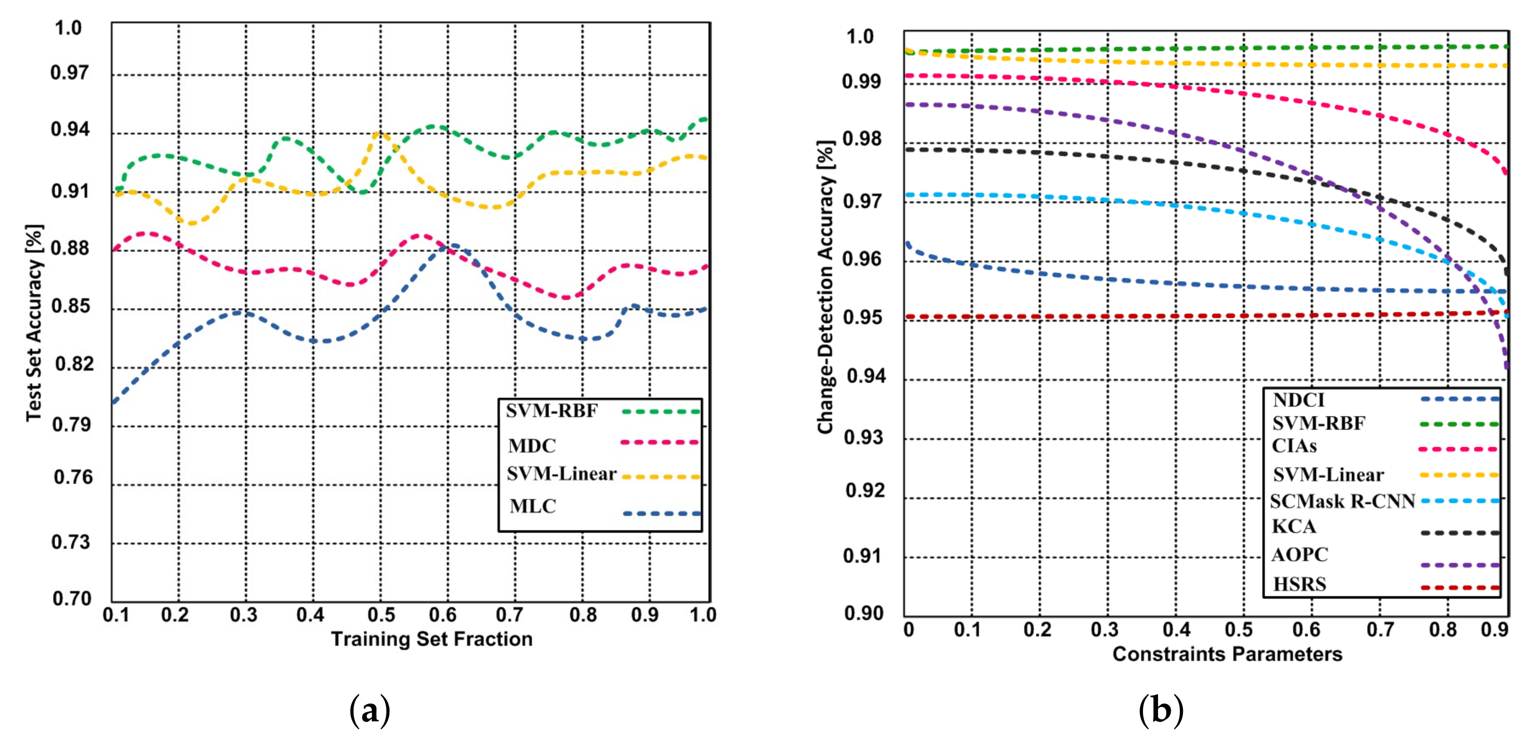
5.2.1. Accuracy
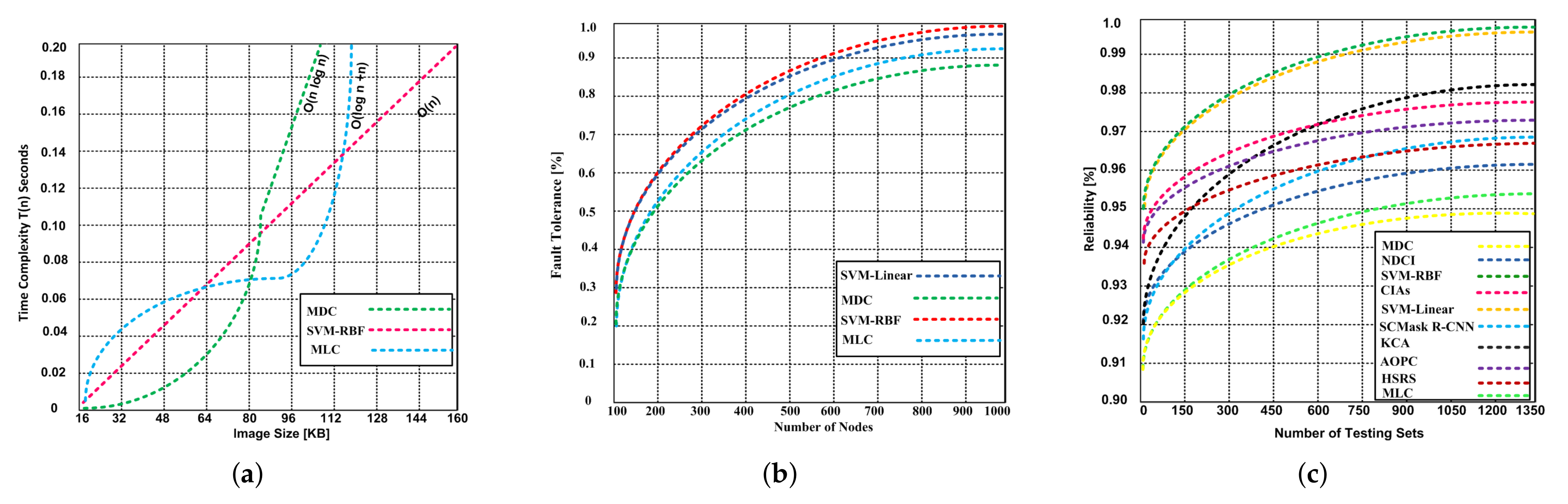
5.2.2. Time Complexity
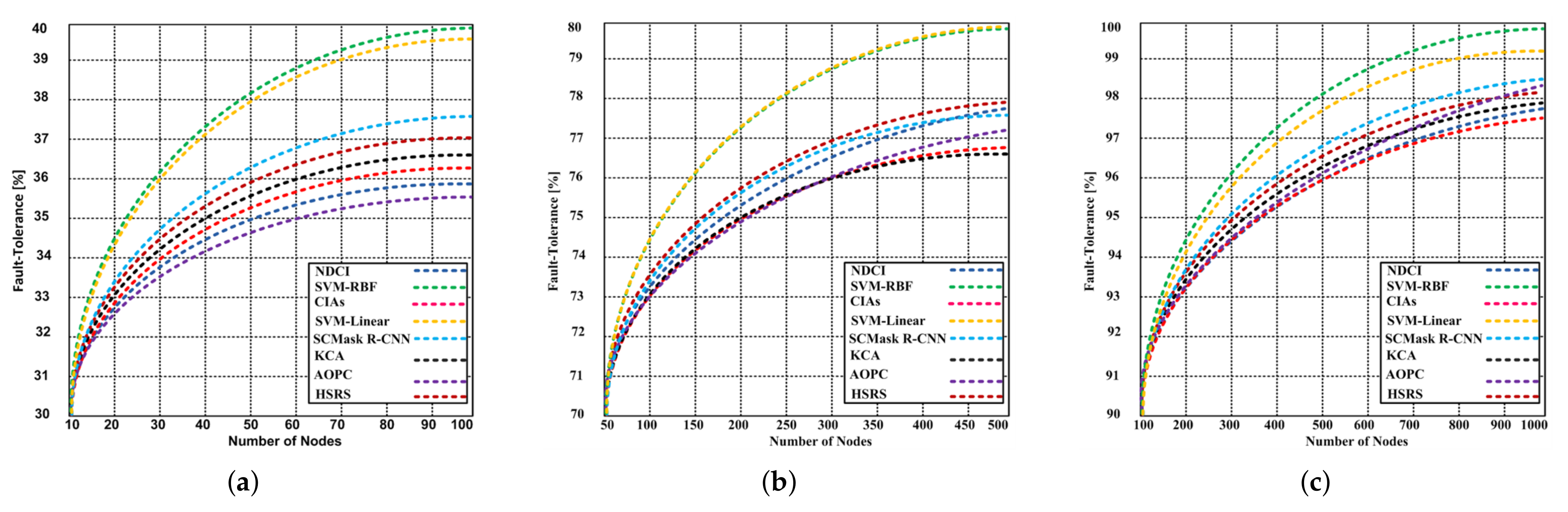
5.2.3. Fault Tolerance
5.2.4. Reliability
6. Conclusions and Future Analysis
6.1. Conclusions
- The proposed variants are capable to address mask generation, cross-validation, ranking. change classification/No-change classification, underfitting, and overfitting.
- The SVM-RBF and SVM-Linear are compared with the state-of-the-art algorithms (NDCI, SCMask R-CNN, CIAs, KCA, HSRS, and AOPC from the change detection accuracy, and reliability standpoint. The proposed SVM-RBF and SVM-Linear have obtained 99.65% and 99.43% change-detection accuracy respectively; whereas the NDCI, CIAs, SCMask R-CNN, KCA, HSRS, and AOPC have obtained the change-detection accuracy 95.6%, 97.4%, 95.0%, 95.8%, 95.2%, and 94.2% respectively.
- The SVM-RBF and SVM-Linear variants performed well on the training data with an overall accuracy of around 94% and Kappa coefficient around 0.92 which is much higher than the MDC and MLC algorithms.
- The SVM-RBF has 99.99% fault tolerance capability with 1000 nodes, whereas the MDC and MLC have 88.12% and 92.32% respectively.
- The SVM-RBF and SVM-Linear show 99.92% reliability, while the contending algorithms exhibit 93.8–98.2% reliability. The MDC and MLC produce the lower 93.8% and 95.4% reliability respectively.
- The SVM-RBF produces O(n) time complexity that is reasonable with remote image sensing.
- SVM-RBF obtains good generalization performance on unknown data and is more suitable for practical use than traditional parametric classifiers.
- The time spent by the SVM-RBF is much lower than the MLC and MDC, especially in the cross-validation for parameter optimization.
6.2. Future Work
Author Contributions
Funding
Institutional Review Board Statement
Informed Consent Statement
Data Availability Statement
Conflicts of Interest
Abbreviations
| RS | Remote sensing |
| SVM | Support vector machine |
| MCD | Minimum distance classification |
| MLC | Maximum likelihood classification |
| ASTER | Advanced spaceborne thermal emission and reflection |
| TM | Thematic mapper |
| DT | Decision tree |
| RBF | Radial basis function |
| ROI | Region of interest |
| IDL | Interactive data language |
| ENVI | Environment for visualizing images |
| OVA | One versus all |
| CNN | Convolutional neural network |
| NA | Not applicable |
| M | Number of classes |
| Kernel parameter to determine how many nearby samples the support vector will | |
| consider | |
| C | Penalty factor used for regularization |
| Number of training data | |
| Class | |
| x | Pixel |
| Euclidean distance | |
| A posteriori distribution | |
| Prior probability | |
| The probability that class occurs in the study area | |
| The probability that pixel x is observed | |
| The probability density function of normal distribution in an n-dimensional space | |
| The covariance matrix of the M bands in kth class | |
| Overall accuracy | |
| Partial accuracy | |
| Probability estimated when sensor/actor are not faulty | |
| Binary variable with decoder value | |
| Sensor-reading | |
| Ground truth | |
| K of the sensor/actor nodes that have same reading | |
| Conditional probability | |
| Not faulty neighbors | |
| Average number of errors after decoding | |
| Number of other nodes | |
| Nodes in the affected region | |
| Expected faulty nodes | |
| Total deployed nodes in the network | |
| Average number of corrected faults | |
| Number of uncorrected faults | |
| Reliability | |
| Functioning probability of either actor/sensor node | |
| Reliability of total components used in the network |
Appendix A

| Methods | Time Complexity |
|---|---|
| SVM-RBF | |
| Problem consists of finite set of inputs, but its computation time linearly increases. Thus, | |
| Where t is ignored; therefore | |
| MDC | |
| Where problem is divided into two parts with same size. However, the algorithm is infinite. Thus. | |
| Where | |
| MLC | |
| Problem consists of finite set of inputs, but computation complexity remains constant n | |
| : | |
| : | |
| Where t is ignored; therefore, we get | |
References
- Barmpoutis, P.; Papaioannou, P.; Dimitropoulos, K.; Grammalidis, N. A Review on Early Forest Fire Detection Systems Using Optical Remote Sensing. Sensors 2020, 20, 6442. [Google Scholar] [CrossRef]
- Van Natijne, A.L.; Lindenbergh, R.C.; Bogaard, T.A. Machine learning: New potential for local and regional deep-seated landslide nowcasting. Sensors 2020, 20, 1425. [Google Scholar] [CrossRef] [Green Version]
- Yang, C. Remote sensing and precision agriculture technologies for crop disease detection and management with a practical application example. Engineering 2020, 6, 528–532. [Google Scholar] [CrossRef]
- Li, W.; Xiang, M.; Liang, X. MDCwFB: A Multilevel Dense Connection Network with Feedback Connections for Pansharpening. Remote Sens. 2021, 13, 2218. [Google Scholar] [CrossRef]
- Talukdar, S.; Singha, P.; Mahato, S.; Shahfahad; Pal, S.; Liou, Y.-A.; Rahman, A. Land-Use Land-Cover Classification by Machine Learning Classifiers for Satellite Observations—A Review. Remote Sens. 2020, 12, 1135. [Google Scholar] [CrossRef] [Green Version]
- Shaharum, N.S.N.; Shafri, H.Z.M.; Gambo, J.; Abidin, F.A.Z. Mapping of Krau Wildlife Reserve (KWR) protected area using Landsat 8 and supervised classification algorithms. Remote Sens. Appl. Soc. Environ. 2018, 10, 24–35. [Google Scholar] [CrossRef]
- Zhao, Q.; Jia, S.; Li, Y. Hyperspectral remote sensing image classification based on tighter random projection with minimal intra-class variance algorithm. Pattern Recognit. 2021, 111, 107635. [Google Scholar] [CrossRef]
- Rahiche, A.; Hedjam, R.; Al-maadeed, S.; Cheriet, M. Historical documents dating using multispectral imaging and ordinal classification. J. Cult. Herit. 2020, 45, 71–80. [Google Scholar] [CrossRef]
- Liu, C.A.; Chen, Z.X.; Yun, S.H.A.O.; Chen, J.S.; Hasi, T.; Pan, H.Z. Research advances of SAR remote sensing for agriculture applications: A review. J. Integr. Agric. 2019, 18, 506–525. [Google Scholar] [CrossRef] [Green Version]
- Liu, Y.; Hu, C.; Dong, Y.; Xu, B.; Zhan, W.; Sun, C. Geometric accuracy of remote sensing images over oceans: The use of global offshore platforms. Remote Sens. Environ. 2019, 222, 244–266. [Google Scholar] [CrossRef]
- Pati, C.; Panda, A.K.; Tripathy, A.K.; Pradhan, S.K.; Patnaik, S. A novel hybrid machine learning approach for change detection in remote sensing images. Eng. Sci. Technol. Int. J. 2020, 23, 973–981. [Google Scholar] [CrossRef]
- Oh, Y.; Ransikarbum, K.; Busogi, M.; Kwon, D.; Kim, N. Adaptive SVM-based real-time quality assessment for primer-sealer dispensing process of sunroof assembly line. Reliab. Eng. Syst. Saf. 2019, 184, 202–212. [Google Scholar] [CrossRef]
- Tan, Q.; Guo, B.; Hu, J.; Dong, X.; Hu, J. Object-oriented remote sensing image information extraction method based on multi-classifier combination and deep learning algorithm. Pattern Recognit. Lett. 2021, 141, 32–36. [Google Scholar] [CrossRef]
- Quemy, A. Binary classification in unstructured space with hypergraph case-based reasoning. Inf. Syst. 2019, 85, 92–113. [Google Scholar] [CrossRef] [Green Version]
- Jin, X.; Jin, Y.; Mao, X. Ecological risk assessment of cities on the Tibetan Plateau based on land use/land cover changes—Case study of Delingha City. Ecol. Indic. 2019, 101, 185–191. [Google Scholar] [CrossRef]
- Glowacz, A. Ventilation Diagnosis of Angle Grinder Using Thermal Imaging. Sensors 2021, 21, 2853. [Google Scholar] [CrossRef]
- Wu, Q.; Feng, D.; Cao, C.; Zeng, X.; Feng, Z.; Wu, J.; Huang, Z. Improved Mask R-CNN for Aircraft Detection in Remote Sensing Images. Sensors 2021, 21, 2618. [Google Scholar] [CrossRef]
- Zhong, Y.; Ma, A.; Soon Ong, Y.; Zhu, Z.; Zhang, L. Computational intelligence in optical remote sensing image processing. Appl. Soft Comput. 2018, 64, 75–93. [Google Scholar] [CrossRef]
- Huang, F.; Yu, Y.; Feng, T. Hyperspectral remote sensing image change detection based on tensor and deep learning. J. Vis. Commun. Image Represent. 2019, 58, 233–244. [Google Scholar] [CrossRef]
- Xu, J.; Feng, G.; Zhao, T.; Sun, X.; Zhu, M. Remote sensing image classification based on semi-supervised adaptive interval type-2 fuzzy c-means algorithm. Comput. Geosci. 2019, 131, 132–143. [Google Scholar] [CrossRef]
- Ge, G.; Shi, Z.; Zhu, Y.; Yang, X.; Hao, Y. Land use/cover classification in an arid desert-oasis mosaic landscape of China using remote sensed imagery: Performance assessment of four machine learning algorithms. Glob. Ecol. Conserv. 2020, 22, e00971. [Google Scholar] [CrossRef]
- Arief, H.A.A.; Indahl, U.G.; Strand, G.H.; Tveite, H. Addressing overfitting on point cloud classification using Atrous XCRF. ISPRS J. Photogramm. Remote Sens. 2019, 155, 90–101. [Google Scholar] [CrossRef] [Green Version]
- Myint Oo, M.; Kamolphiwong, S.; Kamolphiwong, T.; Vasupongayya, S. Advanced support vector machine-(ASVM-) based detection for distributed denial of service (DDoS) attack on software defined networking (SDN). J. Comput. Networks Commun. 2019, 2019, 8012568. [Google Scholar] [CrossRef] [Green Version]
- Chen, Y.; Wei, Y.; Wang, Q.; Chen, F.; Lu, C.; Lei, S. Mapping Post-Earthquake Landslide Susceptibility: A U-Net Like Approach. Remote Sens. 2020, 12, 2767. [Google Scholar] [CrossRef]
- Gasmi, A.; Gomez, C.; Lagacherie, P.; Zouari, H.; Laamrani, A.; Chehbouni, A. Mean spectral reflectance from bare soil pixels along a Landsat-TM time series to increase both the prediction accuracy of soil clay content and mapping coverage. Geoderma 2021, 388, 114864. [Google Scholar] [CrossRef]
- Mahmud, M.S.; Nandan, V.; Howell, S.E.; Geldsetzer, T.; Yackel, J. Seasonal evolution of L-band SAR backscatter over landfast Arctic sea ice. Remote Sens. Environ. 2020, 251, 112049. [Google Scholar] [CrossRef]
- Vögler, R.; González, C.; Segura, A.M. Spatio-temporal dynamics of the fish community associated with artisanal fisheries activities within a key marine protected area of the Southwest Atlantic (Uruguay). Ocean. Coast. Manag. 2020, 190, 105175. [Google Scholar] [CrossRef]
- Asad, M.H.; Bais, A. Weed detection in canola fields using maximum likelihood classification and deep convolutional neural network. Inf. Process. Agric. 2019, 7, 535–545. [Google Scholar] [CrossRef]
- Tian, H.; Wang, T.; Liu, Y.; Qiao, X.; Li, Y. Computer vision technology in agricultural automation—A review. Inf. Process. Agric. 2020, 7, 1–19. [Google Scholar] [CrossRef]
- Torabi, M.; Hashemi, S.; Saybani, M.R.; Shamshirband, S.; Mosavi, A. A Hybrid clustering and classification technique for forecasting short-term energy consumption. Environ. Prog. Sustain. Energy 2019, 38, 66–76. [Google Scholar] [CrossRef] [Green Version]
- Zhang, C.; Sargent, I.; Pan, X.; Li, H.; Gardiner, A.; Hare, J.; Atkinson, P.M. Joint Deep Learning for land cover and land use classification. Remote Sens. Environ. 2019, 221, 173–187. [Google Scholar] [CrossRef] [Green Version]
- Shahnazari, H. Fault diagnosis of nonlinear systems using recurrent neural networks. Chem. Eng. Res. Des. 2020, 153, 233–245. [Google Scholar] [CrossRef]
- Huynh, H.T.; Nguyen, L. Nonparametric maximum likelihood estimation using neural networks. Pattern Recognit. Lett. 2020, 138, 580–586. [Google Scholar] [CrossRef]
- Shokrzade, A.; Ramezani, M.; Tab, F.A.; Mohammad, M.A. A novel extreme learning machine based kNN classification method for dealing with big data. Expert Syst. Appl. 2021, 2021, 115293. [Google Scholar] [CrossRef]
- Zhang, L.; Wu, J.; Fan, Y.; Gao, H.; Shao, Y. An efficient building extraction method from high spatial resolution remote sensing images based on improved mask R-CNN. Sensors 2020, 20, 1465. [Google Scholar] [CrossRef] [PubMed] [Green Version]
- Zhang, J.; Zhang, W.; Mei, Y.; Yang, W. Geostatistical characterization of local accuracies in remotely sensed land cover change categorization with complexly configured reference samples. Remote. Sens. Environ. 2019, 223, 63–81. [Google Scholar] [CrossRef]
- Varatharajan, R.; Vasanth, K.; Gunasekaran, M.; Priyan, M.; Gao, X.Z. An adaptive decision based kriging interpolation algorithm for the removal of high density salt and pepper noise in images. Comput. Electr. Eng. 2018, 70, 447–461. [Google Scholar] [CrossRef]


| Characteristics/Features | NDCI [8] | R-CNN [17] | CIAs [18] | HSRS [19] | KCA [21] | AOPC [22] | Proposed Method |
|---|---|---|---|---|---|---|---|
| Segmentation/Preprocessing | No | Yes | Yes | No | Yes | No | Yes |
| Separability | No | No | Yes | No | No | Yes | Yes |
| Ranking Classification | Yes | Yes | No | Yes | No | No | Yes |
| Change Classification | Yes | No | Yes | Yes | Yes | Yes | Yes |
| No-Change Classification | No | No | No | Yes | No | No | Yes |
| Image Classification | Yes | No | Yes | Yes | Yes | Yes | Yes |
| Visual interpretation and Field Verification | No | Yes | No | Yes | No | No | Yes |
| Feature Mapping | No | Yes | No | Yes | Yes | No | Yes |
| Dealing with unlabeled samples | No | No | No | Yes | No | Yes | No |
| Deal with underfitting and Overfitting | No | No | No | No | Yes | Yes | Yes |
| Addressing Generalization Problem | No | No | Yes | No | No | No | Yes |
| Forest Detection | No | No | Yes | Yes | Yes | Yes | Yes |
| Bare Soil Ground Detection | Yes | No | No | Yes | Yes | No | Yes |
| Water Detection | No | No | Yes | No | Yes | No | Yes |
| Urbanization Region Detection | Yes | Yes | No | Yes | Yes | Yes | Yes |
| Cross validation Process | No | Yes | No | No | No | Yes | Yes |
| Mask Generation Process | No | Yes | No | Yes | No | - | Yes |
| Change Detection Accuracy | 95.6% | 95.1% | 97.4% | 95.2% | 95.8% | 94.2% | SVM-RBF = 99.65%, |
| SVM-Linear = 99.43% |
| Classifier/Criteria | Test Accuracy | Test Kappa Coefficient |
|---|---|---|
| MDC | 72.82 | 0.64 |
| MLC | 80.03 | 0.74 |
| SVM-Linear | 81.33 | 0.75 |
| Default SVM-RBF (C = 100, r = 0.33) | 85.40 | 0.80 |
| Improved SVM-RBF | 89.32 | 0.84 |
| Parameters | Values |
|---|---|
| MDC | 72.82 |
| Sensing time | 2.5 milliseconds |
| Sensing samples | 250 |
| Kernel functions | Linear and RBF kernels |
| Training observation | 1000 |
| Testing observation | 6000 |
| Source of sensing Images | Landsat 8 |
| Cross-validation | 5 |
Publisher’s Note: MDPI stays neutral with regard to jurisdictional claims in published maps and institutional affiliations. |
© 2021 by the authors. Licensee MDPI, Basel, Switzerland. This article is an open access article distributed under the terms and conditions of the Creative Commons Attribution (CC BY) license (https://creativecommons.org/licenses/by/4.0/).
Share and Cite
Razaque, A.; Ben Haj Frej, M.; Almi’ani, M.; Alotaibi, M.; Alotaibi, B. Improved Support Vector Machine Enabled Radial Basis Function and Linear Variants for Remote Sensing Image Classification. Sensors 2021, 21, 4431. https://doi.org/10.3390/s21134431
Razaque A, Ben Haj Frej M, Almi’ani M, Alotaibi M, Alotaibi B. Improved Support Vector Machine Enabled Radial Basis Function and Linear Variants for Remote Sensing Image Classification. Sensors. 2021; 21(13):4431. https://doi.org/10.3390/s21134431
Chicago/Turabian StyleRazaque, Abdul, Mohamed Ben Haj Frej, Muder Almi’ani, Munif Alotaibi, and Bandar Alotaibi. 2021. "Improved Support Vector Machine Enabled Radial Basis Function and Linear Variants for Remote Sensing Image Classification" Sensors 21, no. 13: 4431. https://doi.org/10.3390/s21134431
APA StyleRazaque, A., Ben Haj Frej, M., Almi’ani, M., Alotaibi, M., & Alotaibi, B. (2021). Improved Support Vector Machine Enabled Radial Basis Function and Linear Variants for Remote Sensing Image Classification. Sensors, 21(13), 4431. https://doi.org/10.3390/s21134431