
Mitigating Cybersickness in Virtual Reality Systems through Foveated Depth-of-Field Blur


Abstract
1. Introduction
2. Related Works
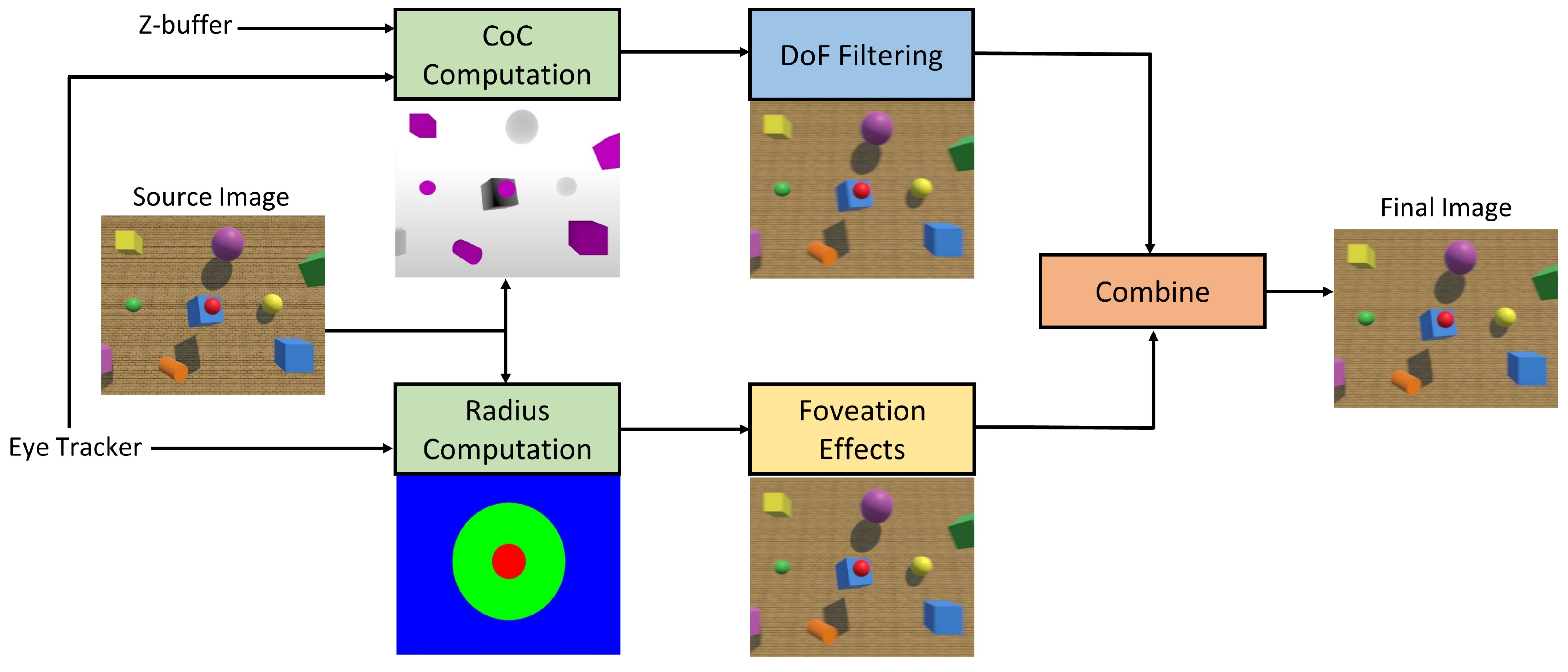
3. The Proposed Foveated Depth-of-Field Effects
| Algorithm 1: Foveated DoF effects for VR |
 |
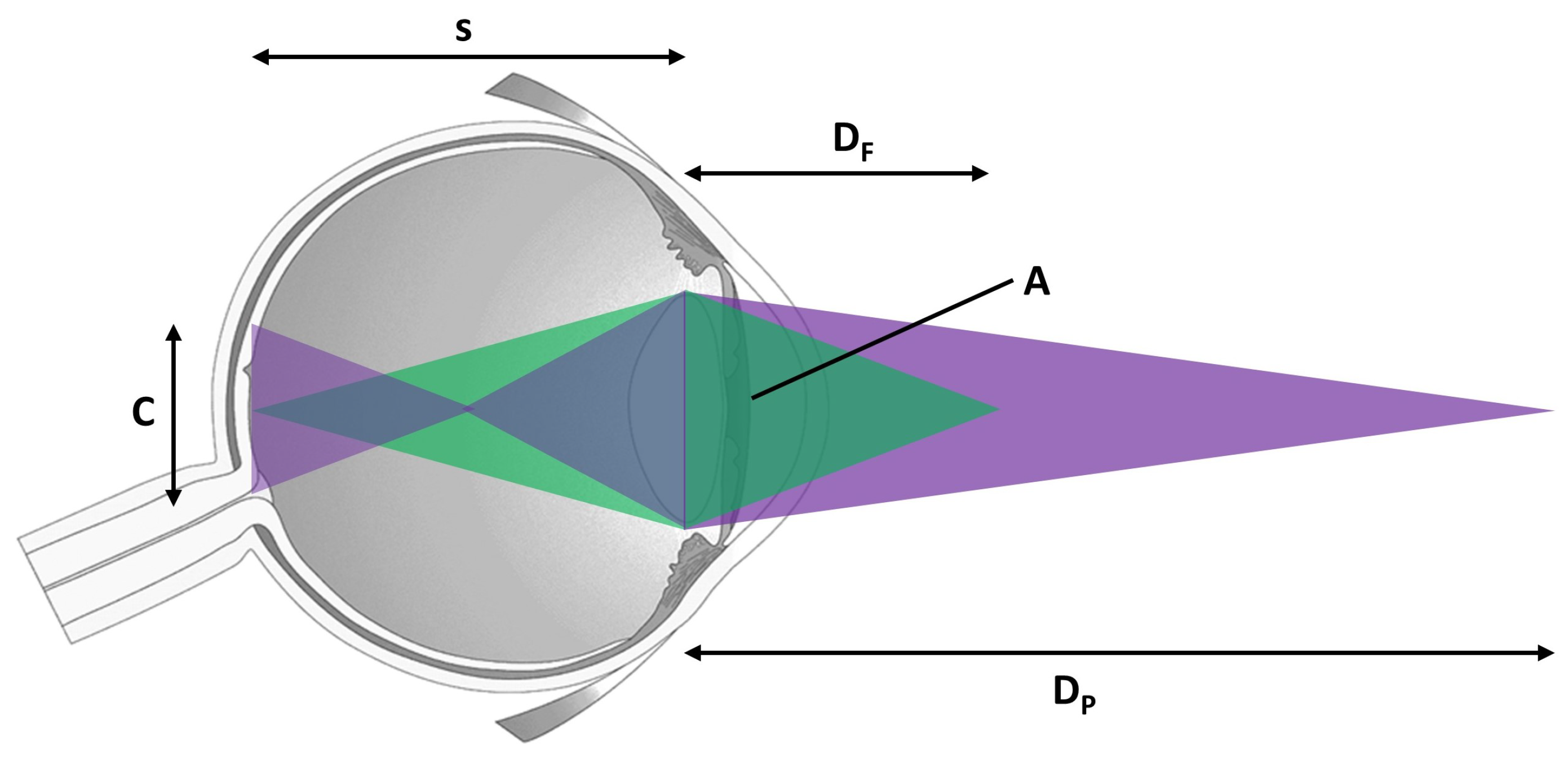
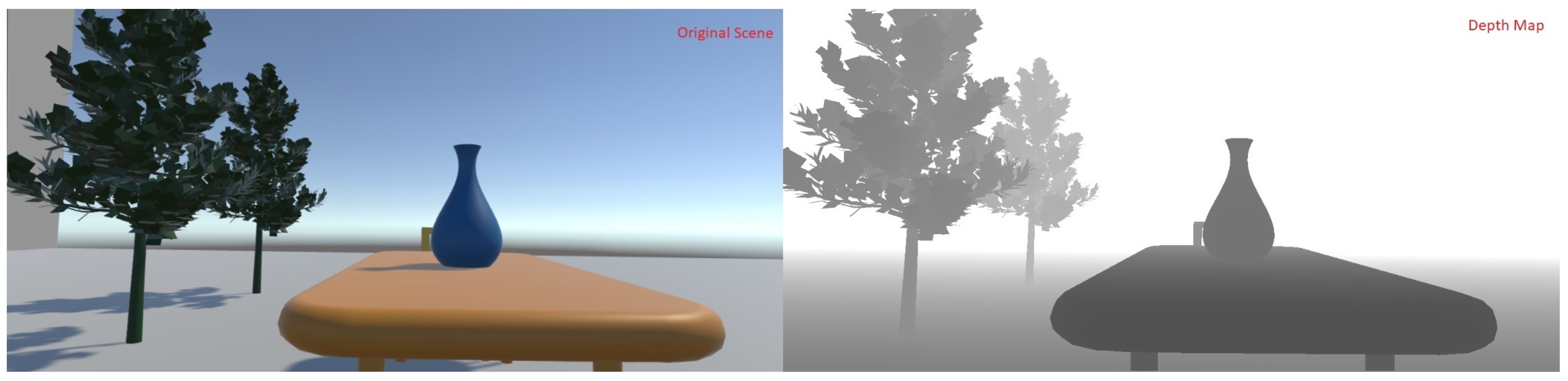
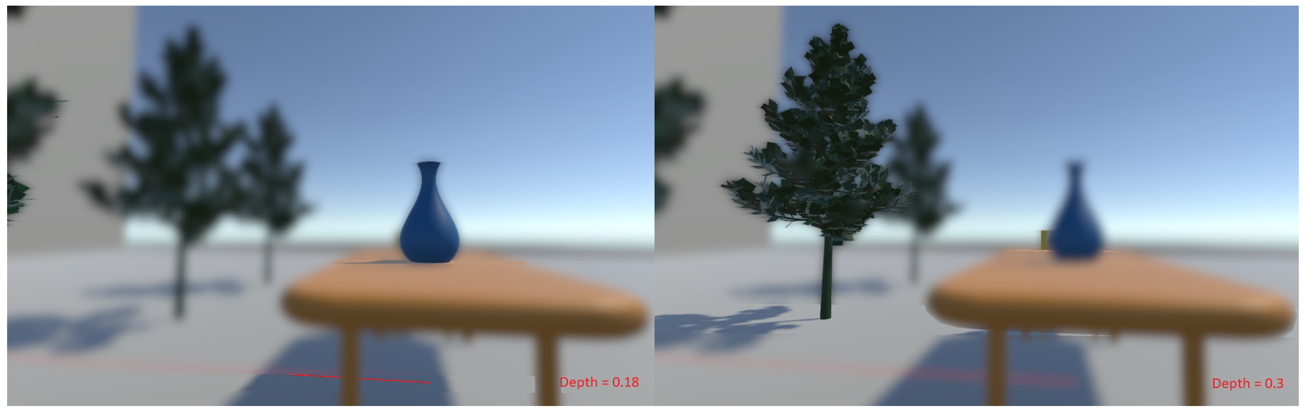
3.1. Depth-of-Field Blur
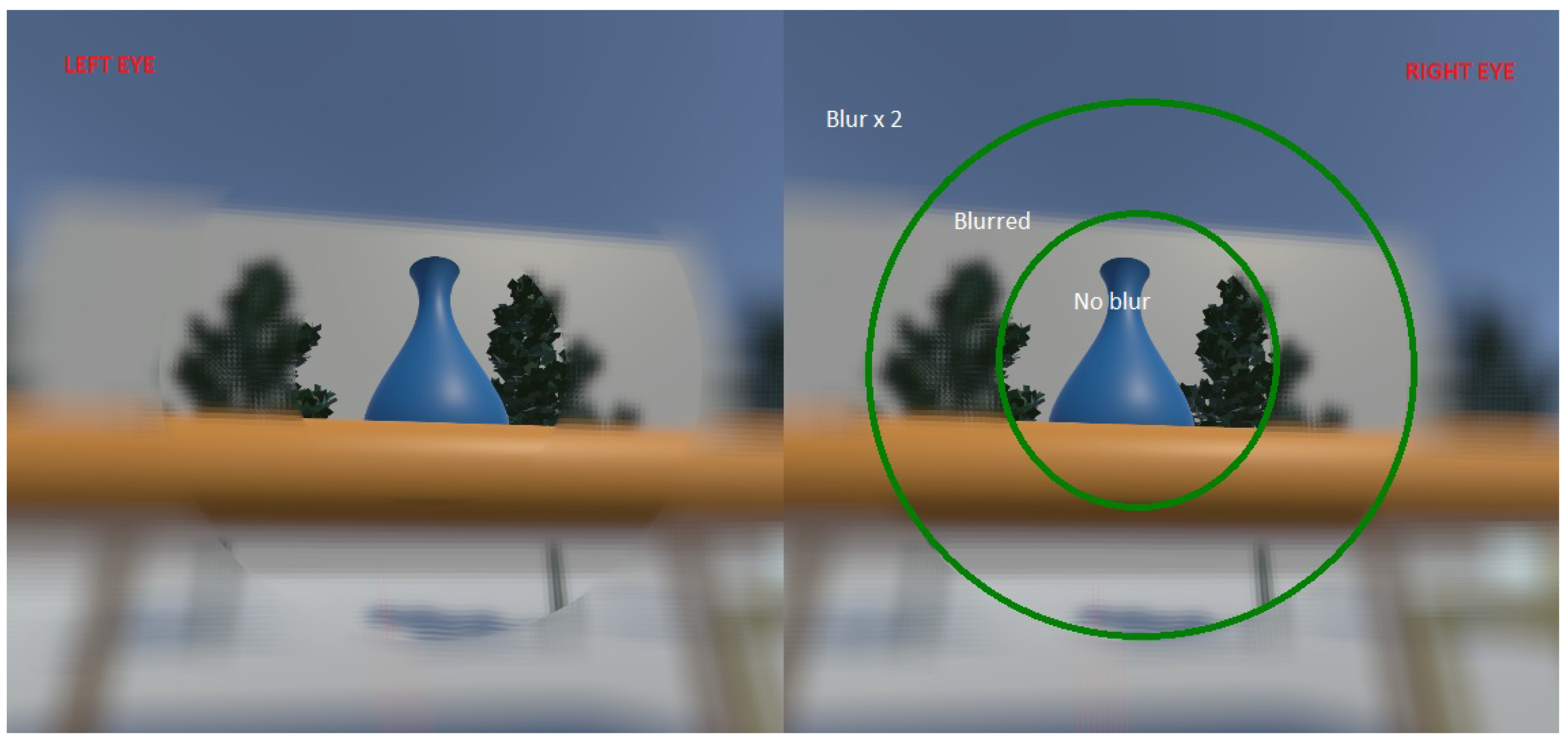
3.2. Multi-Region Foveation
3.3. Artifact Removal and Image Merging
4. User Study on Cybersickness
4.1. Participants
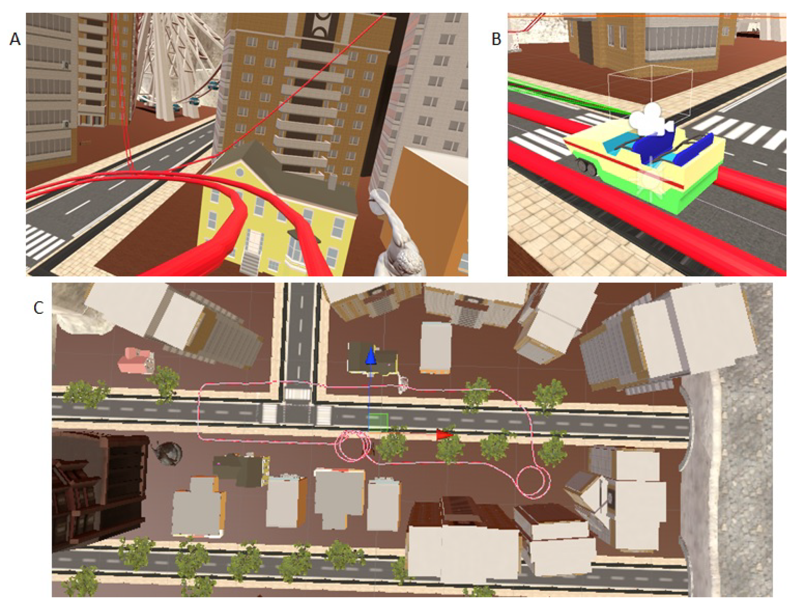
4.2. Setup
4.3. Design
4.4. Procedure
4.5. Analysis
5. Experimental Results
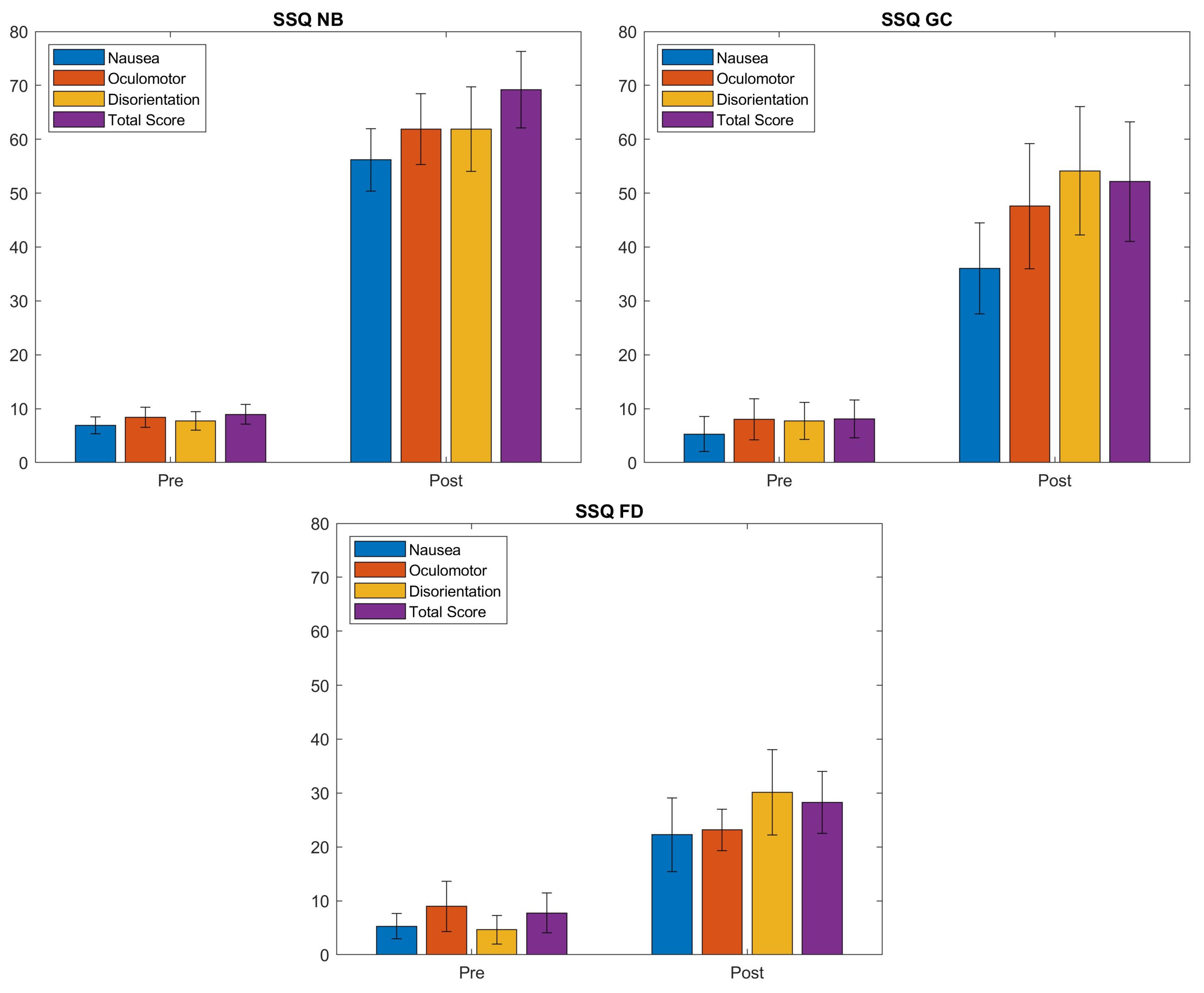
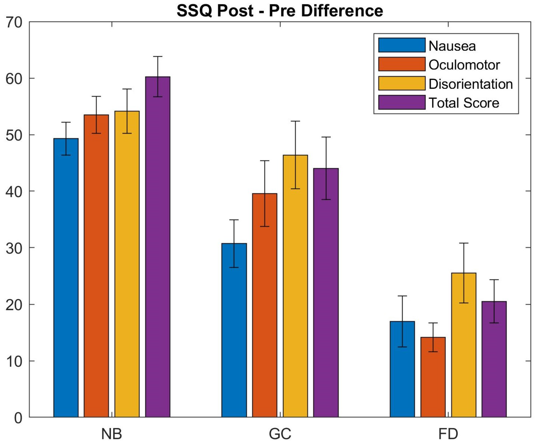
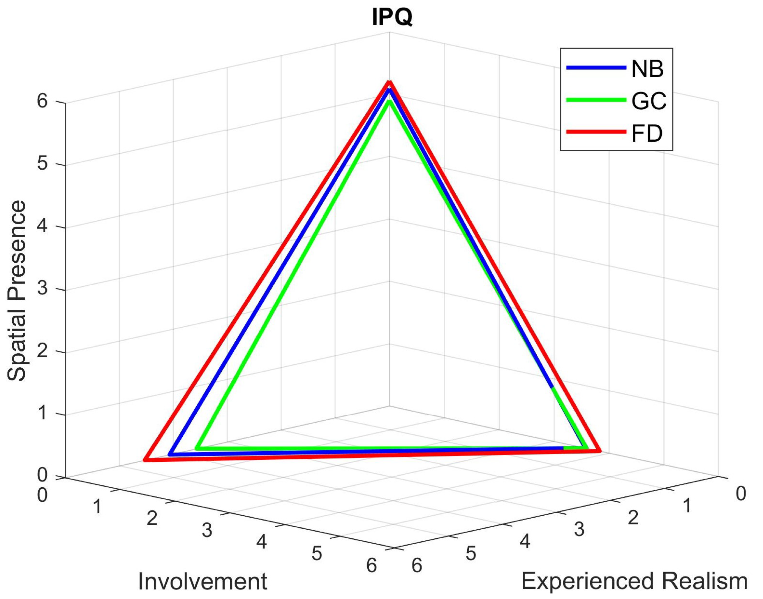
5.1. Cybersickness and Presence Evaluation
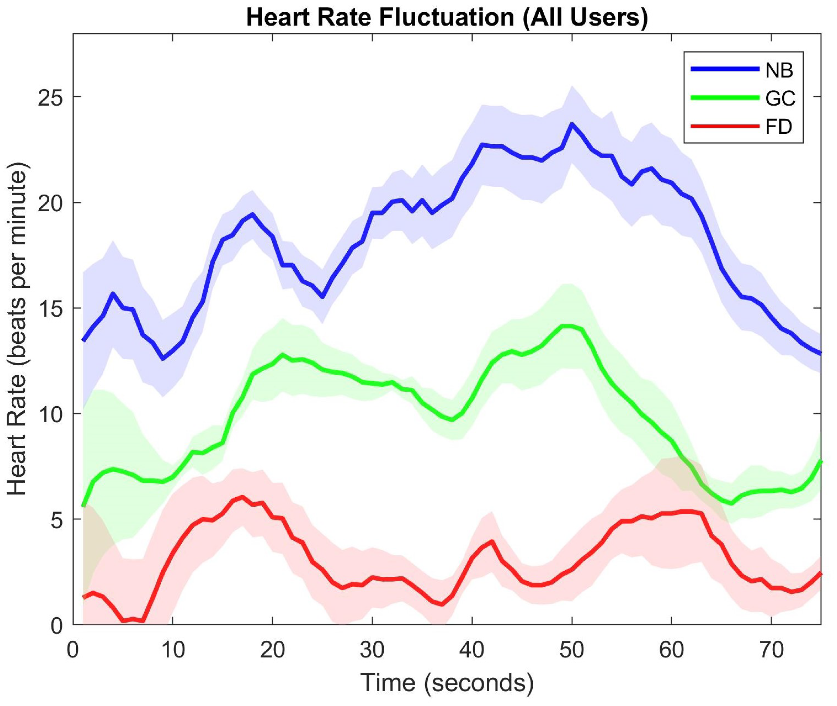
5.2. Heart Rate Observations
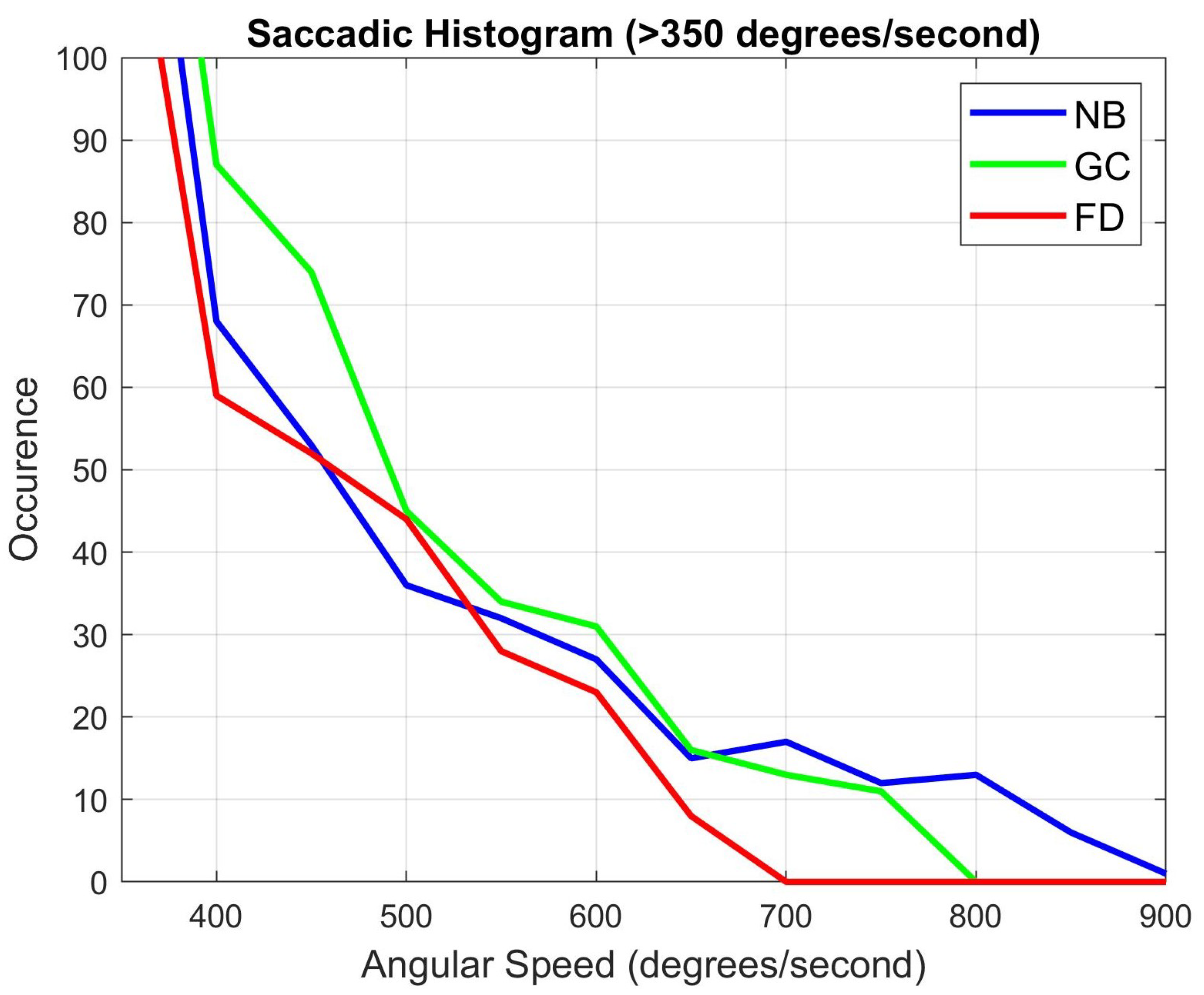
5.3. User Gaze Analysis
5.4. Age and Gender Variation
5.5. Computational Load Comparison
6. Conclusions
Author Contributions
Funding
Institutional Review Board Statement
Informed Consent Statement
Data Availability Statement
Acknowledgments
Conflicts of Interest
References
- Davis, S.; Nesbitt, K.; Nalivaiko, E. A Systematic Review of Cybersickness. In Proceedings of the 2014 Conference on Interactive Entertainment, Newcastle, NSW, Australia, 2–3 December 2014; pp. 1–9. [Google Scholar]
- Geisler, W.S. Visual Perception and the Statistical Properties of Natural Scenes. Annu. Rev. Psychol. 2008, 59, 167–192. [Google Scholar] [CrossRef] [PubMed]
- Cohen, M.A.; Dennett, D.C.; Kanwisher, N. What is the Bandwidth of Perceptual Experience? Trends Cogn. Sci. 2016, 20, 324–335. [Google Scholar] [CrossRef]
- Moss, J.D.; Muth, E.R. Characteristics of Head-Mounted Displays and Their Effects on Simulator Sickness. Hum. Factors 2011, 53, 308–319. [Google Scholar] [CrossRef] [PubMed]
- Sharples, S.; Cobb, S.; Moody, A.; Wilson, J.R. Virtual reality induced symptoms and effects (VRISE): Comparison of head mounted display (HMD), desktop and projection display systems. Displays 2008, 29, 58–69. [Google Scholar] [CrossRef]
- Feigl, T.; Roth, D.; Gradl, S.; Wirth, M.; Latoschik, M.E.; Eskofier, B.M.; Philippsen, M.; Mutschler, C. Sick Moves! Motion Parameters as Indicators of Simulator Sickness. IEEE Trans. Vis. Comput. Graph. 2019, 25, 3146–3157. [Google Scholar] [CrossRef] [PubMed]
- Zielinski, D.J.; Rao, H.M.; Sommer, M.A.; Kopper, R. Exploring the effects of image persistence in low frame rate virtual environments. In Proceedings of the 2015 IEEE Virtual Reality (VR), Arles, France, 23–27 March 2015; pp. 19–26. [Google Scholar]
- Häkkinen, J.; Liinasuo, M.; Takatalo, J.; Nyman, G. Visual comfort with mobile stereoscopic gaming. In Proceedings of the SPIE 6055, Stereoscopic Displays and Virtual Reality Systems XIII, San Jose, CA, USA, 16–19 January 2006; pp. 1–9. [Google Scholar]
- Grassini, S.; Laumann, K.; Luzi, A.K. Association of Individual Factors with Simulator Sickness and Sense of Presence in Virtual Reality Mediated by Head-Mounted Displays (HMDs). Multimodal Technol. Interact. 2021, 5, 7. [Google Scholar] [CrossRef]
- Cebeci, B.; Celikcan, U.; Capin, T.K. A comprehensive study of the affective and physiological responses induced by dynamic virtual reality environments. Comput. Anim. Virtual Worlds 2019, 30, e1893. [Google Scholar] [CrossRef]
- Lopes, P.; Tian, N.; Boulic, R. Eye Thought You Were Sick! Exploring Eye Behaviors for Cybersickness Detection in VR. In Proceedings of the ACM Motion, Interaction and Games (MIG’20), North Charleston, SC, USA, 16–18 October 2020; pp. 1–10. [Google Scholar]
- Hoffman, D.M.; Meraz, Z.; Turner, E. Sensitivity to Peripheral Artifacts in VR Display Systems. SID Symp. Dig. Tech. Pap. 2018, 49, 858–861. [Google Scholar] [CrossRef]
- Dużmańska, N.; Strojny, P.; Strojny, A. Can Simulator Sickness Be Avoided? A Review on Temporal Aspects of Simulator Sickness. Front. Psychol. 2018, 9, 2132. [Google Scholar] [CrossRef]
- Rebenitsch, L.; Owen, C. Review on cybersickness in applications and visual displays. Virtual Real. 2016, 20, 101–125. [Google Scholar] [CrossRef]
- Kennedy, R.S.; Lane, N.E.; Berbaum, K.S.; Lilienthal, M.G. Simulator Sickness Questionnaire: An Enhanced Method for Quantifying Simulator Sickness. Int. J. Aviat. Psychol. 1993, 3, 203–220. [Google Scholar] [CrossRef]
- Kim, H.K.; Park, J.; Choi, Y.; Choe, M. Virtual reality sickness questionnaire (VRSQ): Motion sickness measurement index in a virtual reality environment. Appl. Ergon. 2018, 69, 66–73. [Google Scholar] [CrossRef] [PubMed]
- Bruck, S.; Watters, P.A. The factor structure of cybersickness. Displays 2011, 32, 153–158. [Google Scholar] [CrossRef]
- Gavgani, A.M.; Nesbitt, K.V.; Blackmore, K.L.; Nalivaiko, E. Profiling subjective symptoms and autonomic changes associated with cybersickness. Auton. Neurosci. 2017, 203, 41–50. [Google Scholar] [CrossRef]
- Fernandes, A.S.; Feiner, S.K. Combating VR sickness through subtle dynamic field-of-view modification. In Proceedings of the 2016 IEEE Symposium on 3D User Interfaces (3DUI), Greenville, SC, USA, 19–20 March 2016; pp. 201–210. [Google Scholar]
- Hoffman, D.M.; Girshick, A.R.; Akeley, K.; Banks, M.S. Vergence–accommodation conflicts hinder visual performance and cause visual fatigue. J. Vis. 2008, 8, 33:1–33:30. [Google Scholar] [CrossRef]
- Ang, S.; Quarles, J. GingerVR: An Open Source Repository of Cybersickness Reduction Techniques for Unity. In Proceedings of the 2020 IEEE Conference on Virtual Reality and 3D User Interfaces Abstracts and Workshops (VRW), Atlanta, GA, USA, 22–26 March 2020; pp. 460–463. [Google Scholar]
- Budhiraja, P.; Miller, M.; Modi, A.; Forsyth, D. Rotation Blurring: Use of Artificial Blurring to Reduce Cybersickness in Virtual Reality First Person Shooters. arXiv 2017, arXiv:1710.02599. [Google Scholar]
- Buhler, H.; Misztal, S.; Schild, J. Reducing VR Sickness Through Peripheral Visual Effects. In Proceedings of the 2018 IEEE Conference on Virtual Reality and 3D User Interfaces (VR), Reutlingen, Germany, 18–22 March 2018; pp. 517–519. [Google Scholar]
- Norouzi, N.; Bruder, G.; Welch, G. Assessing Vignetting as a Means to Reduce VR Sickness during Amplified Head Rotations. In Proceedings of the 5th ACM Symposium on Applied Perception (SAP’18), Vancouver, BC, Canada, 10–11 August 2018; pp. 1–8. [Google Scholar]
- Nie, G.; Duh, H.B.; Liu, Y.; Wang, Y. Analysis on Mitigation of Visually Induced Motion Sickness by Applying Dynamical Blurring on a User’s Retina. IEEE Trans. Vis. Comput. Graph. 2020, 26, 2535–2545. [Google Scholar] [CrossRef]
- Hussain, R.; Chessa, M.; Solari, F. Modelling Foveated Depth-of-field Blur for Improving Depth Perception in Virtual Reality. In Proceedings of the 2020 IEEE 4th International Conference on Image Processing, Applications and Systems (IPAS), Genova, Italy, 9–11 December 2020; pp. 71–76. [Google Scholar]
- Barsky, B.A.; Kosloff, T.J. Algorithms for Rendering Depth of Field Effects in Computer Graphics. In Proceedings of the 12th WSEAS International Conference on Computers, Heraklion, Greece, 23–25 July 2008; pp. 999–1010. [Google Scholar]
- Bastani, B.; Turner, E.; Vieri, C.; Jiang, H.; Funt, B.; Balram, N. Foveated Pipeline for AR/VR Head-Mounted Displays. Inf. Display 2017, 33, 14–35. [Google Scholar] [CrossRef]
- Patney, A.; Salvi, M.; Kim, J.; Kaplanyan, A.; Wyman, C.; Benty, N.; Luebke, D.; Lefohn, A. Towards Foveated Rendering for Gaze-tracked Virtual Reality. ACM Trans. Graph. 2016, 35, 1–12. [Google Scholar] [CrossRef]
- Swafford, N.T.; Iglesias-Guitian, J.A.; Koniaris, C.; Moon, B.; Cosker, D.; Mitchell, K. User, Metric, and Computational Evaluation of Foveated Rendering Methods. In Proceedings of the ACM Symposium on Applied Perception, Anaheim, CA, USA, 22–23 July 2016; pp. 7–14. [Google Scholar]
- Meng, X.; Du, R.; Zwicker, M.; Varshney, A. Kernel Foveated Rendering. In Proceedings of the ACM on Computer Graphics and Interactive Techniques; Association for Computing Machinery: New York, NY, USA, 2018; pp. 1–20. [Google Scholar]
- Tursun, O.T.; Arabadzhiyska-Koleva, E.; Wernikowski, M.; Mantiuk, R.; Seidel, H.P.; Myszkowski, K.; Didyk, P. Luminance-Contrast-Aware Foveated Rendering. ACM Trans. Graph. 2019, 38, 98:1–98:14. [Google Scholar] [CrossRef]
- Held, R.T.; Cooper, E.A.; O’Brien, J.F.; Banks, M.S. Blur and Disparity Are Complementary Cues to Depth. Curr. Biol. 2012, 22, 426–431. [Google Scholar] [CrossRef] [PubMed]
- Maiello, G.; Chessa, M.; Bex, B.J.; Solari, F. Near-optimal combination of disparity across a log-polar scaled visual field. PLoS Comput. Biol. 2020, 16, 1–28. [Google Scholar] [CrossRef]
- Solari, F.; Caramenti, M.; Chessa, M.; Pretto, P.; Bülthoff, H.H.; Bresciani, J. A Biologically-Inspired Model to Predict Perceived Visual Speed as a Function of the Stimulated Portion of the Visual Field. Front. Neural Circuits 2019, 13, 1–15. [Google Scholar] [CrossRef]
- Guenter, B.; Finch, M.; Drucker, S.; Tan, D.; Snyder, J. Foveated 3D Graphics. ACM Trans. Graph. 2012, 31, 1–10. [Google Scholar] [CrossRef]
- Hillaire, S.; Lécuyer, A.; Cozot, R.; Casiez, G. Depth-of-Field Blur Effects for First-Person Navigation in Virtual Environments. IEEE Comput. Graph. Appl. 2008, 28, 47–55. [Google Scholar] [CrossRef]
- Carnegie, K.; Rhee, T. Reducing Visual Discomfort with HMDs Using Dynamic Depth of Field. IEEE Comput. Graph. Appl. 2015, 35, 34–41. [Google Scholar] [CrossRef]
- Padmanaban, N.; Konrad, R.; Stramer, T.; Cooper, E.A.; Wetzstein, G. Optimizing virtual reality for all users through gaze-contingent and adaptive focus displays. Proc. Nat. Acad. Sci. USA 2017, 114, 2183–2188. [Google Scholar] [CrossRef] [PubMed]
- Bos, P.J.; Li, L.; Bryant, D.; Jamali, A.; Bhowmik, A.K. Simple Method to Reduce Accommodation Fatigue in Virtual Reality and Augmented Reality Displays. SID Symp. Dig. Tech. Pap. 2016, 47, 354–357. [Google Scholar] [CrossRef]
- Traver, V.J.; Bernardino, A. A Review of Log-polar Imaging for Visual Perception in Robotics. Robot. Auton. Syst. 2010, 58, 378–398. [Google Scholar] [CrossRef]
- Turner, E.; Jiang, H.; Saint-Macary, D.; Bastani, B. Phase-Aligned Foveated Rendering for Virtual Reality Headsets. In Proceedings of the of 2018 IEEE Conference on Virtual Reality and 3D User Interfaces, Los Alamitos, CA, USA, 18–22 March 2018; pp. 1–2. [Google Scholar]
- Lin, Y.X.; Venkatakrishnan, R.; Venkatakrishnan, R.; Ebrahimi, E.; Lin, W.C.; Babu, S.V. How the Presence and Size of Static Peripheral Blur Affects Cybersickness in Virtual Reality. ACM Trans. Appl. Percept. 2020, 17, 16:1–16:18. [Google Scholar] [CrossRef]
- Franke, L.; Fink, L.; Martschinke, J.; Selgrad, K.; Stamminger, M. Time-Warped Foveated Rendering for Virtual Reality Headsets. Comput. Graph. Forum 2021, 40, 110–123. [Google Scholar] [CrossRef]
- Weier, M.; Roth, T.; Hinkenjann, A.; Slusallek, P. Foveated Depth-of-field Filtering in Head-mounted Displays. In Proceedings of the 15th ACM Symposium on Applied Perception, Vancouver, BC, Canada, 10–11 August 2018; pp. 1–14. [Google Scholar]
- Albert, R.; Patney, A.; Luebke, D.; Kim, J. Latency requirements for foveated rendering in virtual reality. ACM Trans. Appl. Percept. 2017, 14, 1–13. [Google Scholar] [CrossRef]
- Merklinger, H.M. A technical view of bokeh. Photo Tech. 1997, 18, 1–5. [Google Scholar]
- Held, R.T.; Cooper, E.A.; O’Brien, J.F.; Banks, M.S. Using Blur to Affect Perceived Distance and Size. ACM Trans. Graph. 2010, 29, 19. [Google Scholar] [CrossRef]
- Wang, Z.; Bovik, A.C. A universal image quality index. IEEE Signal Process. Lett. 2002, 9, 81–84. [Google Scholar] [CrossRef]
- Strasburger, H.; Rentschler, I.; Jüttner, M. Peripheral vision and pattern recognition: A review. J. Vis. 2011, 11, 13. [Google Scholar] [CrossRef]
- Perry, J.S.; Geisler, W.S. Gaze-contingent real-time simulation of arbitrary visual fields. In Proceedings of the SPIE 4662: Human Vision and Electronic Imaging VII, San Jose, CA, USA, 19 January 2002; pp. 57–69. [Google Scholar]
- Regenbrecht, H.; Schubert, T. Real and Illusory Interactions Enhance Presence in Virtual Environments. Presence 2002, 11, 425–434. [Google Scholar] [CrossRef]
- Shupak, A.; Gordon, C.R. Motion sickness: Advances in pathogenesis, prediction, prevention, and treatment. Aviat. Space Environ. Med. 2006, 77, 1213–1223. [Google Scholar]
- Nesbitt, K.; Davis, S.; Blackmore, K.; Nalivaiko, E. Correlating reaction time and nausea measures with traditional measures of cybersickness. Displays 2017, 48, 1–8. [Google Scholar] [CrossRef]
- Nalivaiko, E.; Davis, S.L.; Blackmore, K.L.; Vakulin, A.; Nesbitt, K. Cybersickness provoked by head-mounted display affects cutaneous vascular tone, heart rate and reaction time. Physiol. Behav. 2015, 151, 583–590. [Google Scholar] [CrossRef] [PubMed]
- Kenny, A.; Koesling, H.; Delaney, D. A preliminary investigation into eye gaze data in a first person shooter game. In Proceedings of the European Conference Modelling and Simulation, Riga, Latvia, 1–4 June 2005; pp. 733–738. [Google Scholar]
- Leigh, R.J.; Zee, D.S. The Neurology of Eye Movements; Oxford University Press: Oxford, UK, 2015. [Google Scholar]
- Arns, L.L.; Cerney, M.M. The relationship between age and incidence of cybersickness among immersive environment users. In Proceedings of the IEEE Virtual Reality, Bonn, Germany, 12–16 March 2005; pp. 267–268. [Google Scholar]
- Hakkinen, J.; Vuori, T.; Paakka, M. Postural stability and sickness symptoms after HMD use. In Proceedings of the IEEE International Conference on Systems, Man and Cybernetics, Yasmine Hammamet, Tunisia, 6–9 October 2002; pp. 147–152. [Google Scholar]
- Saredakis, D.; Szpak, A.; Birckhead, B.; Keage, H.A.D.; Rizzo, A.; Loetscher, T. Factors Associated with Virtual Reality Sickness in Head-Mounted Displays: A Systematic Review and Meta-Analysis. Front. Hum. Neurosci. 2020, 14, 96:1–96:17. [Google Scholar] [CrossRef] [PubMed]
- Chang, E.; Kim, H.T.; Yoo, B. Virtual Reality Sickness: A Review of Causes and Measurements. Int. J. Hum. Comput. Int. 2020, 36, 1658–1682. [Google Scholar] [CrossRef]


| N | O | D | TS | |
|---|---|---|---|---|
| NB | p = 0.001 | p = 0.002 | p = 0.002 | p = 0.001 |
| GC | p = 0.001 | p = 0.003 | p = 0.004 | p = 0.001 |
| FD | p = 0.005 | p = 0.004 | p = 0.004 | p = 0.003 |
| Mean (Standard Deviation) | 95% Confidence Interval | |
|---|---|---|
| NB—N | 49.29 (5.81) | [43.14, 55.44] |
| NB—O | 53.48 (6.56) | [46.27, 60.69] |
| NB—D | 54.13 (7.83) | [46.08, 62.19] |
| NB—TS | 60.26 (7.16) | [52.65, 67.85] |
| GC—N | 30.74 (8.44) | [26.91, 34.57] |
| GC—O | 39.58 (11.61) | [33.65, 45.52] |
| GC—D | 46.40 (11.88) | [40.86, 51.94] |
| GC—TS | 44.05 (11.14) | [38.92, 49.17] |
| FD—N | 16.96 (9.07) | [12.97, 20.95] |
| FD—O | 46.40 (5.09) | [10.56, 17.79] |
| FD—D | 25.52 (10.56) | [21.05, 29.99] |
| FD—TS | 20.51 (7.63) | [16.57, 24.42] |
| Technique | HMD | VE/Task | ΔS |
|---|---|---|---|
| Dynamic FOV modification [19] | Oculus Rift DK2 | Reach waypoints | 5.6% |
| Rotation blurring [22] | Oculus Rift DK2 | FPS shooter game | 17.9% |
| Peripheral visual effects [23] | HTC Vive | Find objects | 49.1% |
| FOV reduction (vignetting) [24] | HTC Vive | Follow butterfly | 30.1% |
| Dynamic blurring (saliency) [25] | HTC Vive | Race track | 35.2% |
| Static peripheral blur [43] | HTC Vive Pro | Maze | 54.8% |
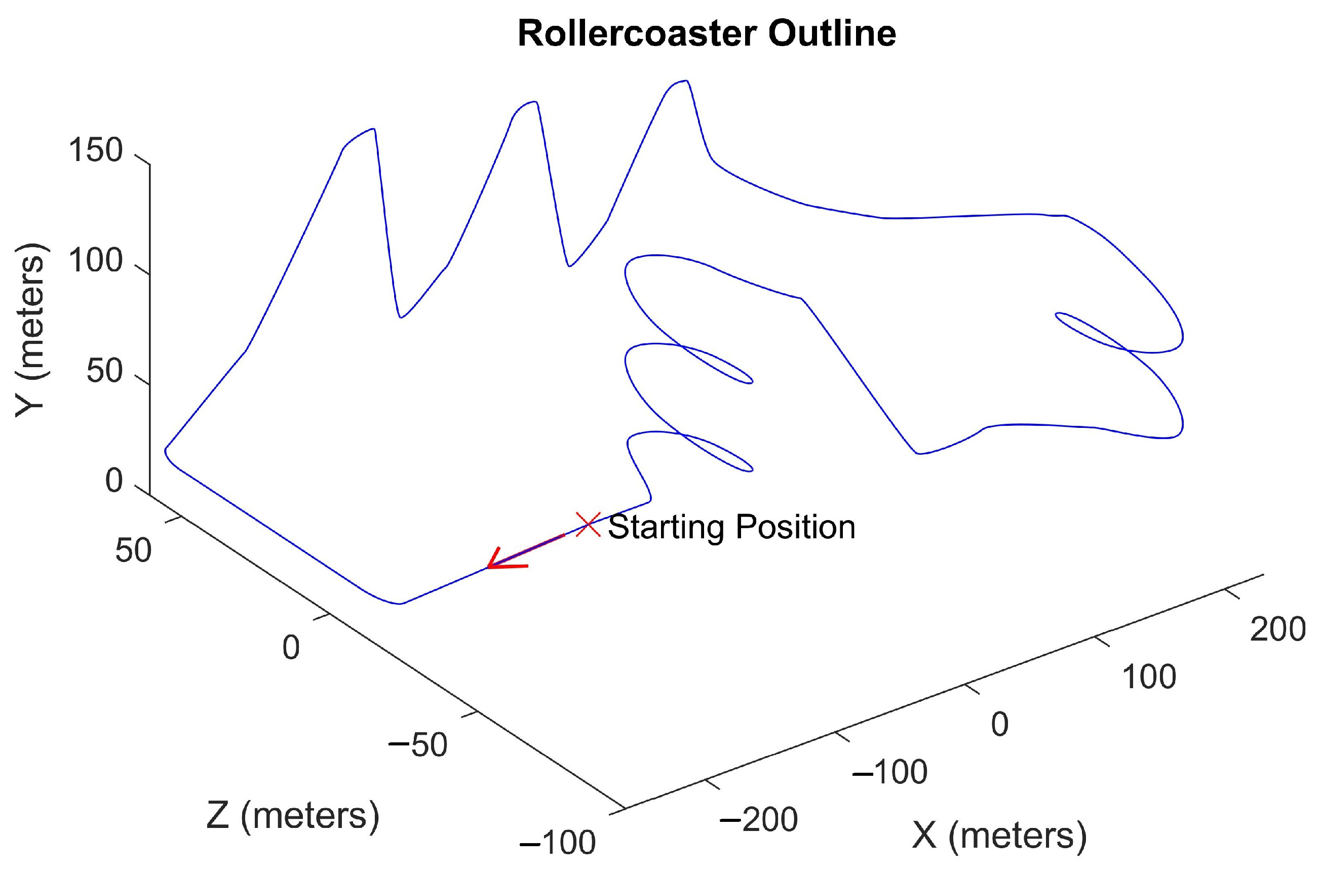
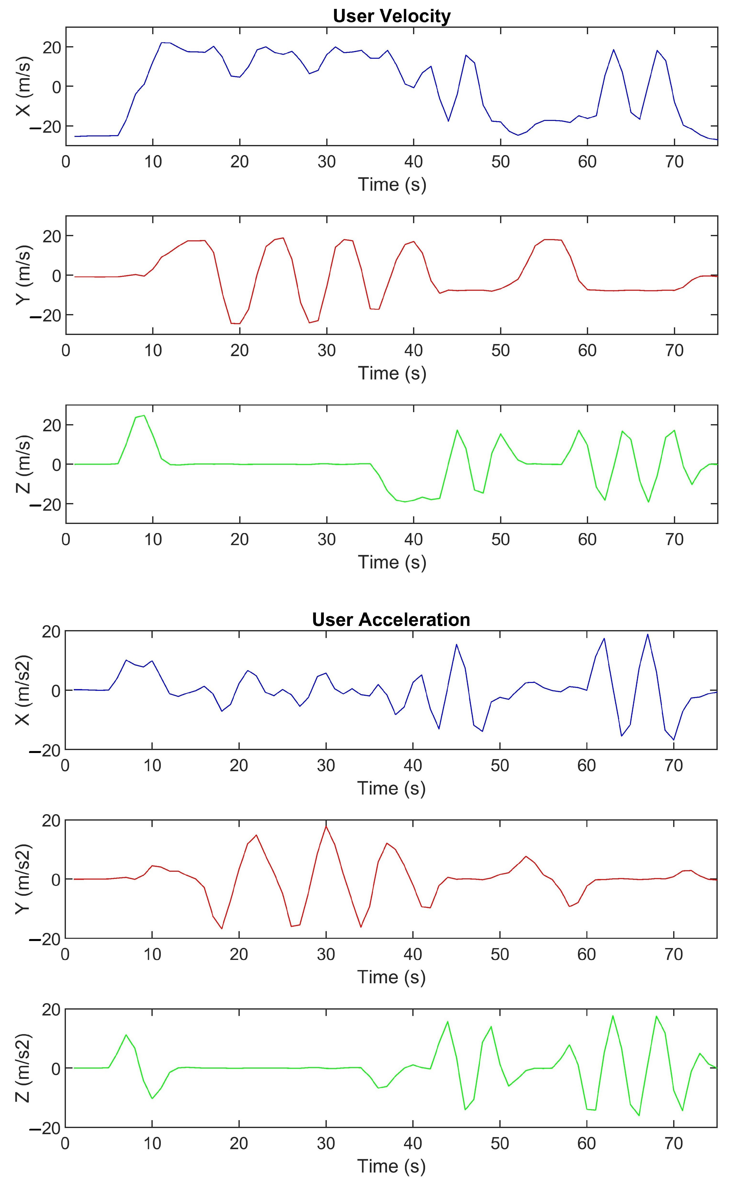
| Unity depth blur | HTC Vive Pro Eye | Rollercoaster | 26.9% |
| Foveated DoF (ours) | HTC Vive Pro Eye | Rollercoaster | 66.0% |
| User | NB | GC | FD | |||
|---|---|---|---|---|---|---|
| >200°/s | Peak | >200°/s | Peak | >200°/s | Peak | |
| AT | 106 | 810°/s | 89 | 502°/s | 59 | 354°/s |
| CT | 132 | 784°/s | 108 | 544°/s | 96 | 497°/s |
| EV | 88 | 859°/s | 99 | 743°/s | 74 | 556°/s |
| GB | 136 | 546°/s | 90 | 650°/s | 101 | 549°/s |
| HR | 115 | 773°/s | 125 | 663°/s | 97 | 568°/s |
| KK | 78 | 593°/s | 71 | 539°/s | 84 | 542°/s |
| LH | 132 | 731°/s | 93 | 707°/s | 103 | 581°/s |
| MB | 87 | 581°/s | 116 | 582°/s | 63 | 431°/s |
| MM | 112 | 703°/s | 95 | 697°/s | 88 | 553°/s |
| ND | 101 | 802°/s | 107 | 718°/s | 71 | 655°/s |
| NR | 86 | 824°/s | 119 | 702°/s | 105 | 603°/s |
| OQ | 88 | 595°/s | 92 | 629°/s | 95 | 612°/s |
| SA | 106 | 697°/s | 105 | 735°/s | 94 | 514°/s |
| SR | 97 | 710°/s | 82 | 657°/s | 68 | 570°/s |
| TB | 113 | 688°/s | 89 | 617°/s | 87 | 545°/s |
| UG | 115 | 591°/s | 84 | 623°/s | 89 | 511°/s |
| US | 92 | 597°/s | 111 | 502°/s | 89 | 533°/s |
| YK | 67 | 351°/s | 142 | 661°/s | 67 | 508°/s |
| Total | 1999 | 859°/s | 1923 | 743°/s | 1619 | 655°/s |
| System | Average Processing Time | 95% Confidence Interval | Frame Rate |
|---|---|---|---|
| NB | 15.9 ms | [15.9 ms, 15.9 ms] | 63 Hz |
| GC | 17.2 ms | [17.1 ms, 17.3 ms] | 58 Hz |
| FD | 16.7 ms | [16.6 ms, 16.8 ms] | 60 Hz |
Publisher’s Note: MDPI stays neutral with regard to jurisdictional claims in published maps and institutional affiliations. |
© 2021 by the authors. Licensee MDPI, Basel, Switzerland. This article is an open access article distributed under the terms and conditions of the Creative Commons Attribution (CC BY) license (https://creativecommons.org/licenses/by/4.0/).
Share and Cite
Hussain, R.; Chessa, M.; Solari, F. Mitigating Cybersickness in Virtual Reality Systems through Foveated Depth-of-Field Blur. Sensors 2021, 21, 4006. https://doi.org/10.3390/s21124006
Hussain R, Chessa M, Solari F. Mitigating Cybersickness in Virtual Reality Systems through Foveated Depth-of-Field Blur. Sensors. 2021; 21(12):4006. https://doi.org/10.3390/s21124006
Chicago/Turabian StyleHussain, Razeen, Manuela Chessa, and Fabio Solari. 2021. "Mitigating Cybersickness in Virtual Reality Systems through Foveated Depth-of-Field Blur" Sensors 21, no. 12: 4006. https://doi.org/10.3390/s21124006
APA StyleHussain, R., Chessa, M., & Solari, F. (2021). Mitigating Cybersickness in Virtual Reality Systems through Foveated Depth-of-Field Blur. Sensors, 21(12), 4006. https://doi.org/10.3390/s21124006