Abstract
The synthesis of four-bar linkage has been extensively researched, but for a long time, the problem of motion generation, path generation, and function generation have been studied separately, and their integration has not drawn much attention. This paper presents a numerical synthesis procedure for four-bar linkage that combines motion generation and function generation. The procedure is divided into two categories which are named as dependent combination and independent combination. Five feasible cases for dependent combination and two feasible cases for independent combination are analyzed. For each of feasible combinations, fully constrained vector loop equations of four-bar linkage are formulated in a complex plane. We present numerical examples to illustrate the synthesis procedure and determine the defect-free four-bar linkages.
1. Introduction
Linkage synthesis is to determine link dimensions of the linkage that achieves prescribed task positions [1,2,3,4]. Traditionally, linkage synthesis is divided into three types [5,6], motion generation, function generation, and path generation. Each of the synthesis types has been extensively researched and has many applications in various engineering fields, but, in some situations, a hybrid task needs to be performed. A hybrid task synthesis is to design the mechanisms that accomplish two or three of linkage synthesis types simultaneously, during a single movement. Many problems in engineering practice require some combination of these problem types. For example, the pick-and-place system requires a part not only to accomplish the picking task but also to avoid obstructions during a single movement [7], which is the problem of combination of motion and path generation for four-bar linkage. In automotive fields, stowing automotive seats frequently requires a combination of motion and function generation. The hybrid task synthesis can also be applied to aeronautic and astronautic fields and so on. In this paper, we present a numerical synthesis procedure for four-bar linkage that combines motion and function generation; this method can be extended and applied to six-bar and eight-bar linkages.
To the best of the author’s knowledge, the idea of hybrid task synthesis was proposed by Smaili and Diab [8] in 2006; they divided a crank cycle into several segments, each of the segments performed one of the synthesis types. In 2013, Tong and Murray [9] presented the synthesis for combination of motion generation and path generation, which differs from Ref. [8], the combination are satisfied in one segment. Based on the foundation, Brake et al. [10] studied the Alt–Burmester problems with all possible combinations, the Alt–Burmester problem is the combination of motion generation and path generation. In 2018, Zimmerman [11] presented a graphical method that tried to synthesize four-bar linkage to satisfy any combination of these three synthesis types. However, in the above literature, the combination of motion generation and function generation for four-bar linkage was not studied completely.
Generally, there are three linkage synthesis methods which are graphical method, optimization method and numerical analytical method. The graphical method is to draw the linkage step by step under geometric constraints by the target positions on the linkage through the poles and rotation angles. Beyer [12] shows a graphical method for two coupler points and specified input and output angle changes corresponding to those two points. Zimmerman [11] used Pole and rotation angle constraints to draw the four-bar linkage in a CAD software. The graphical method is intuitive, but the steps become extremely complex when the number of task positions increases. The optimization method is to obtain an optimum linkage by building an optimization model [8,13,14,15]. For linkage synthesis, only one linkage solution is obtained usually by an optimization method.
The numerical analytical method is to formulate the kinematic constraint loop equations and solve for the appropriate link lengths and pivot locations. The research for numerical analytical method of linkage belongs to the area, numerical algebraic geometry, which was proposed by Sommese and Wampler [16] in 1996. The foundation of numerical algebraic geometry is the solving of systems of polynomial equations based on the homotopy continuation method and to obtain all isolated solutions of the polynomial systems. Liu and McCarthy [4,17] applied a numerical analytical method to solve the problem of motion generation, and the number of task positions ranges from 2 to 5. Wampler et al. [18] used an analytical method to construct the constraint equation and solved it by a homotopy method for the nine point path synthesis problem for four-bar linkages, and they proved that the complete solution of the system are obtained. Plecnik and McCarthy [19,20] presented a numerical analytical method to synthesize function generation for six-bar linkages and solved it by the polynomial homotopy solver Bertini [21].
In this paper, we present a numerical synthesis procedure for four-bar linkage that combines motion generation and function generation, which was not addressed before. The procedure is divided into two categories which are named as dependent combination and independent combination. Five feasible cases for dependent combination and two feasible cases for independent combination are analyzed. For each of feasible combinations, fully constrained vector loop equations of four-bar linkage are formulated in complex planes. In addition, we give numerical examples to illustrate the numerical procedure and determine the defect-free linkages. In what follows, we present how to perform the numerical procedure.
1.1. Isotropic Coordinates
It is convenient to use vectors in complex plane to formulate constraint equations in planar kinematics [22]. Instead of denoting a vector as in a Cartesian coordinates system, we represent it as and its conjugate in complex plane, where , see Figure 1. Note that the length of vector can be calculated by . In addition, the unit vector is the rotation operation that defines the rotation from the fixed frame F to the reference frame . Applying the Euler identity, we have
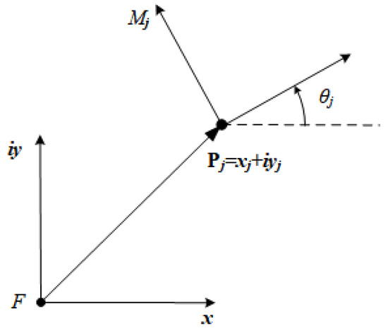
Figure 1.
Representation form of vector and rotation operation in a complex plane.
The conjugate of Equation (1) denotes the rotation from the reference frame to the fixed frame F, which is
1.2. Motion Generation
The task of motion generation is to guide the coupler link of a four-bar linkage through prescribed points and orientations. In this paper, we define the prescribed point and orientation as motion task position (MTP) which is denoted as , where is relative to the x-axis of the fixed frame F.
Figure 2 displays a four-bar linkage whose coupler link is passing through MTP from MTP . During the movement, input link rotates the angle of , output link rotates the angle of and coupler link rotates the angle of , which are relative to the position . We define and as rotation operations, so
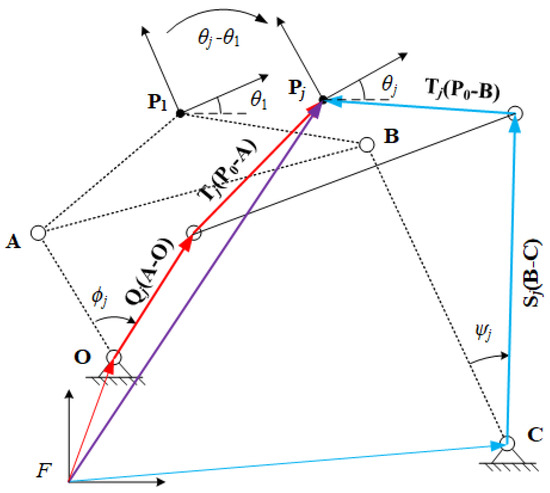
Figure 2.
Vector diagram of a four-bar linkage at MTP }.
The conjugates of Equation (3) denote reverse rotation with the same amount,
At MTP , the constraint vector loop equations of the four-bar linkage can be formulated by
The conjugate of Equation (5) are
Note that and are unit vectors, so they have the unit magnitude,
and can be expressed by solving Equation (5), and and by Equation (6). Then, substituting these expressions into Equation (7) to eliminated , and , ,
where , m denotes the maximum number of MTPs that a four-bar linkage can achieve during a movement. In Equation (8), , , and are specified by the designer, so there are eight unknowns, , , , , , , and . Note that and are two independent unknowns for solving the constraint loop equations, so are , , and . When , the number of equations is equal to the number of unknowns, which means the loop equations are fully constrained. This indicates a four-bar linkage can achieve at most five MTPs.
1.3. Function Generation
The task of function generation of four-bar linkage is to coordinate the rotation angles of input link and output link. In this paper, we define the position where the four-bar linkage is at and the linkage’s input angle is and output angle as function task position (FTP). FTP is denoted as , where the angles are relative to the x-axis of the fixed frame F.
Figure 3 displays a four-bar linkage is at FTP from FTP . During the movement, the input link rotates the angle of , the output links rotates the angle of , and the coupler link rotates the angle of , which are relative to the FTP . Thus, the corresponding rotations can be denoted as
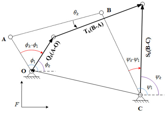
Figure 3.
Vector diagram of a four-bar linkage at FTP }.
The constraint loop equation for function generation can be formulated by
The conjugate of Equation (10) is
The unit vector has the unit magnitude,
and can be expressed by respective solving Equations (10) and (11), then substituting the expressions into Equation (12) to eliminate and ,
where , n represents the maximum number of FTPs that a four-bar linkage can achieve. Note that the fixed pivots of the four-bar linkage must be specified in advance to measure the angles of input and output for function generation. Thus, in Equation (13), , , , , , , and are specified by the designer. The unknowns are , , and . When , the loop equations are fully constrained; therefore, a four-bar linkage can achieve at most five FTPs.
2. The Synthesis of Mixed Generation
In Section 2, motion generation and function generation are synthesized separately, and a four-bar linkage can achieve at most five MTPs or five FTPs. In this section, we explore the relationship of combination between the number of MTPs and FTPs. Here, the mixed synthesis process is divided into two categories, dependent combination and independent combination. In what follows, we show how to synthesize and analyze these two types of mixed generation.
2.1. Dependent Combination
The task of mixed generation is also to determine the link dimensions of the four-bar linkage that achieves m MTPs and n FTPs during a period of movement. The dependent combination means that there is at least a common task position (CTP) that the linkage moves through a MTP and a FTP simultaneously. On the contrary, there is no CTP during the movement, which is called independent combination.
Let t denote the number of CTPs, and select one of CTPs as the first task position. For the rest of CTPs relative to the first task position, we have the constraints,
where the unknowns , , , , , , and denote the vectors and their conjugates of the four-bar linkage at the selected CTP. Here, , and . If , the Equation (14) always holds because , and .
According to Equation (8), the constraint equations for the rest of MTPs relative to the first task position are
where denote the coupler link rotations of the rest of MTPs relative to the selected CTP.
According to Equation (13), the constraint equations for the rest of FTPs relative to the first task position are
where and denote the input rotations and output rotations of the rest of FTPs relative to the selected CTP, respectively.
Combining Equations (14)–(16), there are eight unknowns, namely , , , , , , and . To satisfy that the mixed equations are fully constrained, the relationship between the number of unknowns and number of equations is
There are three cases for the value of t, which are , and . For case of , the combination of is equivalent to motion generation. The combinations and are feasible. Note that the combinations of and are infeasible because a four-bar linkage achieve at most FTPs, namely . For case of , there are two feasible combinations which are and . For case of , there is only a combination . The feasible dependent combinations of MTPs and FTPs are listed in Table 1.

Table 1.
Feasible dependent combinations of MTPs and FTPs.
2.1.1. The Case of
When , Equation (14) can be discarded. The mixed constraint equations are the combination of Equations (15) and (16) with the index or . Here, the mixed constraint equations are a polynomial equations system which includes eight equations and eight unknowns, and the degree of each equation is 2. According to Bezout theory [23], the upper limit of the number of the solution sets is . In kinematic synthesis, all isolated solution sets for the constraint equations should be obtained. In addition, the solutions should be checked to find those which can be formed as a four-bar linkage to achieve prescribed MTPs and FTPs in sequence and smoothly [24,25]. The constraint equations for the cases of can be solved by polynomial homotopy method to obtain all isolated solution sets.
2.1.2. The Case of
When , Equation (14) are linear equations, and , , , can be expressed by using , , , , which are
Substituting Equation (18) into Equations (15) and (16) can eliminate , , and , which decreases the number of unknowns to four. Now, , , , can be obtained by solving Equations (15) and (16). As there are only four unknowns, the equations system can be solved using a homotopy method or directly by the command in software. After the results of , , , are obtained, , , , and can be obtained easily by solving Equation (18).
2.1.3. The Case of
For case , only Equation (14) are applied. As all equations are linear, the conjugate equations can be omitted. Thus, the constraint equations are
It is easy to solve the equations to obtain the results of , , , because of the linear equations.
2.2. Independent Combination
The independence of mixed generation is a task to determine four-bar linkages that achieve m MTPs and n FTPs without any CTP during the movement, namely . Here, we select one of MTPs as the first MTP , and one of FTPs as the first FTP . In the four-bar linkage, , are fixed pivots, and , are moving pivots. Thus, we define the moving pivots at the first MTP as , , and at the first FTP as , .
For m MTPs, we have
For n FTPs, we have
To decrease the number of unknowns, we establish the relationship between , and , . In a complex plane, a unit vector can represent rotation operation; therefore, the rotation from the x-axis of the fixed frame to vectors and can be denoted, respectively, as
The rotation operations of input link and output link from the first MTP to first FTP can be denoted, respectively, as
Now, the relationship between , and , , and its conjugates are obtained,
3. Numerical Examples
In this section, we present numerical examples to illustrate the mixed constraint equations and determine non-defective four-bar linkages. For lack of space, we do not show numerical examples for all cases of mixed constraint equations. According to the number of unknowns in the nonlinear equations, we select one for maximum number of unknowns, the combination of , and one for minimum number of unknowns, the combination of , respectively.
3.1. Example for
For combination of , the four-bar linkage achieves 3 MTPs and 5 FTPs with a CTP. We specified the values and order of these positions in Table 2.
Table 2.
The prescribed MTPs and FTPs for .
In this example, the CTP is the fourth task position that the four-bar linkage passes through. substituting these values into Equations (15) and (16) to form a polynomial system with eight equations and eight unknowns. In order to obtain all isolated solution sets, [21,26] is applied to solve the polynomial system. To decrease the number of tracking path, here, we give a group division , and the multi-homogenious number [23,27] is 70. After 70 initial values are tracked, 60 solution sets are obtained. After checking the conjugates of and , 12 solution sets were remained. Then, filtering those which are defective linkages, a solution set is obtained which are
The images of the four-bar linkage moves through each of prescribed task positions of smoothly are displayed in Figure 4:
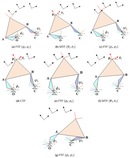
Figure 4.
The four-bar linkage moves through each of prescribed task positions of smoothly.
3.2. Example for
For combination of , the four-bar linkage achieve 3 MTPs and 3 FTPs, and each of MTPs and FTPs are passed through simultaneously. We specified the values and order of these task positions in Table 3.
Table 3.
The prescribed MTPs and FTPs for .
Substituting the values into Equation (19) can obtain a linear system which includes four equations and four unknowns. The solution set is
The images of the four-bar linkage move through each of prescribed task positions of smoothly are displayed in Figure 5.
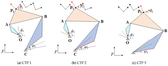
Figure 5.
The four-bar linkage moves through each of the prescribed task positions of , smoothly.
4. Conclusions
This paper presents a numerical procedure to synthesize four-bar linkage for mixed motion generation and function generation. The synthesis procedure is divided into two categories, dependent combination and independent combination. The feasible combinations are , , , , for dependent combination, and , for independent combination. Fully constrained vector loop equations for each of the feasible combinations are formulated and analyzed in a complex plane based on separate synthesis of motion and function generation. Numerical examples are presented to demonstrate the mixed synthesis procedure and determine defect-free four-bar linkages.
Author Contributions
Conceptualization, B.W., X.D. and X.L.; methodology, B.W. and X.L.; data investigation, B.W., X.D. and C.W.; analysis and validation, J.D., Y.D. and X.L.; writing–original draft, B.W.; writing–review and editing, B.W., C.W. and X.L. All authors have read and agreed to the published version of the manuscript.
Funding
This paper is supported by the State Key Laboratory of Robotics and Systems (HIT) under Grant No. SKLRS-2021-KF-01.
Institutional Review Board Statement
Not applicable.
Informed Consent Statement
Not applicable.
Data Availability Statement
No data available.
Conflicts of Interest
The authors declare no conflict of interest.
References
- Suh, C.H.; Radcliffe, C.W. Kinematics and Mechanism Design; John Wiley and Sons, Inc.: New York, NY, USA, 1978. [Google Scholar]
- Hunt, K.H. Kinematic Geometry of Mechanism; Oxford University Press: Oxford, MS, USA, 1978; Volume 7. [Google Scholar]
- Erdman, A.; Sandor, G.; Kota, S. Mechanism Design: Analysis and Synthesis, 4th ed.; Prentice-Hall, Inc.: Upper Saddle Rive, NJ, USA, 2001; Volume 1. [Google Scholar]
- McCarthy, J.M.; Soh, G.S. Geometric Design of Linkages, 2nd ed.; Springer: New York, NY, USA, 2010. [Google Scholar]
- Shiraz, K.H. Computer modelling and geometric construction for four-point synthesis of 4R spherical linkages. Appl. Math. Model. 2007, 31, 1874–1888. [Google Scholar] [CrossRef]
- Sun, J.; Chu, J.; Sun, B. A unified model of harmonic characteristic parameter method for dimensional synthesis of linkage mechanism. Appl. Math. Model. 2012, 36, 6001–6010. [Google Scholar]
- Kalpakjian, S.; Schmid, S. Manufacturing Engineering and Technology, 6th ed.; Prentice Hall, Inc.: Upper Saddle Rive, NJ, USA, 2009. [Google Scholar]
- Smaili, A.; Diab, N. Optimum synthesis of hybrid-task mechanisms using ant-gradient search method. Mech. Mach. Theory 2007, 42, 115–130. [Google Scholar] [CrossRef]
- Tong, Y.; Myszka, D.H.; Murray, A.P. Four-Bar Linkage Synthesis for a Combination of Motion and Path-Point Generation. In Proceedings of the ASME 2013 International Design Engineering Technical Conferences and Computers and Information in Engineering Conference, 37th Mechanisms and Robotics Conference, Portland, OR, USA, 4–7 August 2013; Volume 6A. [Google Scholar]
- Brake, D.A.; Hauenstein, J.D.; Murray, A.P.; Myszka, D.H.; Wampler, C.W. The Complete Solution of Alt–Burmester Synthesis Problems for Four-Bar Linkages. ASME J. Mech. Robot. 2016, 8, 142–149. [Google Scholar] [CrossRef]
- Zimmerman, R.A., II. Planar Linkage Synthesis for Mixed Motion, Path, and Function Generation Using Poles and Rotation Angles. ASME J. Mech. Robot. 2018, 10, 025004. [Google Scholar] [CrossRef]
- Beyer, R. The Kinematic Synthesis of Mechanisms; McGraw-Hill: New York, NY, USA, 2010; pp. 178–182. [Google Scholar]
- Smaili, A.; Diab, N. A New Approach to Shape Optimization for Closed Path Synthesis of Planar Mechanisms. ASME J. Mech. Des. 2007, 129, 941–948. [Google Scholar] [CrossRef]
- Acharyya, S.K.; Mandal, M. Performance of EAs for four-bar linkage synthesis. Mech. Mach. Theory 2009, 44, 1784–1794. [Google Scholar] [CrossRef]
- Liu, C.Y.; Yan, C.Q.; Wang, J.J. Performance of EAs for four-bar linkage synthesis. Ann. Nucl. Energy 2014, 64, 276–286. [Google Scholar] [CrossRef]
- Sommese, A.J.; Wampler, C.W. Numerical algebraic geometry. The Mathematics of Numerical Analysis (Park City, UT, 1995), 749–763. Lect. Appl. Math. 1996, 32. [Google Scholar]
- Liu, X.L.; Wang, C.; McCarhty, J.M. The design of coiling and uncoiling trusses using planar linkage modules. Mech. Mach. Theory 2020, 151, 103943. [Google Scholar] [CrossRef]
- Wampler, C.W.; Morgan, A.P.; Sommese, A.J. Complete Solution of the Nine-Point Path Synthesis Problem for Four-Bar Linkages. ASME J. Mech. Des. 1992, 114, 153–159. [Google Scholar] [CrossRef]
- Plecnik, M.M.; McCarthy, J.M. Computational Design of Stephenson II Six-Bar Function Generators for 11 Accuracy Points. ASME J. Mech. Robot. 2015, 8, 011017. [Google Scholar] [CrossRef]
- Plecnik, M.M.; McCarthy, J.M. Numerical Synthesis of Six-Bar Linkages for Mechanical Computation. ASME J. Mech. Robot. 2014, 6, 031012. [Google Scholar] [CrossRef]
- Bates, D.J.; Sommese, A.J.; Hauenstein, J.D.; Wampler, C.W. Numerically Solving Polynomial Systems with Bertini; SIAM: Philadelphia, PA, USA, 2013. [Google Scholar]
- Wampler, C.W. Isotropic coordinates, circularity, and Bezout numbers: Planar kinematics from a new perspective. In Proceedings of the ASME 1996 Design Engineering Technical Conferences and Computers in Engineering Conference, 24th Biennial Mechanisms Conference, Irvine, CA, USA, 18–22 August 1996; Volume 2A. [Google Scholar]
- Morgan, A.; Sommese, A. A homotopy for solving general polynomial systems that respects m-homogeneous structures. Appl. Math. Comput. 1987, 24, 101–113. [Google Scholar] [CrossRef]
- Chase, T.R.; Mirth, J.A. Circuits and branches of single degree-of-freedom planar linkages. ASME J. Mech. Des. 1993, 115, 223–230. [Google Scholar] [CrossRef]
- Mirth, J.A.; Chase, T.R. Circuit Rectification for Four Precision Position Synthesis of Stephenson Six-Bar Linkages. ASME J. Mech. Des. 2008, 46, 359–366. [Google Scholar] [CrossRef]
- Bates, D.J.; Hauenstein, J.D.; Sommese, A.J.; Wampler, C.W. Bertini: A Software Package for Numerical Algebraic Geometry. Bertini Home Page. 2013. Available online: https://bertini.nd.edu (accessed on 18 May 2021).
- Sommese, A.J.; Wampler, C.W. The Numerical Solution of Systems of Polynomials Arising in Engineering and Science; World Scientific: Hackensack, NJ, USA, 2005. [Google Scholar]
Publisher’s Note: MDPI stays neutral with regard to jurisdictional claims in published maps and institutional affiliations. |
© 2021 by the authors. Licensee MDPI, Basel, Switzerland. This article is an open access article distributed under the terms and conditions of the Creative Commons Attribution (CC BY) license (https://creativecommons.org/licenses/by/4.0/).