
A Visual and VAE Based Hierarchical Indoor Localization Method


Abstract
1. Introduction
- We designed a hierarchical localization framework that utilizes an unsupervised network VAE and SfM, which only requires RGB images as the input.
- We demonstrated that our proposed method can achieve 6DoF pose estimation and has higher localization accuracy than most deep learned methods.
2. Related Work
2.1. Visual-Based Localization
2.2. Variational Autoencoder
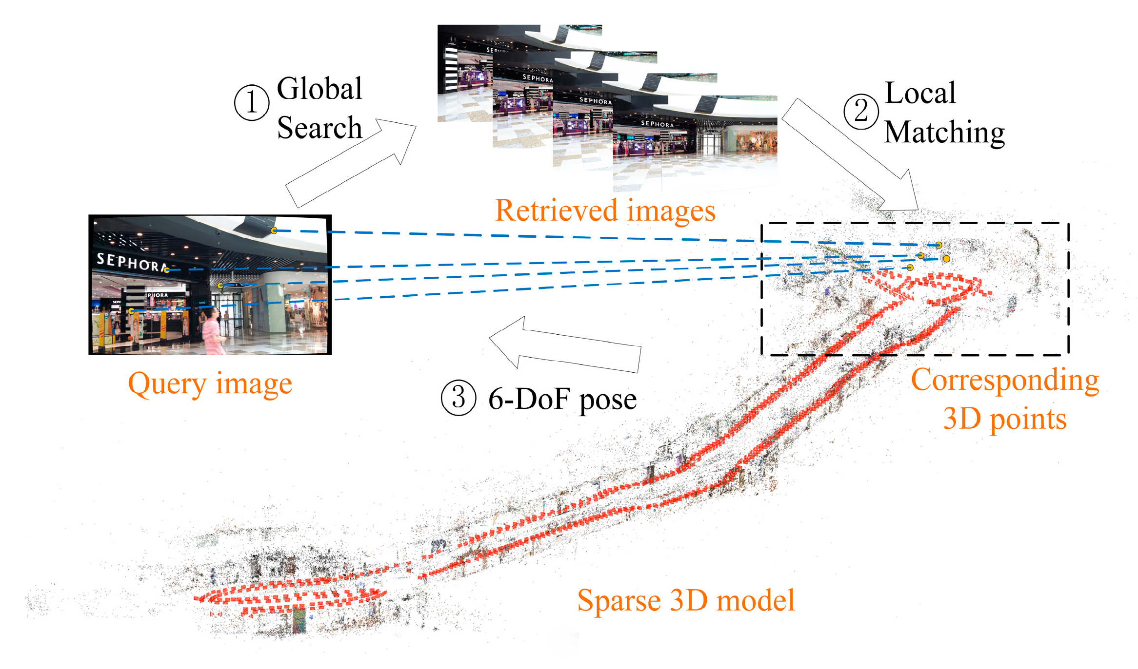
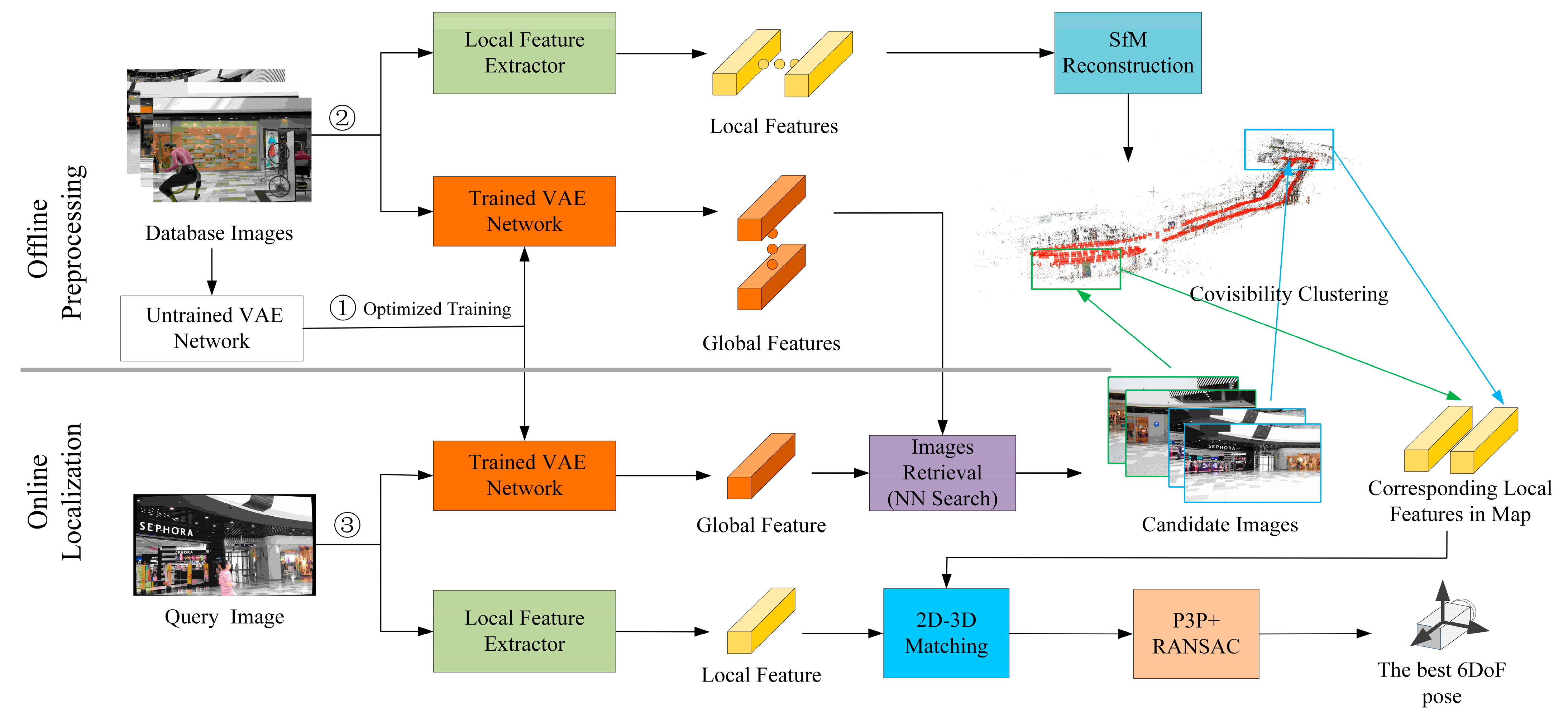
3. System Overview
4. Methods
4.1. Preprocessing
4.1.1. 3D Modeling
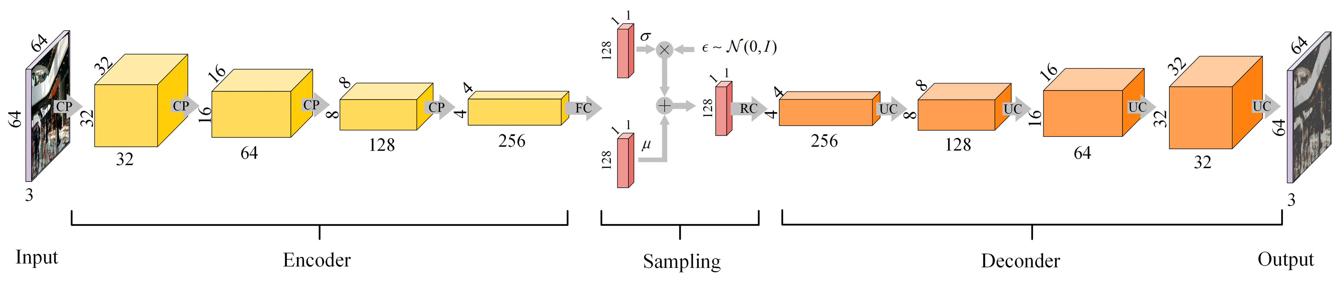
4.1.2. VAE Structure Design
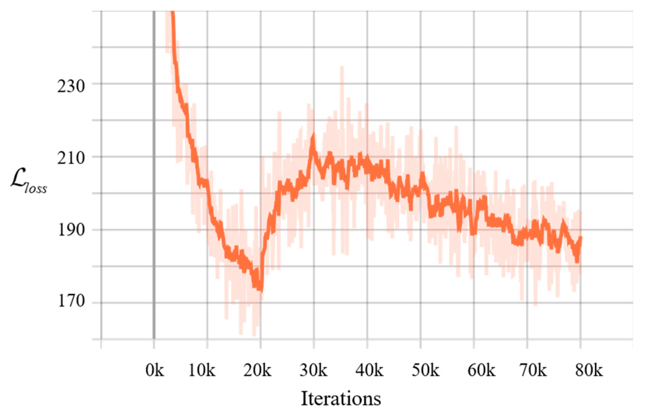
4.1.3. Training and Optimization
4.2. Localization
4.2.1. Prior Image Retrieval
4.2.2. Pose Estimation
5. Implementations and Evaluation
5.1. Implementations
5.2. Evaluation Results
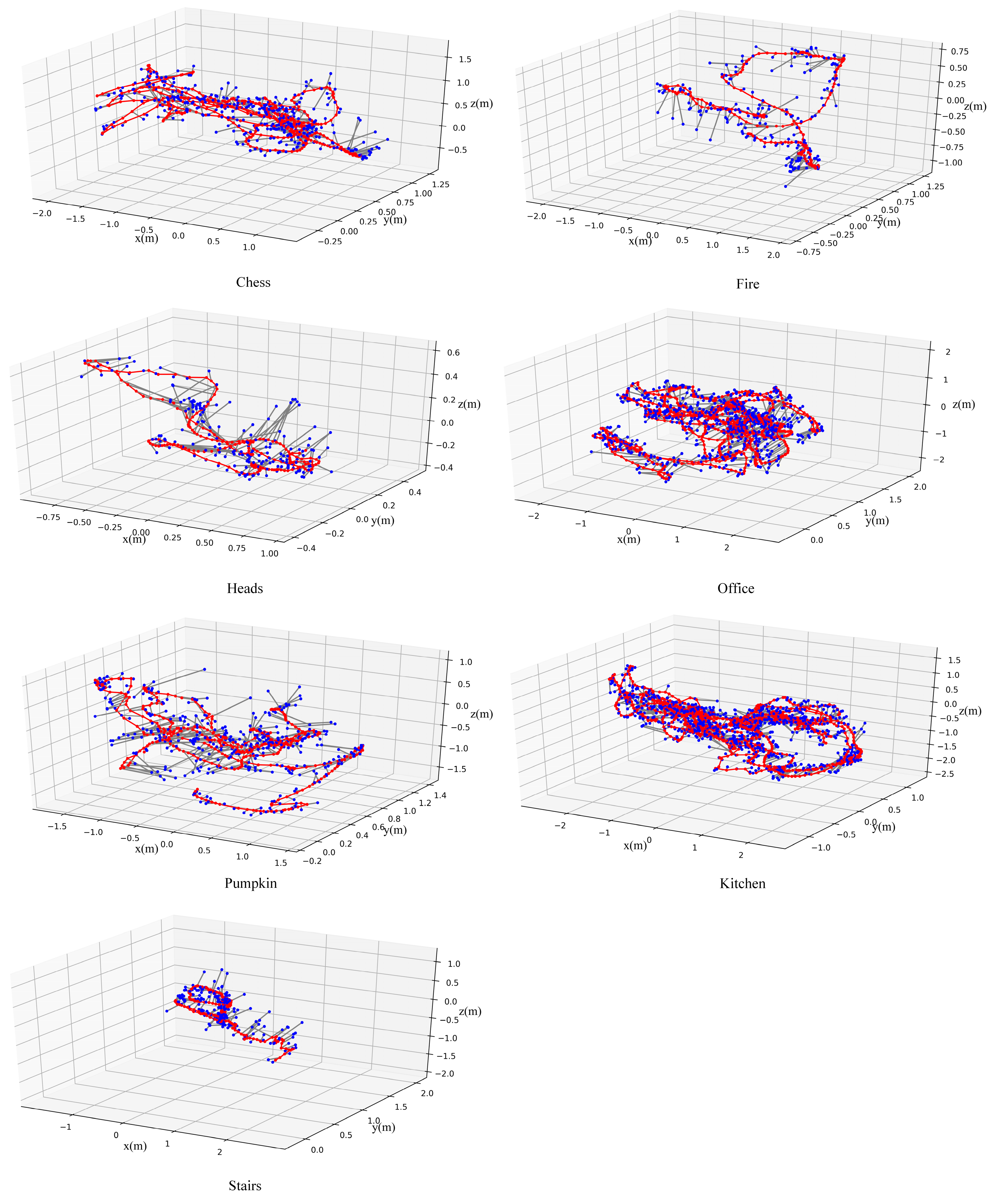
5.2.1. 7-Scenes Data Set
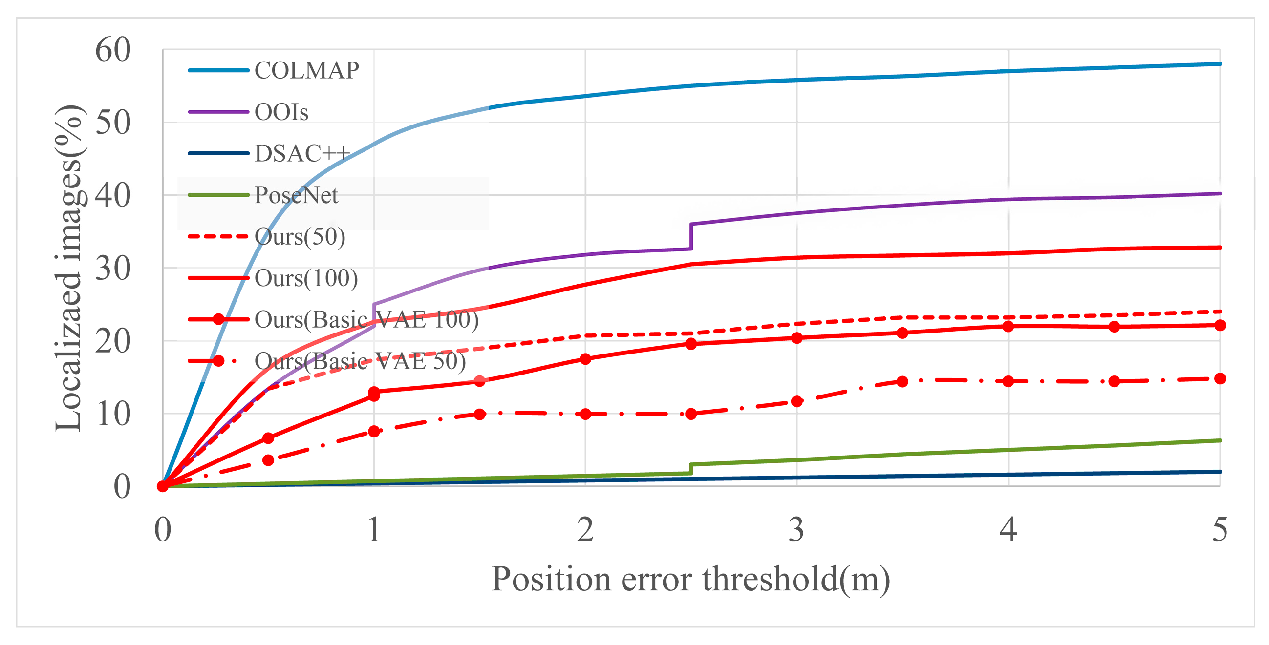
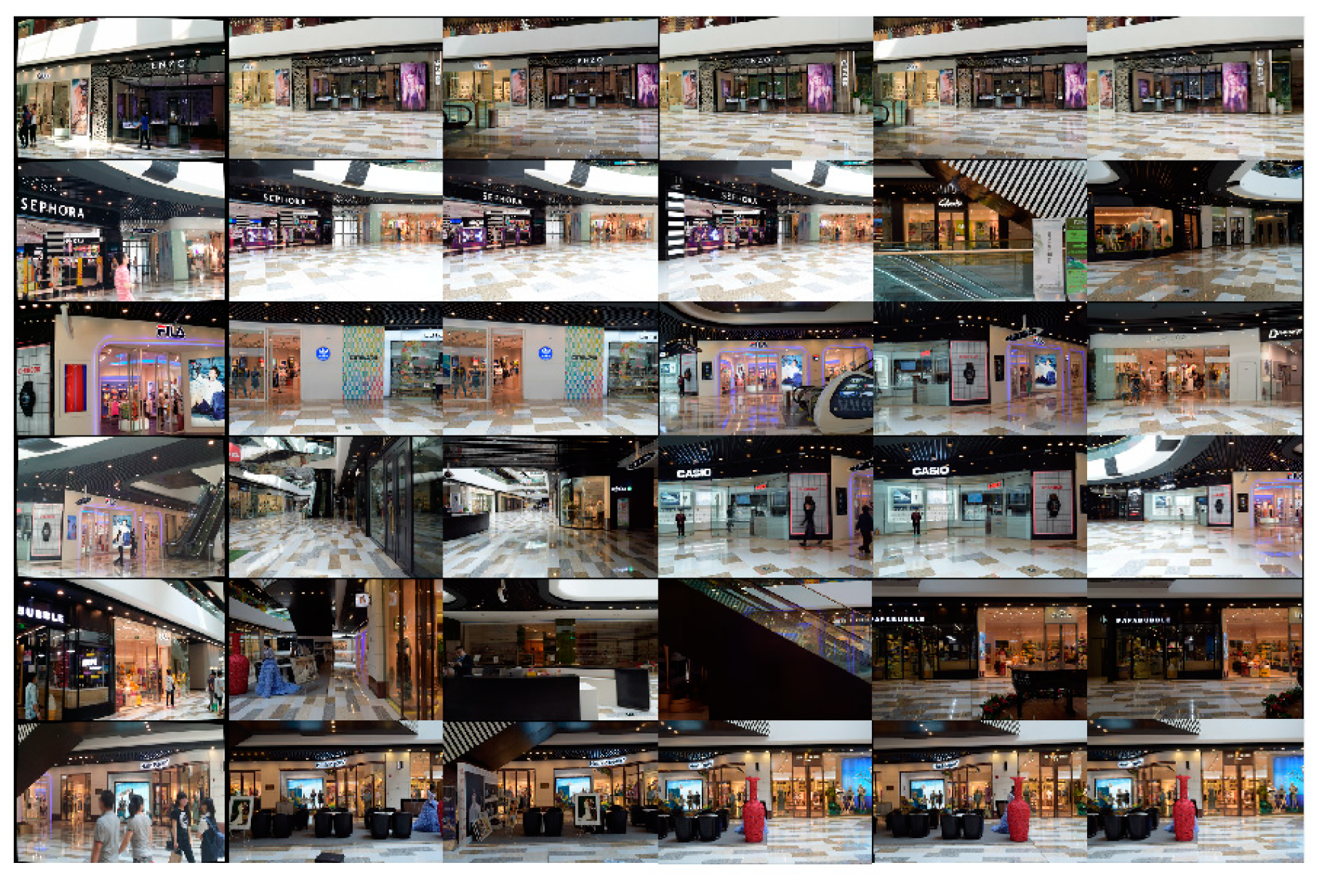
5.2.2. Baidu Data Set
6. Conclusions
Author Contributions
Funding
Institutional Review Board Statement
Informed Consent Statement
Acknowledgments
Conflicts of Interest
References
- Dong, J.; Noreikis, M.; Xiao, Y.; Ylä-Jääski, A. ViNav: A vision-based indoor navigation system for smartphones. Ieee Trans. Mob. Comput. 2018, 18, 1461–1475. [Google Scholar] [CrossRef]
- Bejuri, W.; Mohamad, M.M.; Zahilah, R.; Radzi, R.M. Emergency rescue localization (ERL) using GPS, wireless LAN and camera. Int. J. Softw Eng. Appl. 2015, 9, 217–232. [Google Scholar] [CrossRef][Green Version]
- Dickinson, P.; Cielniak, G.; Szymanezyk, O.; Mannion, M. Indoor positioning of shoppers using a network of Bluetooth Low Energy beacons. In Proceedings of the 2016 International Conference on Indoor Positioning and Indoor Navigation (IPIN), Alcala de Henares, Spain, 4–7 October 2016; IEEE: New York, NY, USA, 2016; pp. 1–8. [Google Scholar]
- Xia, S.; Liu, Y.; Yuan, G.; Zhu, M.; Wang, Z. Indoor fingerprint positioning based on Wi-Fi: An overview. Isprs Int. J. Geo-Inf. 2017, 6, 135. [Google Scholar] [CrossRef]
- Xiao, J.; Zhou, Z.; Yi, Y.; Ni, L.M. A survey on wireless indoor localization from the device perspective. Acm Comput. Surv. 2016, 49, 1–31. [Google Scholar] [CrossRef]
- Xu, H.; Ding, Y.; Li, P.; Wang, R.; Li, Y. An RFID indoor positioning algorithm based on Bayesian probability and K-nearest neighbor. Sensors 2017, 17, 1806. [Google Scholar] [CrossRef] [PubMed]
- Ramík, D.M.; Sabourin, C.; Moreno, R.; Madani, K. A machine learning based intelligent vision system for autonomous object detection and recognition. Appl. Intell. 2014, 40, 358–375. [Google Scholar] [CrossRef]
- Laskar, Z.; Melekhov, I.; Kalia, S.; Kannala, J. Camera Relocalization by Computing Pairwise Relative Poses Using Convolutional Neural Network. In Proceedings of the 2017 IEEE International Conference on Computer Vision Workshops (ICCVW), Venice, Italy, 22–29 October 2017; pp. 920–929. [Google Scholar]
- Engel, J.; Schöps, T.; Cremers, D. LSD-SLAM: Large-scale direct monocular SLAM. In European Conference on Computer Vision; Springer: Cham, Switzerland, 2014; pp. 834–849. [Google Scholar]
- Mur-Artal, R.; Montiel, J.M.M.; Tardos, J.D. ORB-SLAM: A versatile and accurate monocular SLAM system. Ieee Trans. Robot. 2015, 31, 1147–1163. [Google Scholar] [CrossRef]
- Schonberger, J.L.; Frahm, J.-M. Structure-from-motion revisited. In Proceedings of the IEEE Conference on Computer Vision and Pattern Recognition, Las Vegas, NV, USA, 27–30 June 2016; pp. 4104–4113. [Google Scholar]
- Taira, H.; Okutomi, M.; Sattler, T.; Cimpoi, M.; Pollefeys, M.; Sivic, J.; Pajdla, T.; Torii, A. InLoc: Indoor visual localization with dense matching and view synthesis. In Proceedings of the IEEE Conference on Computer Vision and Pattern Recognition, Salt Lake City, UT, USA, 18–23 June 2018; pp. 7199–7209. [Google Scholar]
- Sarlin, P.-E.; Debraine, F.; Dymczyk, M.; Siegwart, R.; Cadena, C. Leveraging deep visual descriptors for hierarchical efficient localization. In Proceedings of the Conference on Robot Learning, Zürich, Switzerland, 29–31 October 2018; pp. 456–465. [Google Scholar]
- Noh, H.; Araujo, A.; Sim, J.; Weyand, T.; Han, B. Large-scale image retrieval with attentive deep local features. In Proceedings of the IEEE international conference on computer vision, Venice, Italy, 22–29 October 2017; pp. 3456–3465. [Google Scholar]
- Revaud, J.; Almazán, J.; Rezende, R.S.; Souza, C.R.d. Learning with average precision: Training image retrieval with a listwise loss. In Proceedings of the IEEE/CVF International Conference on Computer Vision, Seoul, Korea, 27 October–2 November 2019; pp. 5107–5116. [Google Scholar]
- Sarlin, P.-E.; Cadena, C.; Siegwart, R.; Dymczyk, M. From coarse to fine: Robust hierarchical localization at large scale. In Proceedings of the IEEE/CVF Conference on Computer Vision and Pattern Recognition, Long Beach, CA, USA, 15–20 June 2019; pp. 12716–12725. [Google Scholar]
- Kendall, A.; Grimes, M.; Cipolla, R. Posenet: A convolutional network for real-time 6-dof camera relocalization. In Proceedings of the IEEE International Conference on Computer Vision, Santiago, Chile, 7–13 December 2015; pp. 2938–2946. [Google Scholar]
- Balntas, V.; Li, S.; Prisacariu, V. RelocNet: Continuous Metric Learning Relocalisation Using Neural Nets. In Proceedings of the European Conference on Computer Vision, Munich, Germany, 8–14 September 2018. [Google Scholar]
- Cimarelli, C.; Cazzato, D.; Olivares-Mendez, M.A.; Voos, H. Faster Visual-Based Localization with Mobile-PoseNet; Interdisciplinary Center for Security Reliability and Trust (SnT) University of Luxembourg: Luxembourg, 2019. [Google Scholar]
- Sattler, T.; Zhou, Q.; Pollefeys, M.; Leal-Taixe, L. Understanding the limitations of cnn-based absolute camera pose regression. In Proceedings of the IEEE Conference on Computer Vision and Pattern Recognition, Long Beach, CA, USA, 15–20 June 2019; pp. 3302–3312. [Google Scholar]
- Seifi, S.; Tuytelaars, T. How to Improve CNN-Based 6-DoF Camera Pose Estimation. In Proceedings of the 2019 IEEE/CVF International Conference on Computer Vision Workshop (ICCVW), Seoul, Korea, 27–28 October 2019. [Google Scholar]
- Wang, L.; Li, R.; Sun, J.; Seah, H.S.; Quah, C.K.; Zhao, L.; Tandianus, B. Image-similarity-based Convolutional Neural Network for Robot Visual Relocalization. Sens. Mater. 2020, 32, 1245–1259. [Google Scholar] [CrossRef]
- Schönberger, J.L.; Zheng, E.; Frahm, J.-M.; Pollefeys, M. Pixelwise view selection for unstructured multi-view stereo. In Proceedings of the European Conference on Computer Vision, Amsterdam, The Netherlands, 8–16 October 2016; Springer: Cham, Switzerland, 2016; pp. 501–518. [Google Scholar]
- Sattler, T.; Leibe, B.; Kobbelt, L. Efficient & effective prioritized matching for large-scale image-based localization. Ieee Trans. Pattern Anal. Mach. Intell. 2016, 39, 1744–1756. [Google Scholar]
- Brachmann, E.; Krull, A.; Nowozin, S.; Shotton, J.; Michel, F.; Gumhold, S.; Rother, C. Dsac-differentiable ransac for camera localization. In Proceedings of the IEEE Conference on Computer Vision and Pattern Recognition, Honolulu, HI, USA, 21–26 July 2017; pp. 6684–6692. [Google Scholar]
- Brachmann, E.; Rother, C. Learning Less is More—6D Camera Localization via 3D Surface Regression. In Proceedings of the Computer Vision and Pattern Recognition, Salt Lake City, UT, USA, 18–22 June 2018; pp. 4654–4662. [Google Scholar]
- Meng, L.; Chen, J.; Tung, F.; Little, J.J.; Valentin, J.; de Silva, C.W. Backtracking regression forests for accurate camera relocalization. In Proceedings of the 2017 IEEE/RSJ International Conference on Intelligent Robots and Systems (IROS), Vancouver, BC, Canada, 24–28 September 2017; IEEE: New York, NY, USA, 2017; pp. 6886–6893. [Google Scholar]
- Nister, D.; Stewenius, H. Scalable recognition with a vocabulary tree. In Proceedings of the 2006 IEEE Computer Society Conference on Computer Vision and Pattern Recognition (CVPR’06), New York, NY, USA, 17–22 June 2006; pp. 2161–2168. [Google Scholar]
- Li, Y.; Snavely, N.; Huttenlocher, D.P. Location recognition using prioritized feature matching. In Proceedings of the European Conference on Computer Vision, Heraklion, Crete, 5–11 September 2010; Springer: Cham, Switzerland, 2015; pp. 791–804. [Google Scholar]
- Middelberg, S.; Sattler, T.; Untzelmann, O.; Kobbelt, L. Scalable 6-dof localization on mobile devices. In Proceedings of the European Conference on Computer Vision, Zurich, Switzerland, 6–12 September 2014; Springer: Cham, Switzerland, 2014; pp. 268–283. [Google Scholar]
- Lowe, D.G. Distinctive image features from scale-invariant keypoints. Int. J. Comput. Vis. 2004, 60, 91–110. [Google Scholar] [CrossRef]
- Gálvez-López, D.; Tardos, J.D. Bags of binary words for fast place recognition in image sequences. Ieee Trans. Robot. 2012, 28, 1188–1197. [Google Scholar] [CrossRef]
- Jégou, H.; Douze, M.; Schmid, C.; Pérez, P. Aggregating local descriptors into a compact image representation. In Proceedings of the 2010 IEEE Computer Society Conference on Computer Vision and Pattern Recognition, San Francisco, CA, USA, 13–18 June 2010; pp. 3304–3311. [Google Scholar]
- Torii, A.; Arandjelovic, R.; Sivic, J.; Okutomi, M.; Pajdla, T. 24/7 place recognition by view synthesis. In Proceedings of the IEEE Conference on Computer Vision and Pattern Recognition, Boston, MA, USA, 7–12 June 2015; pp. 1808–1817. [Google Scholar]
- Zheng, L.; Yang, Y.; Tian, Q. SIFT meets CNN: A decade survey of instance retrieval. Ieee Trans. Pattern Anal. Mach. Intell. 2017, 40, 1224–1244. [Google Scholar] [CrossRef] [PubMed]
- Chen, W.; Liu, Y.; Wang, W.; Bakker, E.; Georgiou, T.; Fieguth, P.; Liu, L.; Lew, M.S. Deep Image Retrieval: A Survey. arXiv 2021, arXiv:2101.11282. [Google Scholar]
- Arandjelovic, R.; Gronat, P.; Torii, A.; Pajdla, T.; Sivic, J. NetVLAD: CNN architecture for weakly supervised place recognition. In Proceedings of the IEEE Conference on Computer Vision and Pattern Recognition, Las Vegas, NV, USA, 27–30 June 2016; pp. 5297–5307. [Google Scholar]
- Torii, A.; Taira, H.; Sivic, J.; Pollefeys, M.; Okutomi, M.; Pajdla, T.; Sattler, T. Are large-scale 3d models really necessary for accurate visual localization? In Proceedings of the IEEE Conference on Computer Vision and Pattern Recognition, Honolulu, HI, USA, 21–26 July 2017; pp. 1637–1646. [Google Scholar]
- Camposeco, F.; Cohen, A.; Pollefeys, M.; Sattler, T. Hybrid camera pose estimation. In Proceedings of the IEEE Conference on Computer Vision and Pattern Recognition, Salt Lake City, UT, USA, 18–23 June 2018; pp. 136–144. [Google Scholar]
- Sarlin, P.-E.; Debraine, F.; Dymczyk, M.; Siegwart, R.; Cadena, C. Leveraging deep visual descriptors for hierarchical efficient localization. arXiv 2018, arXiv:1809.01019. [Google Scholar]
- Hinton, G.; Vinyals, O.; Dean, J. Distilling the knowledge in a neural network. arXiv 2015, arXiv:1503.02531. [Google Scholar]
- Kingma, D.P.; Welling, M. Auto-encoding variational bayes. arXiv 2013, arXiv:1312.6114. [Google Scholar]
- Kingma, D.P.; Welling, M. An Introduction to Variational Autoencoders. Found. Trends® Mach. Learn. 2019, 12, 307–392. [Google Scholar] [CrossRef]
- Lucas, J.; Tucker, G.; Grosse, R.; Norouzi, M. Understanding posterior collapse in generative latent variable models. In Proceedings of the 2019 Deep Generative Models for Highly Structured Data, New Orleans, LA, USA, 6 May 2019. [Google Scholar]
- Wu, H.; Fieri, M. Learning product codebooks using vector-quantized autoencoders for image retrieval. In Proceedings of the 7th IEEE Global Conference on Signal and Information Processing, GlobalSIP 2019, Ottawa, ON, Canada, 11–14 November 2019; Institute of Electrical and Electronics Engineers Inc.: Piscataway, NJ, USA, 2019. [Google Scholar]
- Li, X.; Chen, Z.; Poon, L.K.; Zhang, N.L. Learning latent superstructures in variational autoencoders for deep multidimensional clustering. arXiv 2018, arXiv:1803.05206. [Google Scholar]
- Jiang, Z.; Zheng, Y.; Tan, H.; Tang, B.; Zhou, H. Variational deep embedding: An unsupervised and generative approach to clustering. arXiv 2016, arXiv:1611.05148. [Google Scholar]
- Schönberger, J.L.; Pollefeys, M.; Geiger, A.; Sattler, T. Semantic visual localization. In Proceedings of the IEEE Conference on Computer Vision and Pattern Recognition, Salt Lake City, UT, USA, 18–23 June 2018; pp. 6896–6906. [Google Scholar]
- Asperti, A.; Trentin, M. Balancing reconstruction error and Kullback-Leibler divergence in Variational Autoencoders. IEEE Access 2020, 8, 199440–199448. [Google Scholar] [CrossRef]
- Bowman, S.R.; Vilnis, L.; Vinyals, O.; Dai, A.M.; Jozefowicz, R.; Bengio, S. Generating sentences from a continuous space. arXiv 2015, arXiv:1511.06349. [Google Scholar]
- Kingma, D.P.; Salimans, T.; Jozefowicz, R.; Chen, X.; Sutskever, I.; Welling, M. Improving variational inference with inverse autoregressive flow.(nips). arXiv 2016, arXiv:1606.04934. [Google Scholar]
- Shotton, J.; Glocker, B.; Zach, C.; Izadi, S.; Criminisi, A.; Fitzgibbon, A. Scene coordinate regression forests for camera relocalization in RGB-D images. In Proceedings of the IEEE Conference on Computer Vision and Pattern Recognition, Portland, OR, USA, 23–28 June 2013; pp. 2930–2937. [Google Scholar]
- Sun, X.; Xie, Y.; Luo, P.; Wang, L. A dataset for benchmarking image-based localization. In Proceedings of the IEEE Conference on Computer Vision and Pattern Recognition, Honolulu, HI, USA, 21–26 July 2017; pp. 7436–7444. [Google Scholar]
- Kingma, D.P.; Ba, J. Adam: A method for stochastic optimization. arXiv 2014, arXiv:1412.6980. [Google Scholar]
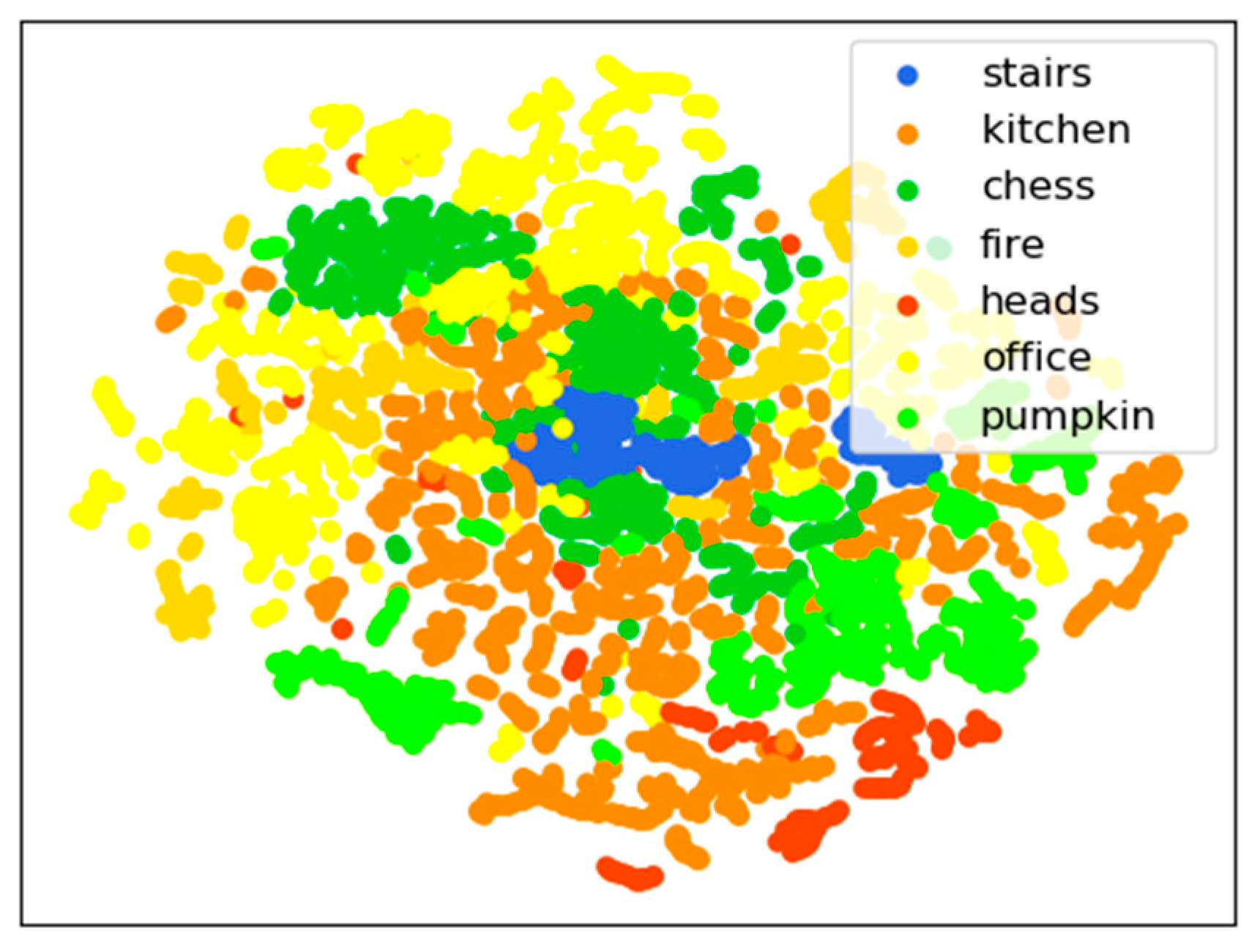
- Der Maaten, L.V.; Hinton, G.E. Visualizing data using t-SNE. J. Mach. Learn. Res. 2008, 9, 2579–2605. [Google Scholar]
- Weinzaepfel, P.; Csurka, G.; Cabon, Y.; Humenberger, M. Visual Localization by Learning Objects-Of-Interest Dense Match Regression. In Proceedings of the Computer Vision and Pattern Recognition, Long Beach, CA, USA, 16–20 June 2019; pp. 5634–5643. [Google Scholar]


| Data Sets | 7-Scenes Data Set | Baidu Data Set | |
|---|---|---|---|
| Parameters | |||
| Training images resolution (pixel) | 640 × 480 | 2992 × 2000 | |
| Testing images resolution (pixel) | 640 × 480 | 2064 × 1161, 1632 × 1224 2104 × 1560, 2104 × 1184 | |
| Downsize resolution (pixel) | 64 × 64 × 3 | 128 × 96 × 3 | |
| Input size of VAE (pixel) | 64 × 64 × 3 | Cropped into four corners and a center with a size of 64 × 64 × 3 (5 images) | |
| Dimension of global descriptor (dimension) | 128 | 640 | |
| Batch size | 50 | 50 | |
| learning rate | 1 × 10⁻⁴ | 1 × 10⁻⁴ | |
| 1 | 1 | ||
| KL annealing beginning Moment (iteration) | 20 k | 20 k | |
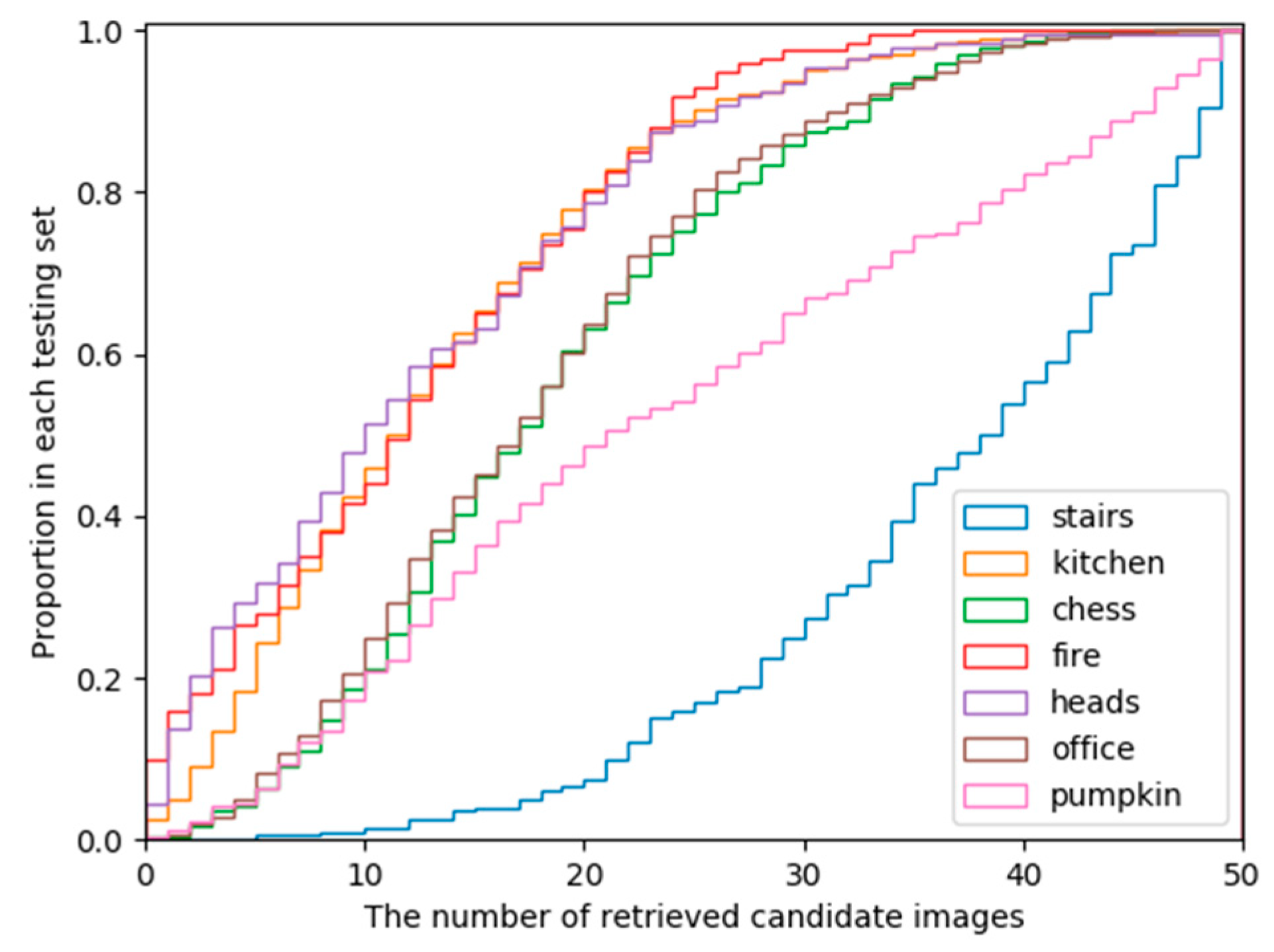
| Number of retrieved images | 50 | 50 (or 100) | |
| P3P-RANSAC reprojection error (pixel) | 10 | 10 | |
| Methods | Relative PN [18] | RelocNet [19] | Dense-VLAD [35] | Mobile-PoseNet [20] | Improved CNN-Based Pose Estimation [22] | Image-Similarity-Based Method [23] | Ours (Basic VAE, 50) | Ours (50) | |
|---|---|---|---|---|---|---|---|---|---|
| Data Sets | |||||||||
| Chess | 0.13/6.46 | 0.12/4.14 | 0.21/12.5 | 0.17/6.78 | 0.17/5.34 | 0.21/5.73 | 0.42/7.25 | 0.12/2.32 | |
| Fire | 0.26/12.7 | 0.26/10.4 | 0.33/13.8 | 0.36/13.0 | 0.30/10.36 | 0.40/12.11 | 0.55/8.72 | 0.15/3.07 | |
| Heads | 0.14/12.3 | 0.14/10.5 | 0.15/14.9 | 0.19/15.3 | 0.15/11.73 | 0.25/14.38 | 0.44/10.26 | 0.11/3.64 | |
| Offices | 0.21/7.35 | 0.18/5.32 | 0.28/11.2 | 0.26/8.50 | 0.27/7.10 | 0.30/7.58 | 0.53/8.57 | 0.16/2.54 | |
| Pumpkin | 0.24/6.35 | 0.26/4.17 | 0.31/11.3 | 0.31/7.53 | 0.23/5.83 | 0.37/7.46 | 0.59/9.38 | 0.16/2.33 | |
| Kitchen | 0.24/8.03 | 0.23/5.08 | 0.30/12.3 | 0.33/7.72 | 0.29/ 6.95 | 0.42/7.11 | 0.55/8.65 | 0.14/2.37 | |
| Stairs | 0.27/11.8 | 0.28/7.53 | 0.25/15.8 | 0.41/13.6 | 0.30/8.30 | 0.36/11.82 | 0.62/12.53 | 0.16/2.34 | |
| Processes | Global Search | Covisibility Clustering | Feature Match | P3P-RANSAC | Total | |
|---|---|---|---|---|---|---|
| Methods | ||||||
| Ours (50) | 0.12 | 0.07 | 0.98 | 1.53 | 2.70 | |
| Ours (Basic VAE, 50) | 0.12 | 0.07 | 0.98 | 1.53 | 2.70 | |
| Ours (100) | 0.24 | 0.14 | 2.26 | 1.49 | 4.13 | |
| Ours (Basic VAE, 100) | 0.24 | 0.14 | 2.26 | 1.49 | 4.13 | |
| COLMAP | 47.61 | |||||
Publisher’s Note: MDPI stays neutral with regard to jurisdictional claims in published maps and institutional affiliations. |
© 2021 by the authors. Licensee MDPI, Basel, Switzerland. This article is an open access article distributed under the terms and conditions of the Creative Commons Attribution (CC BY) license (https://creativecommons.org/licenses/by/4.0/).
Share and Cite
Jiang, J.; Zou, Y.; Chen, L.; Fang, Y. A Visual and VAE Based Hierarchical Indoor Localization Method. Sensors 2021, 21, 3406. https://doi.org/10.3390/s21103406
Jiang J, Zou Y, Chen L, Fang Y. A Visual and VAE Based Hierarchical Indoor Localization Method. Sensors. 2021; 21(10):3406. https://doi.org/10.3390/s21103406
Chicago/Turabian StyleJiang, Jie, Yin Zou, Lidong Chen, and Yujie Fang. 2021. "A Visual and VAE Based Hierarchical Indoor Localization Method" Sensors 21, no. 10: 3406. https://doi.org/10.3390/s21103406
APA StyleJiang, J., Zou, Y., Chen, L., & Fang, Y. (2021). A Visual and VAE Based Hierarchical Indoor Localization Method. Sensors, 21(10), 3406. https://doi.org/10.3390/s21103406