Author Contributions
Conceptualization, R.D.C. and N.C.Y.; Data curation, R.D.C. and N.C.Y.; Funding acquisition, N.C.Y.; Investigation, R.D.C. and N.C.Y.; Methodology, R.D.C. and N.C.Y.; Project administration, N.C.Y.; Software, R.D.C. and N.C.Y.; Validation, N.C.Y.; Visualization, R.D.C.; Writing—original draft, R.D.C.; Writing—review & editing, N.C.Y. All authors have read and agreed to the published version of the manuscript.
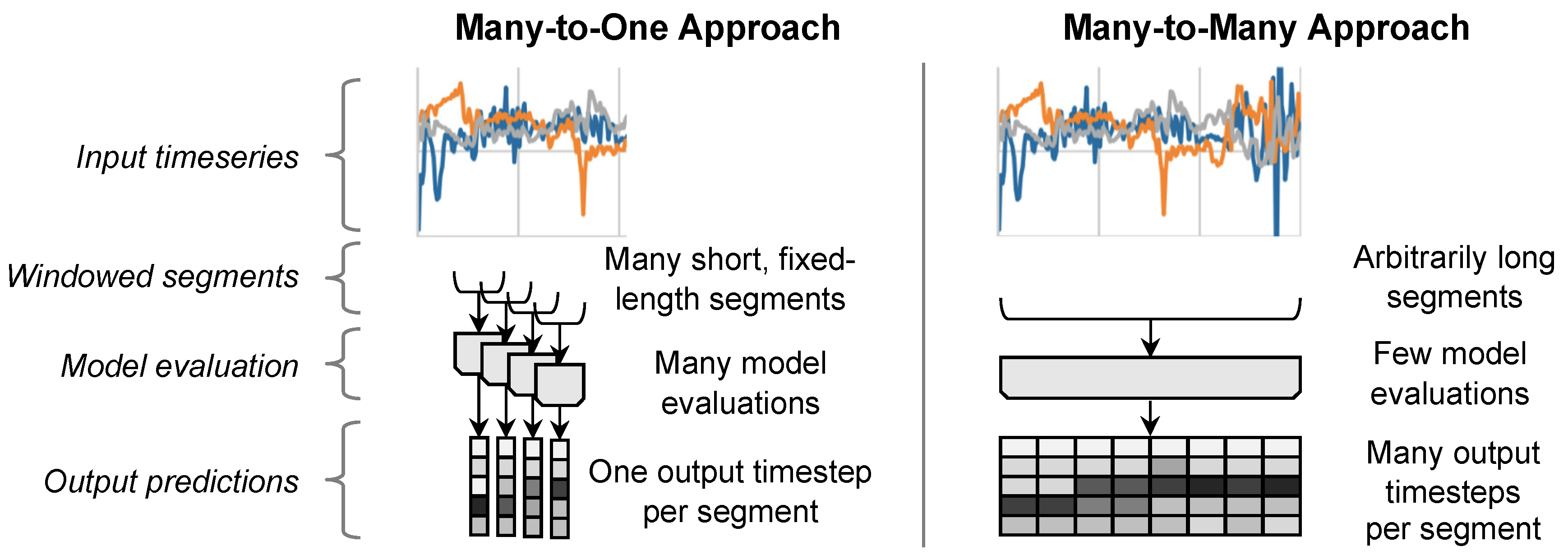
Figure 1.
In a typical many-to-one approach (left) an input is first divided into fixed-length overlapping windows, then a model processes each window individually, generating a class prediction for each one, and finally the predictions are concatenated into an output time series. In a many-to-many approach (right), the entire output time series is generated with a single model evaluation.
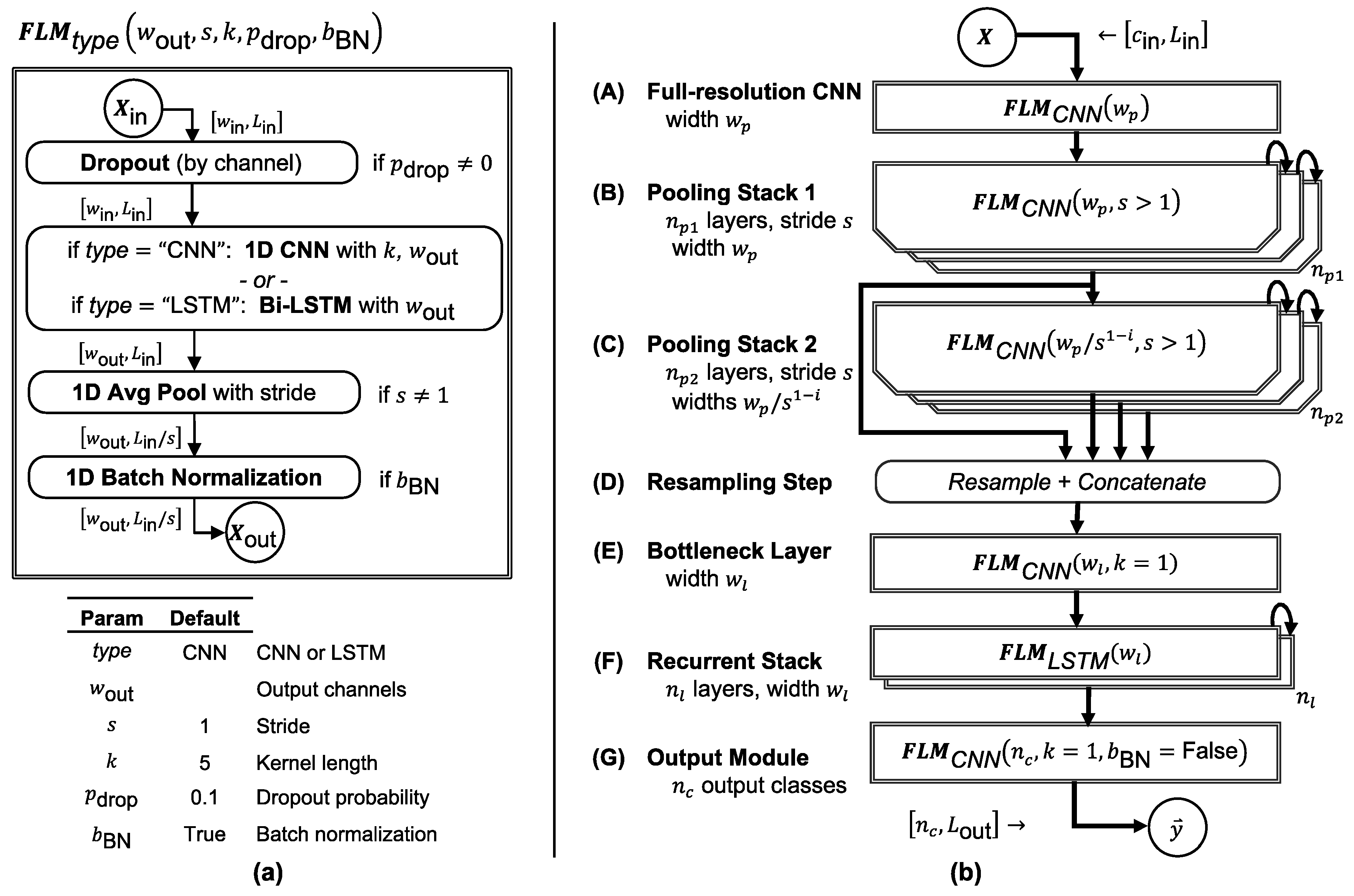
Figure 2.
FilterNet architecture. (a) Each FilterNet model is composed primarily of one or more stacks of FilterNet layer modules (FLMs), which are parameterized and constructed as shown (see text for elaboration). (b) In the prototypical FilterNet component architecture, FLMs are grouped into components that can be parameterized and combined to implement time series classifiers of varying speed and complexity, tuned to the problem at hand.
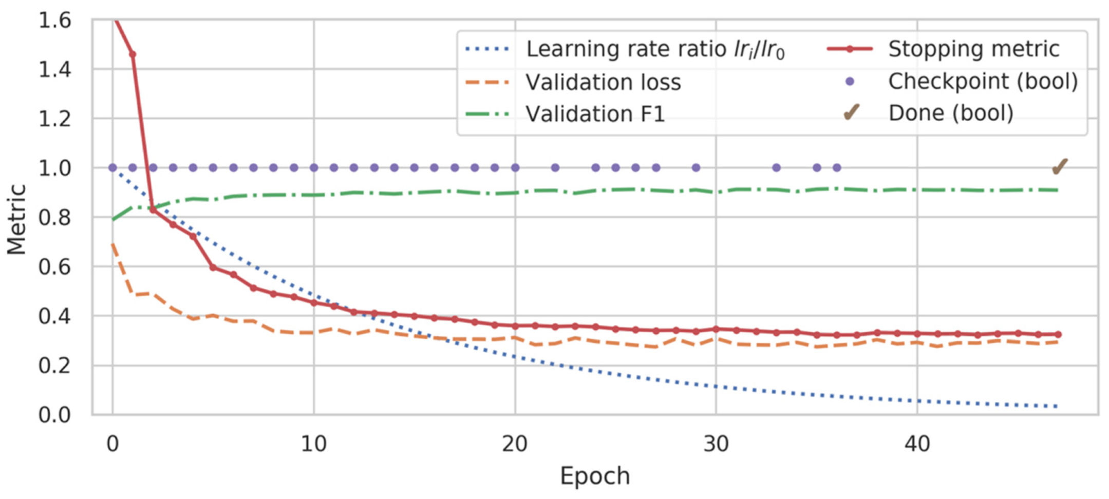
Figure 3.
Representative training history for a ms-C/L model. While the validation loss oscillated and had near-global minima at epochs 27, 35, and 41, the custom stopping metric (see text) adjusted more predictably to a minimum at epoch 36. Training was stopped at epoch 47 and the model from epoch 36 was restored and used for subsequent inference.
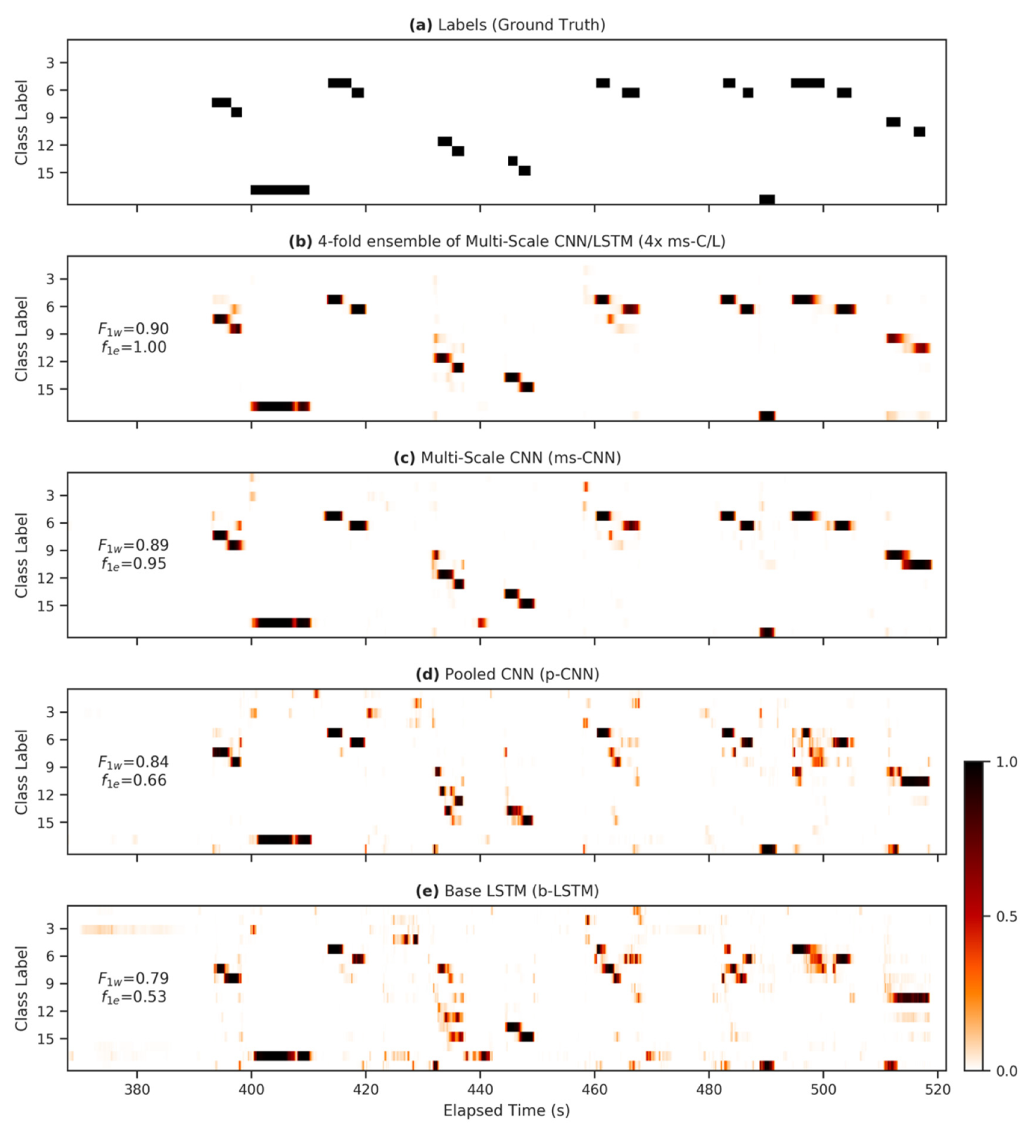
Figure 4.
Heatmap demonstrating differences between model outputs. (a) The ground-truth labels for 150 s during the first run in the standard Opportunity test set; (b–e) alongside the corresponding predictions for the 17 non-null behavior classes for various FilterNet architectures. Panes are annotated with weighted F1 scores ( and the event-based ) calculated over the plotted region.
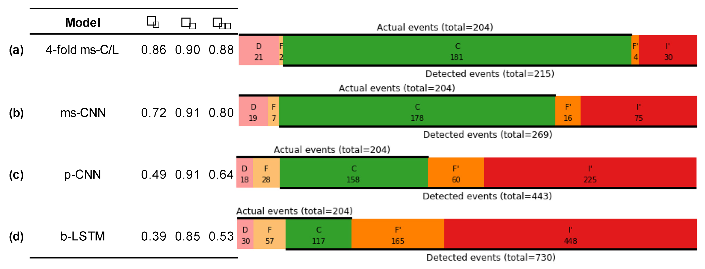
Figure 5.
Event-based metrics. Performance metrics for several classifiers, including event-based precision , recall , and F1 score , alongside event summary diagrams, each for a single representative run.
Figure 5.
Event-based metrics. Performance metrics for several classifiers, including event-based precision , recall , and F1 score , alongside event summary diagrams, each for a single representative run.
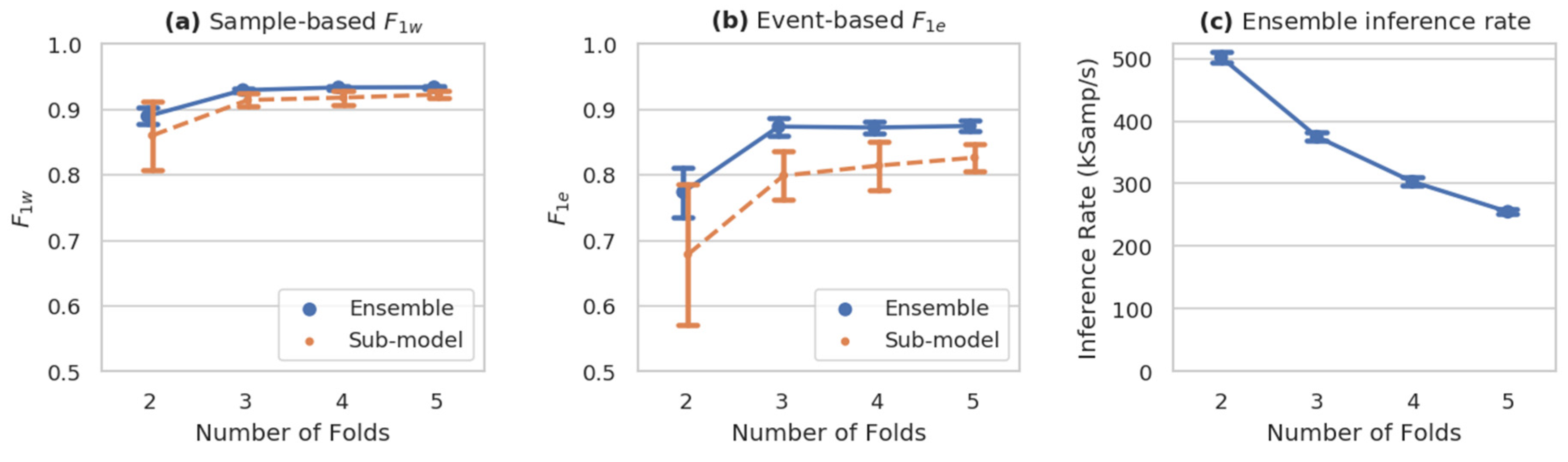
Figure 6.
Performance of n-fold ensembled ms-C/L models. Both sample-based (a) and event-based (b) weighted F1 metrics improve substantially with the number of ensembled models, plateauing between 3–5 folds, while inference rate (pane c) decreases. (mean sd, n = 10).
Figure 6.
Performance of n-fold ensembled ms-C/L models. Both sample-based (a) and event-based (b) weighted F1 metrics improve substantially with the number of ensembled models, plateauing between 3–5 folds, while inference rate (pane c) decreases. (mean sd, n = 10).
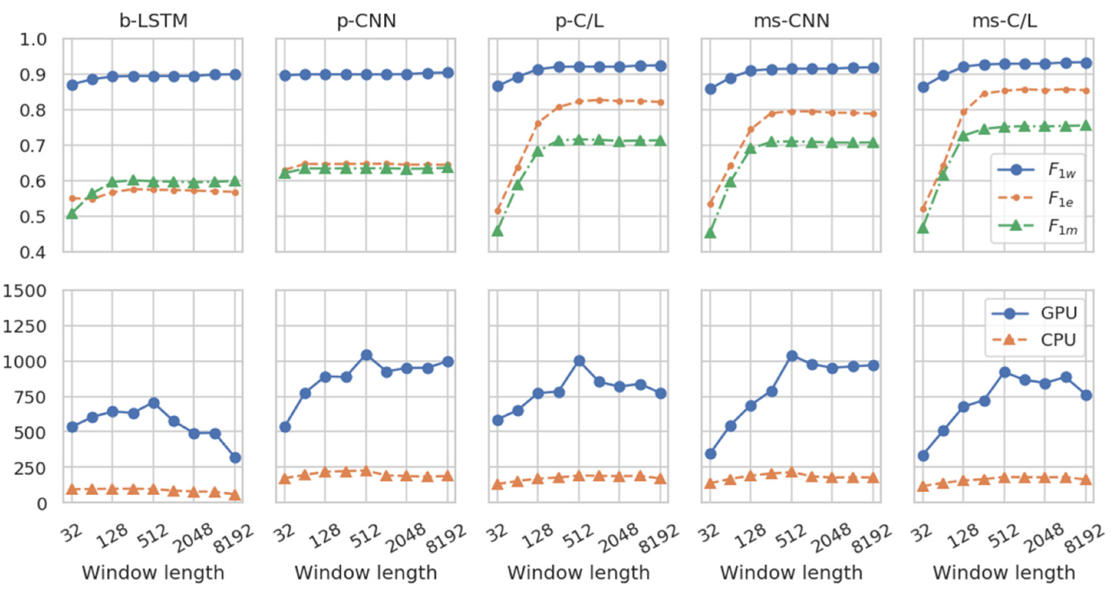
Figure 7.
Effects of inference window length. For all models, accuracy metrics (top panes) improve as inference window length increases, especially when models incorporate multi-scale or LSTM architectural features. For LSTM-containing models, the inference rate (bottom panes) falls off for long windows because their calculation across the time dimension cannot be fully parallelized. (n = 5 each).
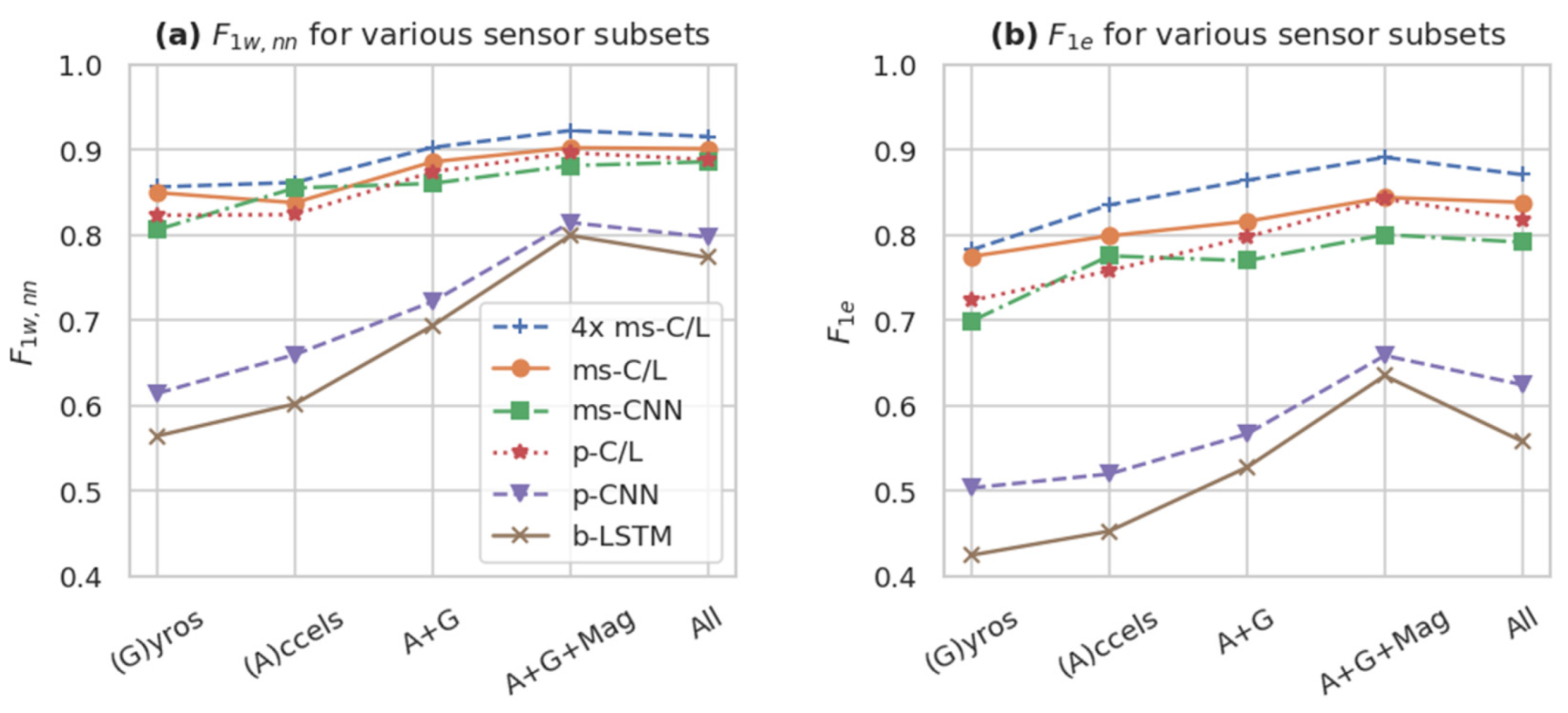
Figure 8.
Performance of different Opportunity sensor subsets (mean of n = 5 runs) according to (a) the sample-by-sample and (b) the event-based F1 . Using larger sensor subsets, including gyroscopes (G), accelerometers (A), and the magnetic (Mag) components of the inertial measurement units, as well as all 113 standard sensors channels (All), tended to improve performance metrics. The best models (e.g., 4× ms-C/L, ms-C/L, ms-CNN, and p-C/L) maintain relatively high performance even with fewer sensor channels.
Table 1.
Several FilterNet variants (and their abbreviated names). The variants range from simpler to more complex, using different combinations of components A-G. CNN: convolutional neural network; LSTM: long short-term memory.
Table 1.
Several FilterNet variants (and their abbreviated names). The variants range from simpler to more complex, using different combinations of components A-G. CNN: convolutional neural network; LSTM: long short-term memory.
| Variant | Components |
|---|
| A | B | C | D | E | F | G |
|---|
| Base LSTM (b-LSTM) 1 | - | - | - | - | - | ✓ | ✓ |
| Pooled CNN (p-CNN) | ✓ | ✓ | - | - | - | - | ✓ |
| Pooled CNN/LSTM (p-C/L) | ✓ | ✓ | - | - | - | ✓ | ✓ |
| Multi-Scale CNN (ms-CNN) | ✓ | ✓ | ✓ | ✓ | ✓ | - | ✓ |
| Multi-Scale CNN/LSTM (ms-C/L) | ✓ | ✓ | ✓ | ✓ | ✓ | ✓ | ✓ |
Table 2.
Configuration of the reference architectures used in this article. Each configuration represents one of the named FilterNet variants.
Table 2.
Configuration of the reference architectures used in this article. Each configuration represents one of the named FilterNet variants.
| Component | b-LSTM | p-CNN | p-C/L | ms-CNN | ms-C/L |
|---|
| A—Full-Res CNN | - | |
| B—Pooling Stack 1 | |
|
| C—Pooling Stack 2 | - |
|
| D—Resampling Step | - | 195 output channels 1 |
| E—Bottleneck Layer | - | |
| F—Recurrent Layers | | - | | - | |
| G—Output Module | |
Table 3.
Layer-by-layer configuration and description of the multi-scale CNN/LSTM (ms-C/L), the most complex reference architecture.
Table 3.
Layer-by-layer configuration and description of the multi-scale CNN/LSTM (ms-C/L), the most complex reference architecture.
| Component | Type | Win | Wout | | | Params1 | Output Stride Ratio2 | ROI3 |
|---|
| in | input | 113 4 | | | | | | 1 |
| A | | 113 4 | 100 | 1 | 5 | 56,700 4 | 1 | 5 |
| B | | 100 | 100 | 2 | 5 | 50,200 | 2 | 13 |
| B | | 100 | 100 | 2 | 5 | 50,200 | 4 | 29 |
| B | | 100 | 100 | 2 | 5 | 50,200 | 8 | 61 |
| C | | 100 | 50 | 2 | 5 | 25,100 | 16 | 125 |
| C | | 50 | 25 | 2 | 5 | 6300 | 32 | 253 |
| C | | 25 | 13 | 2 | 5 | 1651 | 64 | 509 |
| C | | 13 | 7 | 1 | 5 | 469 | 64 | 765 |
| D | resample | 195 | 195 | | | | | 765 |
| E | | 195 | 100 | 1 | 1 | 19,700 | 8 | 765 |
| F | | 100 | 100 | 1 | | 80,500 | 8 | all |
| G | | 100 | 18 | 1 | 1 | 1818 | 8 | all |
| out | output | | 18 | | | | | all |
Table 4.
Training parameters used in this study, along with an approximate recommended range for consideration in similar applications.
Table 4.
Training parameters used in this study, along with an approximate recommended range for consideration in similar applications.
| Parameter | Value | Recommended Range |
|---|
| Max epochs | 100 | 50–150 |
| Initial learning rate | 0.001 | 0.0005–0.005 |
| Samples per batch | 5,000 | 2,500–10,000 |
| Training window step | 16 | 8–64 |
| Optimizer | Adam | Adam, RMSProp |
| Weight decay | 0.0001 | 0–0.001 |
| Patience | 10 | 5–15 |
| Learning rate decay | 0.95 | 0.9–1.0 |
| Window length | 512 | 64–1024 |
Table 5.
Model and results summary for the Opportunity dataset, the five FilterNet reference architectures, as well as three modifications of the ms-C/L architecture. The 4-fold ms-C/L variant exhibited the highest accuracy, while smaller and simpler variants were generally faster but less accurate. The best results are in bold.
| | | Architecture | Classification Metrics | Efficiency |
|---|
| Model | n1 | Stride Ratio | Params (k) | | | | | kSamp/s | Trains/epoch |
|---|
| | FilterNet reference architectures |
| b-LSTM | 9 | 1 | 87 | 0.895 | 0.595 | 0.566 | 0.787 | 865 | 15 |
| p-CNN | 9 | 8 | 209 | 0.900 | 0.638 | 0.646 | 0.803 | 1340 | 2.0 |
| p-C/L | 9 | 8 | 299 | 0.922 | 0.717 | 0.822 | 0.883 | 1160 | 4.0 |
| ms-CNN | 9 | 8 | 262 | 0.919 | 0.718 | 0.792 | 0.891 | 1140 | 3.5 |
| ms-C/L | 9 | 8 | 342 | 0.928 | 0.743 | 0.842 | 0.903 | 1060 | 5.1 |
| | Other variants |
| 4-fold ms-C/L | 10 | 8 | 1371 | 0.933 | 0.755 | 0.872 | 0.918 | 303 | 5.1 × 4 |
| ½ scale ms-C/L | 9 | 8 | 100 | 0.921 | 0.699 | 0.815 | 0.880 | 1350 | 5.2 |
| 2x scale ms-C/L | 9 | 8 | 1250 | 0.927 | 0.736 | 0.841 | 0.901 | 682 | 7.0 |
| | Non-FilterNet models |
| DeepConvLSTM reimplementation | 20 | 12 | 3965 | -- | -- | -- | -- | 9 | 170 |
Table 6.
Model mean F1 score without nulls (
) for different sensor subsets (
n = 5 each). This table reproduces the multimodal fusion analysis of [
33]. The ms-C/L and 4-fold ms-C/L models improve markedly upon reported DeepConvLSTM performance, especially with smaller sensor subsets. The best results are in bold.
| | Gyros | Accels | Accels+ Gyros | Accels+ Gyros + Magnetic | Opportunity Sensors Set |
|---|
| # of sensor channels | 15 | 15 | 30 | 45 | 113 |
| DeepConvLSTM [33] | 0.611 | 0.689 | 0.745 | 0.839 | 0.864 |
| p-CNN | 0.615 | 0.660 | 0.722 | 0.815 | 0.798 |
| ms-C/L | 0.850 | 0.838 | 0.886 | 0.903 | 0.901 |
| 4-fold ms-C/L | 0.857 | 0.862 | 0.903 | 0.923 | 0.916 |
Table 7.
Performance comparison alongside published models on the Opportunity dataset. FilterNet models perform set records in each metric. The best results are in bold.
Table 7.
Performance comparison alongside published models on the Opportunity dataset. FilterNet models perform set records in each metric. The best results are in bold.
| Method/Model | | | | | n |
|---|
| DeepConvLSTM | [33] | 0.672 | 0.915 | 0.866 | ? |
| LSTM-S | [36] | 0.698 | 0.912 | | best of 128 |
| 0.619 | | | median of 128 |
| b-LSTM-S | [36] | 0.745 | 0.927 | | best of 128 |
| 0.540 | | | median of 128 |
| LSTM Ensembles | [39] | 0.726 | | | mean of 30 |
| Res-Bidir-LSTM | [51] | | 0.905 | | ? |
| Asymmetric Residual Network | [52] | | 0.903 | | ? |
| DeepConvLSTM + Attention | [53] | 0.707 | | | mean |
| FilterNet ms-CNN | | 0.718 | 0.919 | 0.891 | mean of 9 |
| FilterNet ms-C/L | | 0.743 | 0.928 | 0.903 | mean of 9 |
| FilterNet 4-fold ms-C/L | | 0.755 | 0.933 | 0.918 | mean of 10 |


