Design, Implementation and Data Analysis of an Embedded System for Measuring Environmental Quantities †


Abstract
1. Introduction
Related Work
2. Materials and Methods
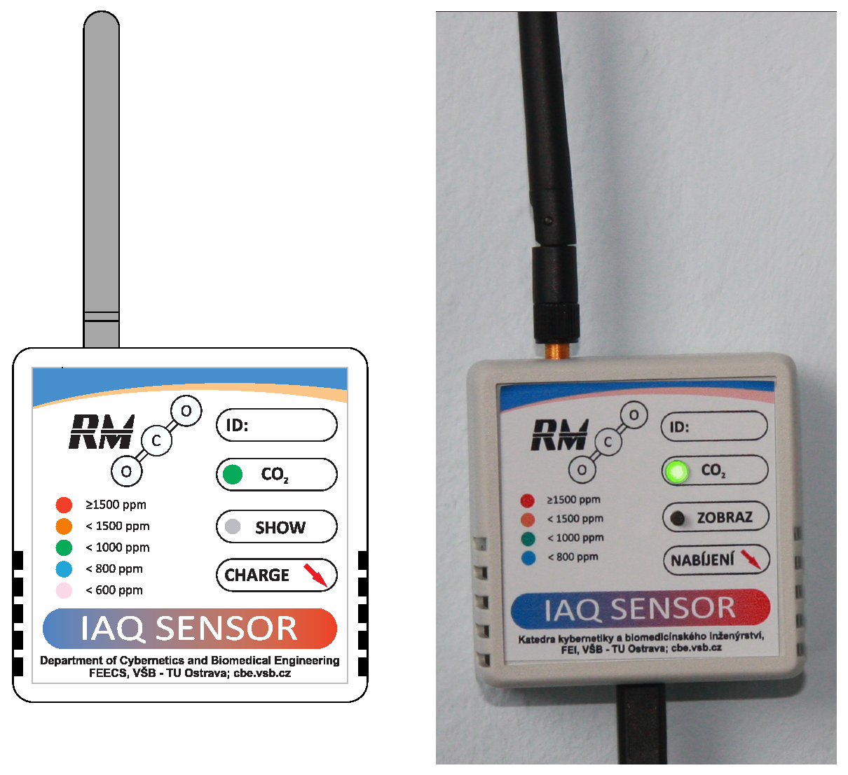
2.1. Carbon Dioxide Measurement Device
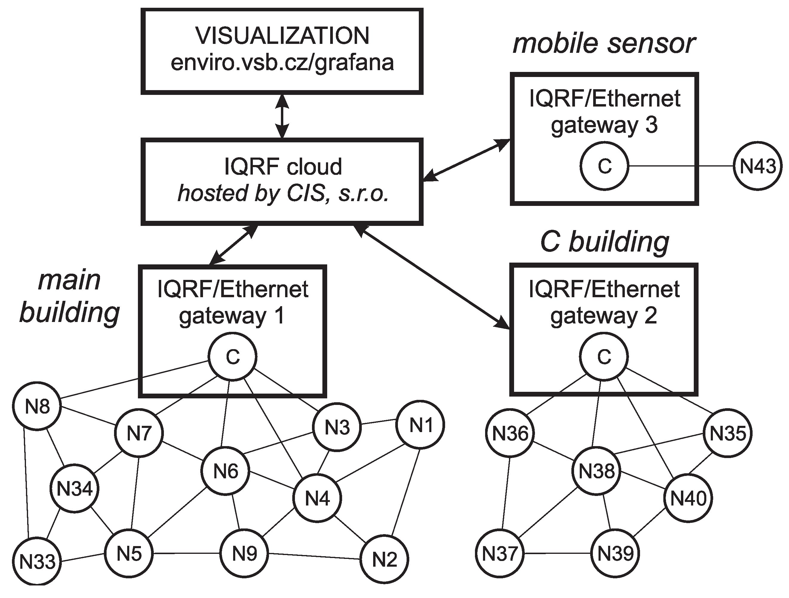
2.2. Measurement Network
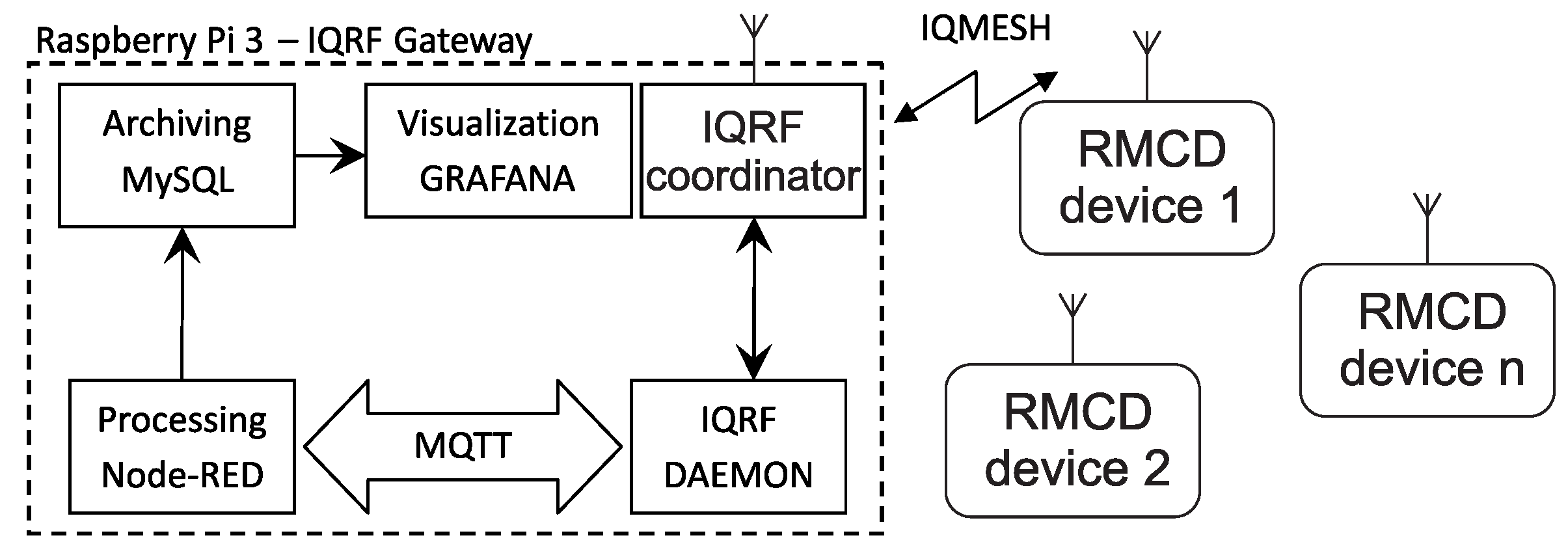
- RMCD device—transmits measured CO2 concentration, temperature and relative humidity of ambient air, and atmospheric pressure data upon request.
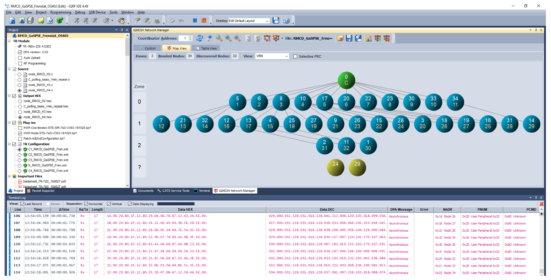
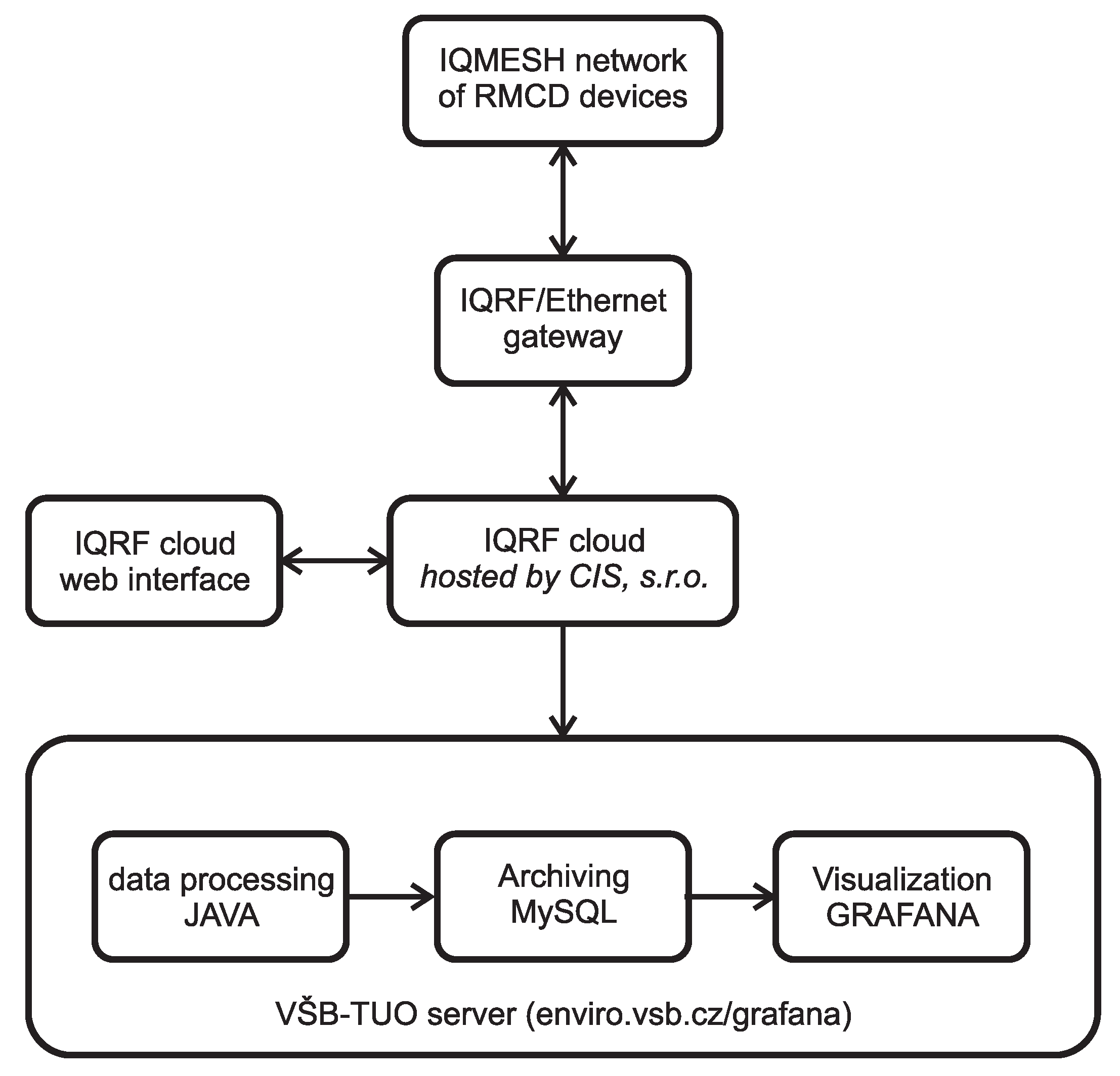
- IQRF®/Ethernet gateway contains a network coordinator, microcontroller and Ethernet interface for internet connectivity. This device works in two modes either as a datalogger or a gateway. In datalogger mode, all data received from an IQRF® network is sent to the cloud, or vice versa, data are transmitted from the cloud to the IQRF® network. Gateway mode allows messages to be transmitted from the IQRF® network to the IQRF® IDE development environment. This mode enables the remote setting of IQRF® network parameters, such as adding or removing network nodes. The gateway also works with the UDP channel, providing communication with the IQRF® IDE development environment as well as an MQTT broker with the Node-RED tool.
- IQRF® Cloud—a commercial service that collects IQRF® data from IQRF®/GSM or IQRF®/Ethernet gateway. This cloud enables bi-directional data transfer, i.e., from the gateway to the cloud and the cloud to the gateway. The gateway must be set in datalogger mode.
- Visualization—measured data are visualized using Grafana software. This SW is installed on the VŠB-TUO server. The basis of each visualization tool is a data source. In our case studies, we have used the MySQL database, which was also installed on the university server enviro.vsb.cz [38] (login: sensors, password: sensors). For each IQRF®/Ethernet gateway, a table is created in the database where processed data from the IQRF® cloud are stored. Grafana is also accessible from outside the university network, therefore dashboards can be viewed from anywhere as long as access to the Internet is available.
3. Analysis of Carbon Dioxide Measurements
3.1. Case Study—Department of Cybernetics and Biomedical Engineering, VŠB-Technical University of Ostrava
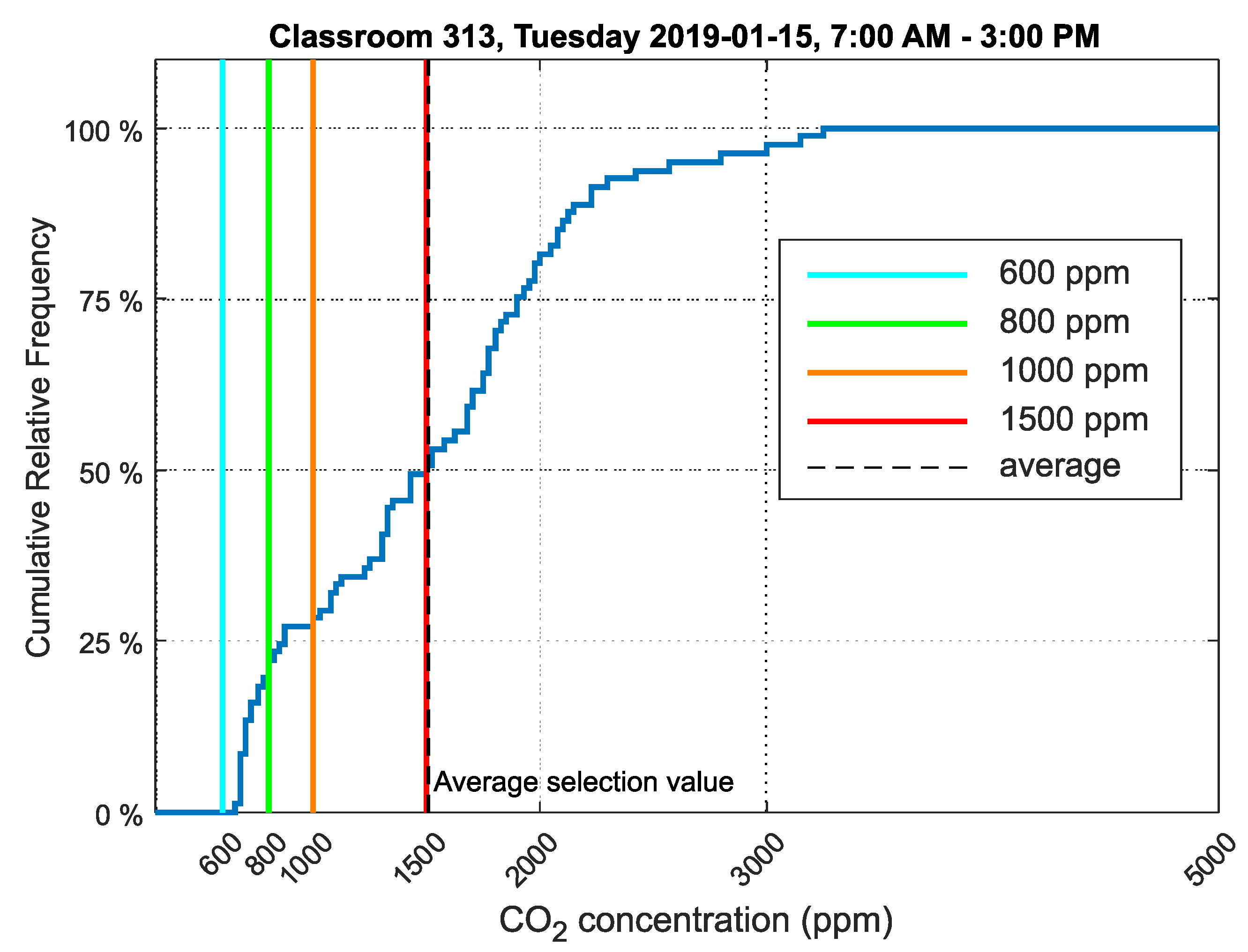
3.2. Case Study–Grammar School and Secondary School of Electrical Engineering and Computer Science, Frenštát pod Radhoštěm
4. Results
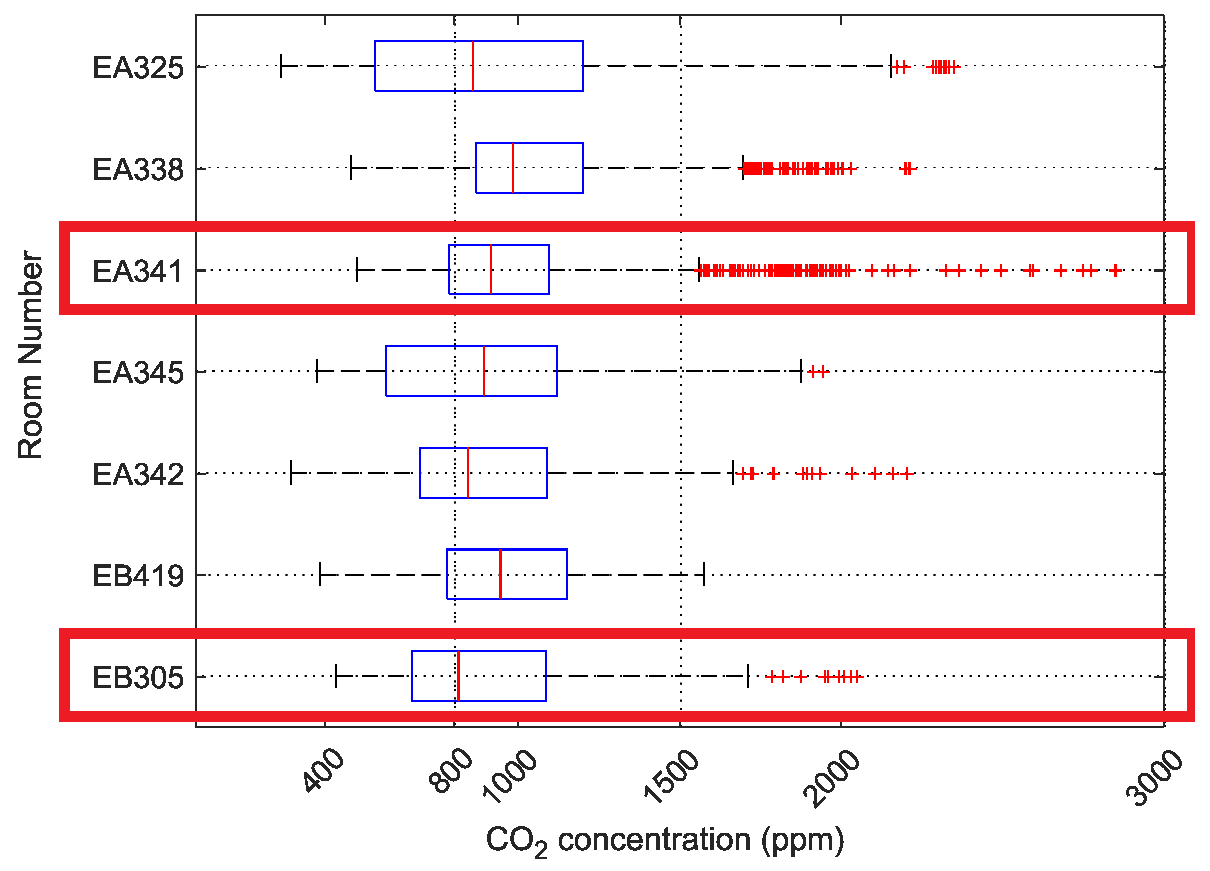
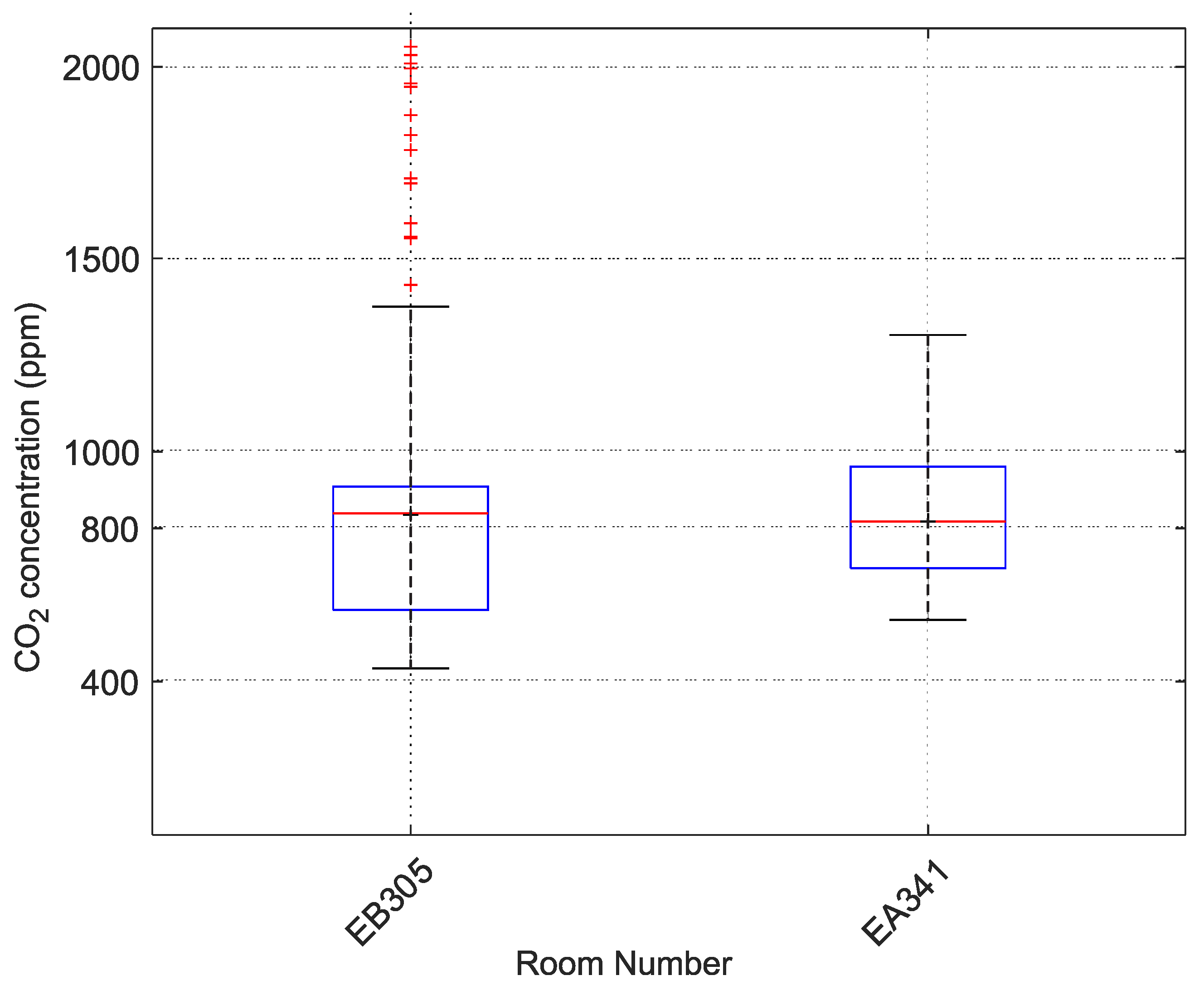
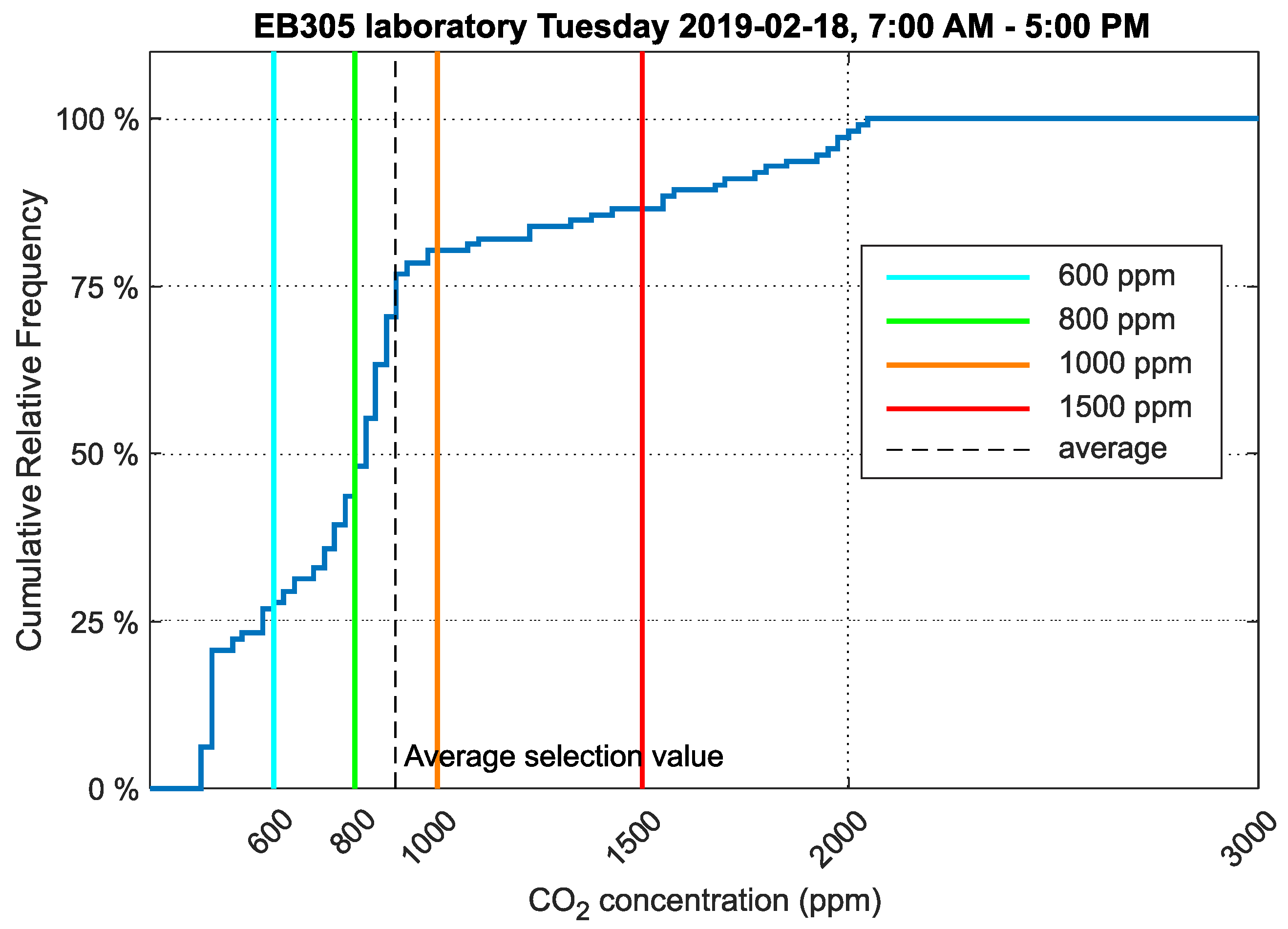
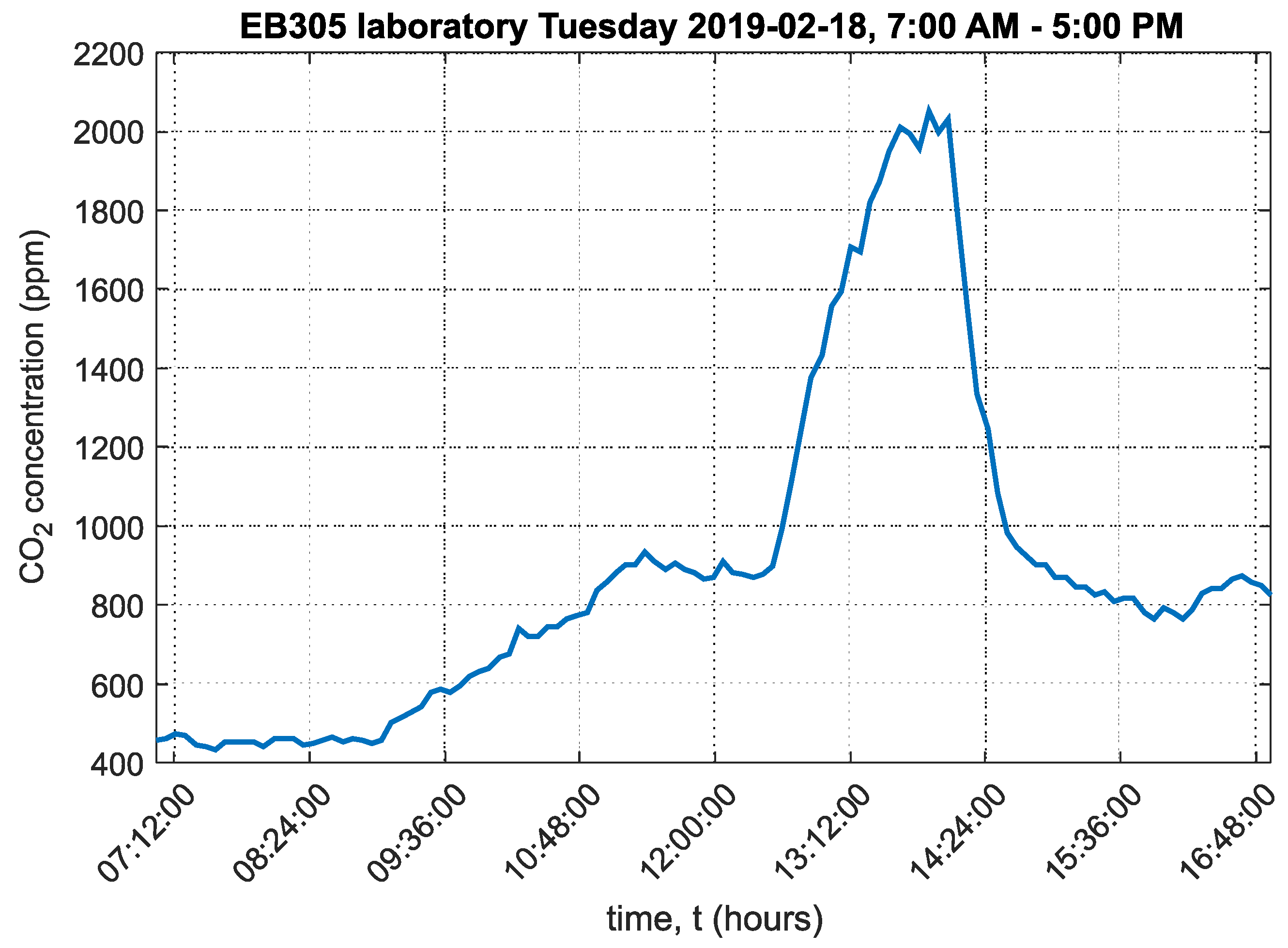
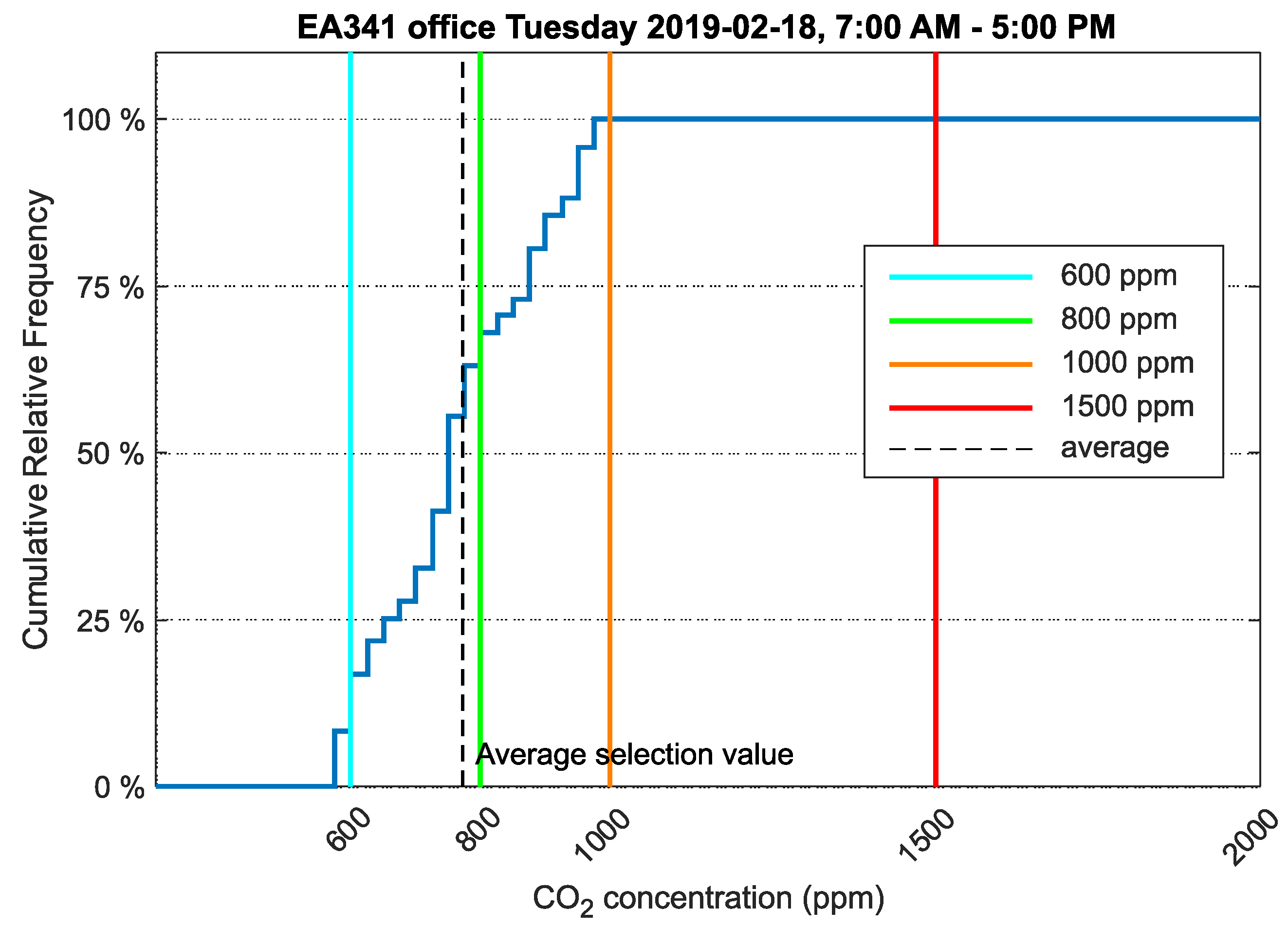
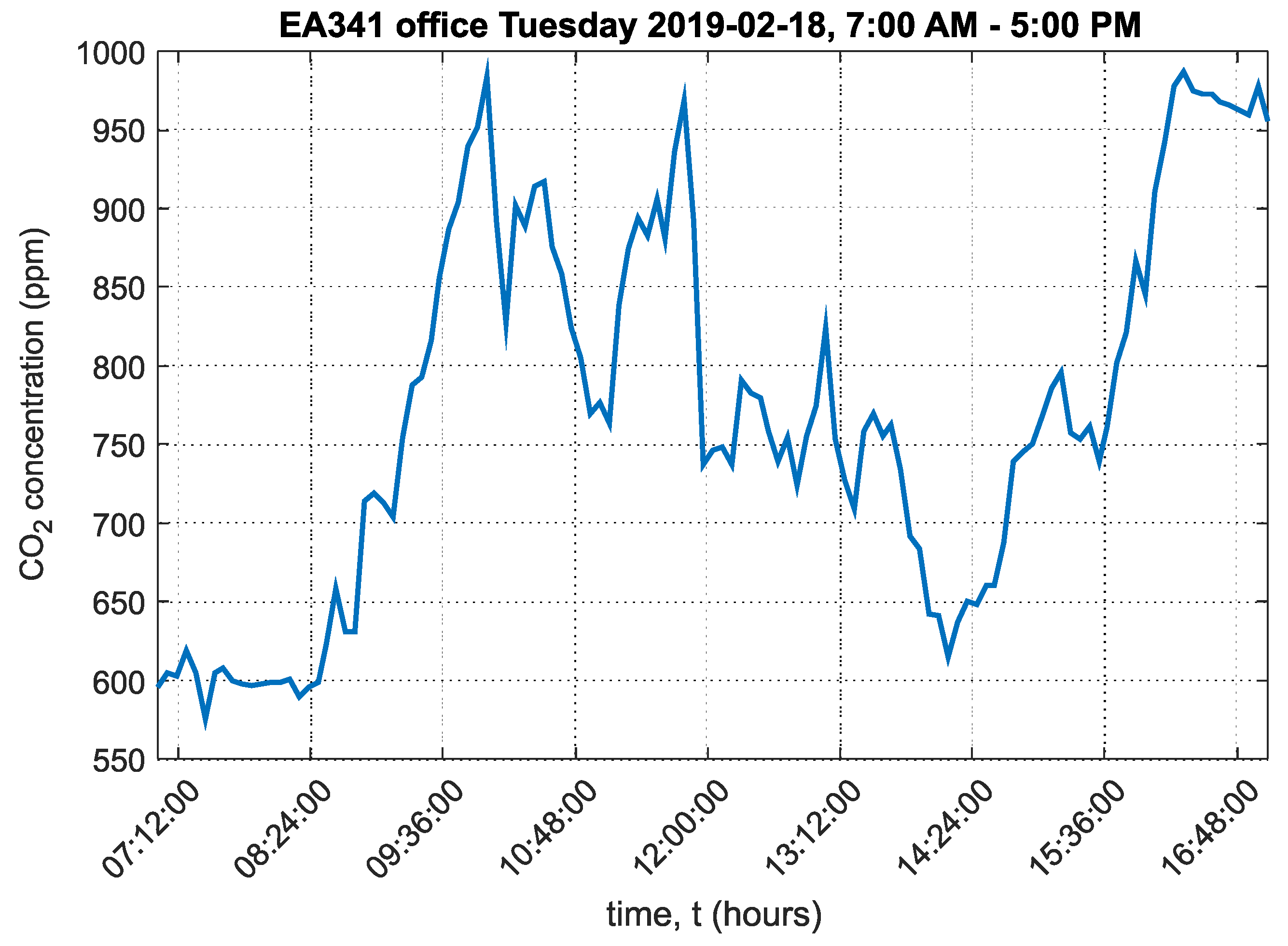
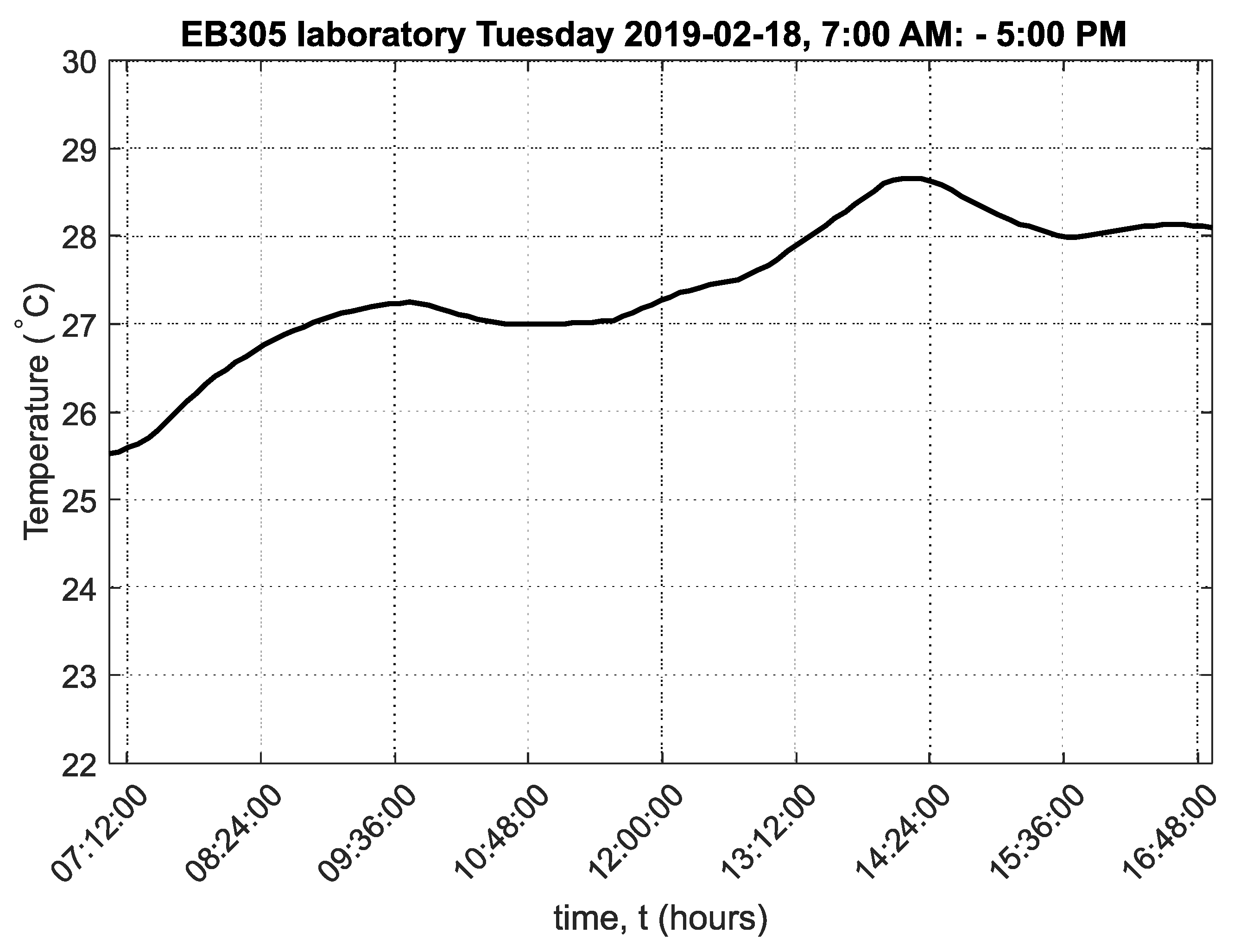
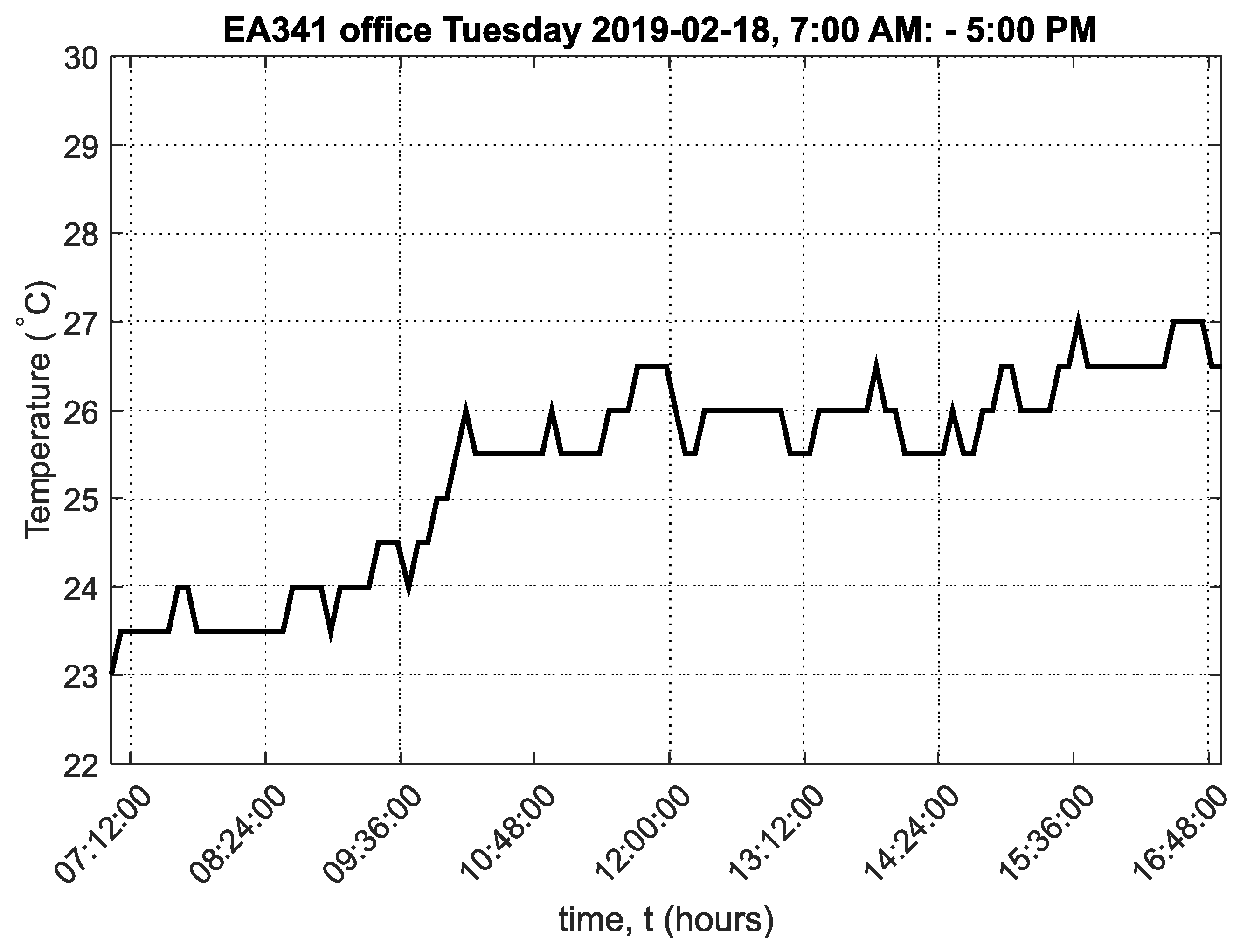
4.1. Department of Cybernetics and Biomedical Engineering, VŠB-Technical University of Ostrava
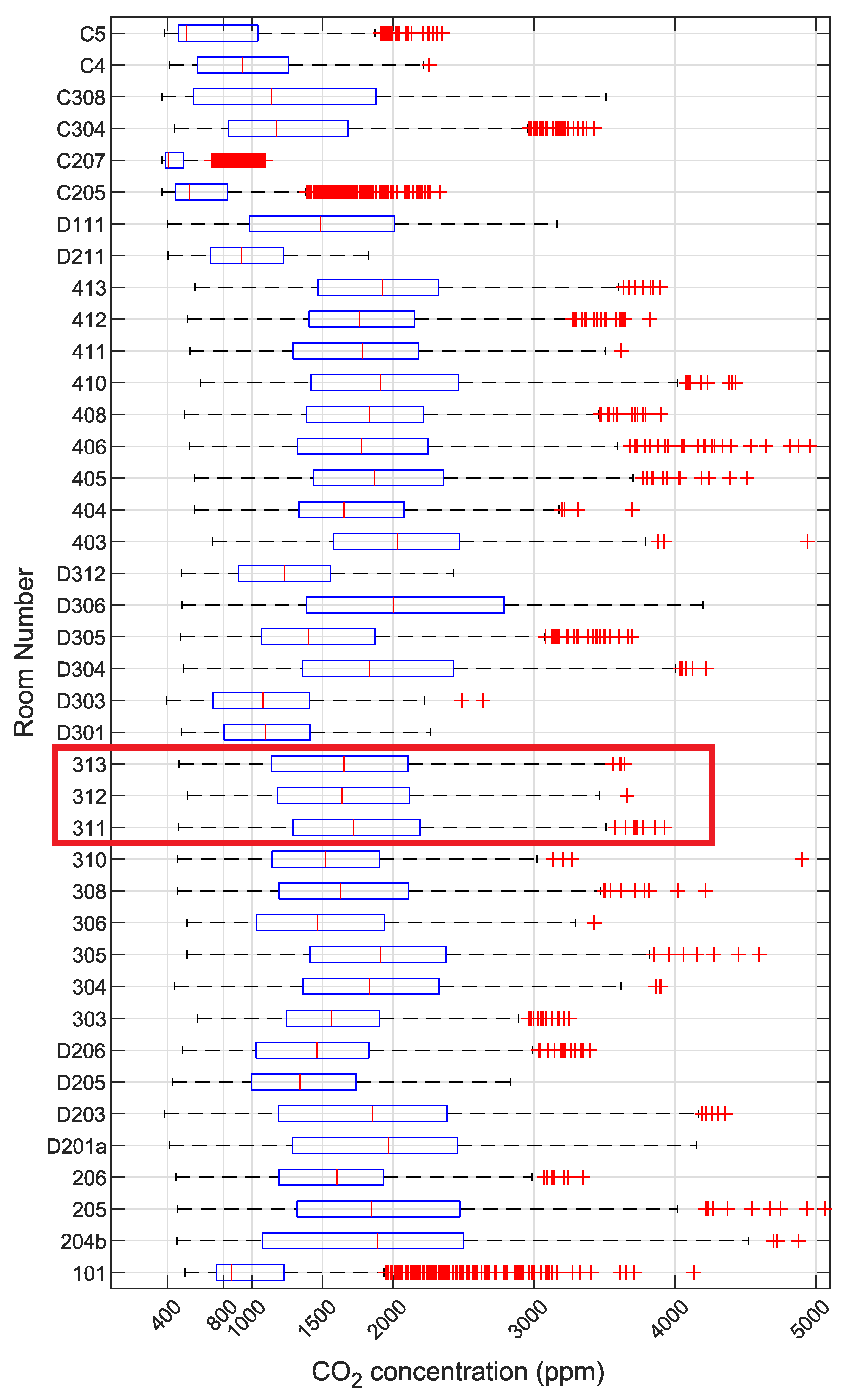
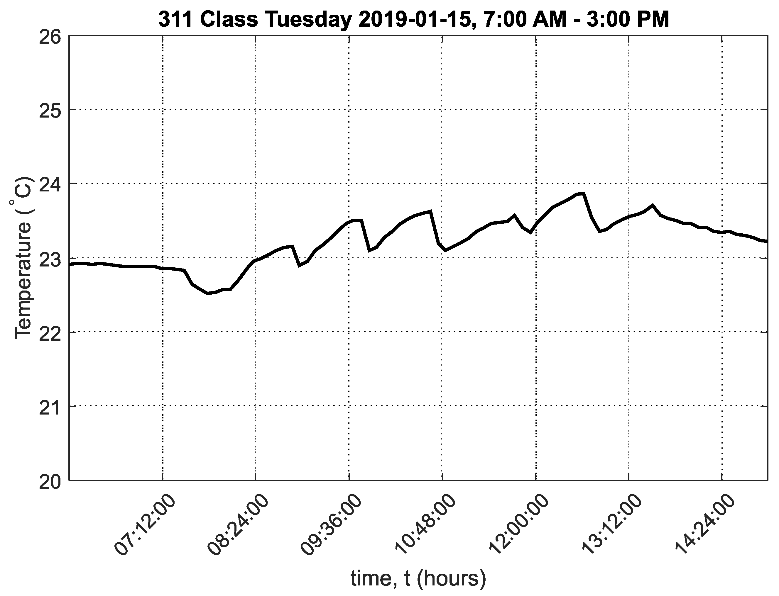
4.2. Grammar School and Secondary School of Electrical Engineering and Computer Science, Frenštát pod Radhoštěm
5. Conclusions
Author Contributions
Funding
Acknowledgments
Conflicts of Interest
Abbreviations
| BLE | Bluetooth Low Energy |
| CO2 | Carbon Dioxide |
| DPA | Direct Peripheral Access - byte-oriented protocol used to control IQMESH network services |
| EA341 | Name of the office at VŠB-TUO |
| EB305 | Name of the laboratory at VŠB-TUO |
| IQMESH | A topology type in an IQRF® wireless network |
| IQRF® | Trademark name of the wireless communication technology for the nodes and coordinator in the MESH topology network |
| JSON | JavaScript Object Notation—An open-standard file format or data interchange format that uses human-readable text to transmit data objects consisting of attribute-value pairs and array data types (or any other serializable value) |
| KNX | An open standard (see EN 50090, ISO/IEC 14543) for commercial and domestic building automation |
| LoRa | Long Range—A low-power wide-area network (LPWAN) technology working in license free sub-gigahertz band |
| MQTT | Message Queuing Telemetry Transport—machine-to-machine (M2M)/“Internet of Things” connectivity protocol |
| OTA | Over The Air—firmware changes over the wireless network |
| REST-API | Representational state transfer—Application Interface |
| RMCD | Room Measurement of Carbon Dioxide—A device for measuring CO2 concentration |
| MySQL | An open-source relational database management system |
| VŠB-TUO | Vysoká škola báňská—Tecnická univerzita Ostrava—name of the university |
Appendix A. Graphs of Other Measured Quantities
Appendix A.1. Department of Cybernetics and Biomedical Engineering, VŠB-Technical University of Ostrava


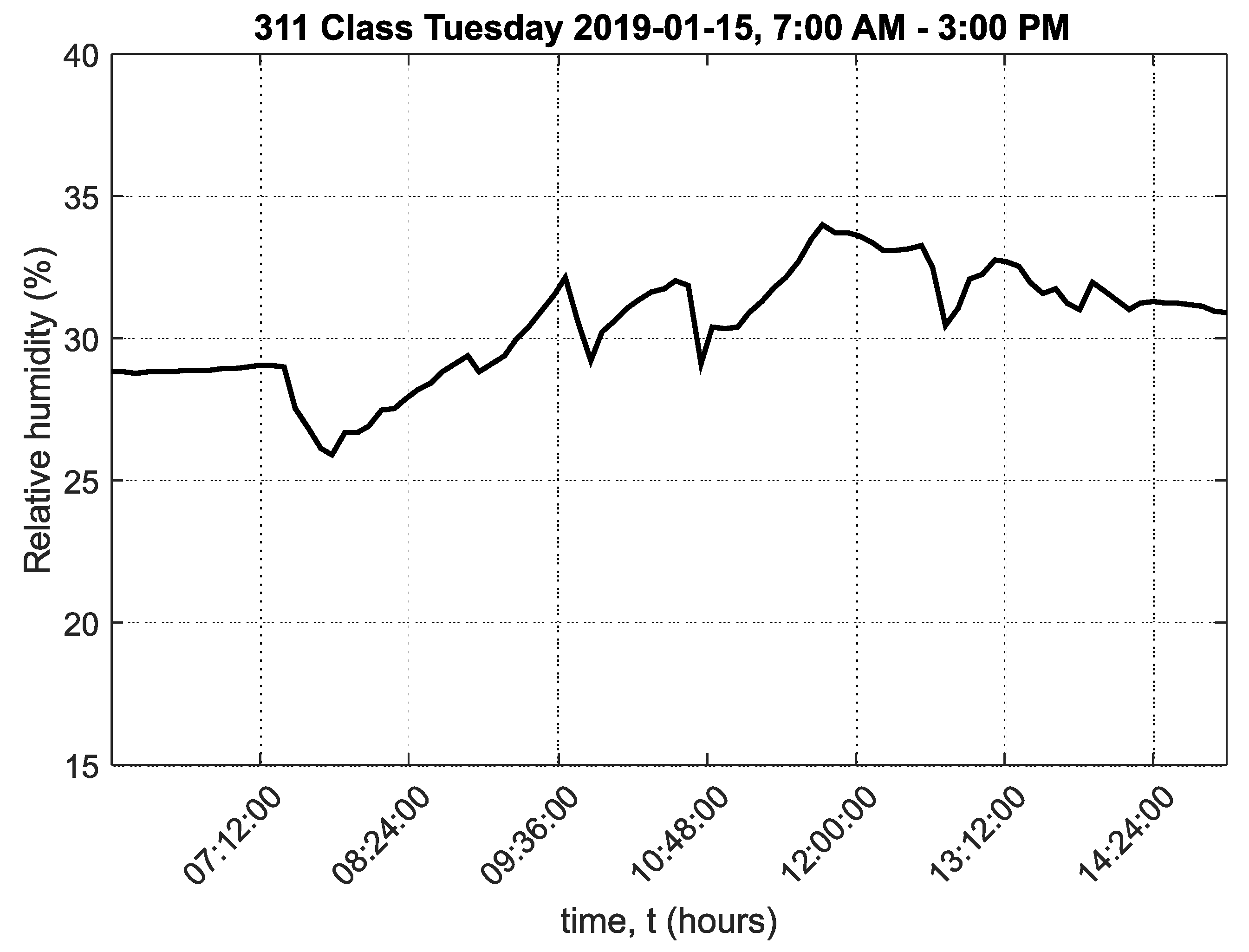
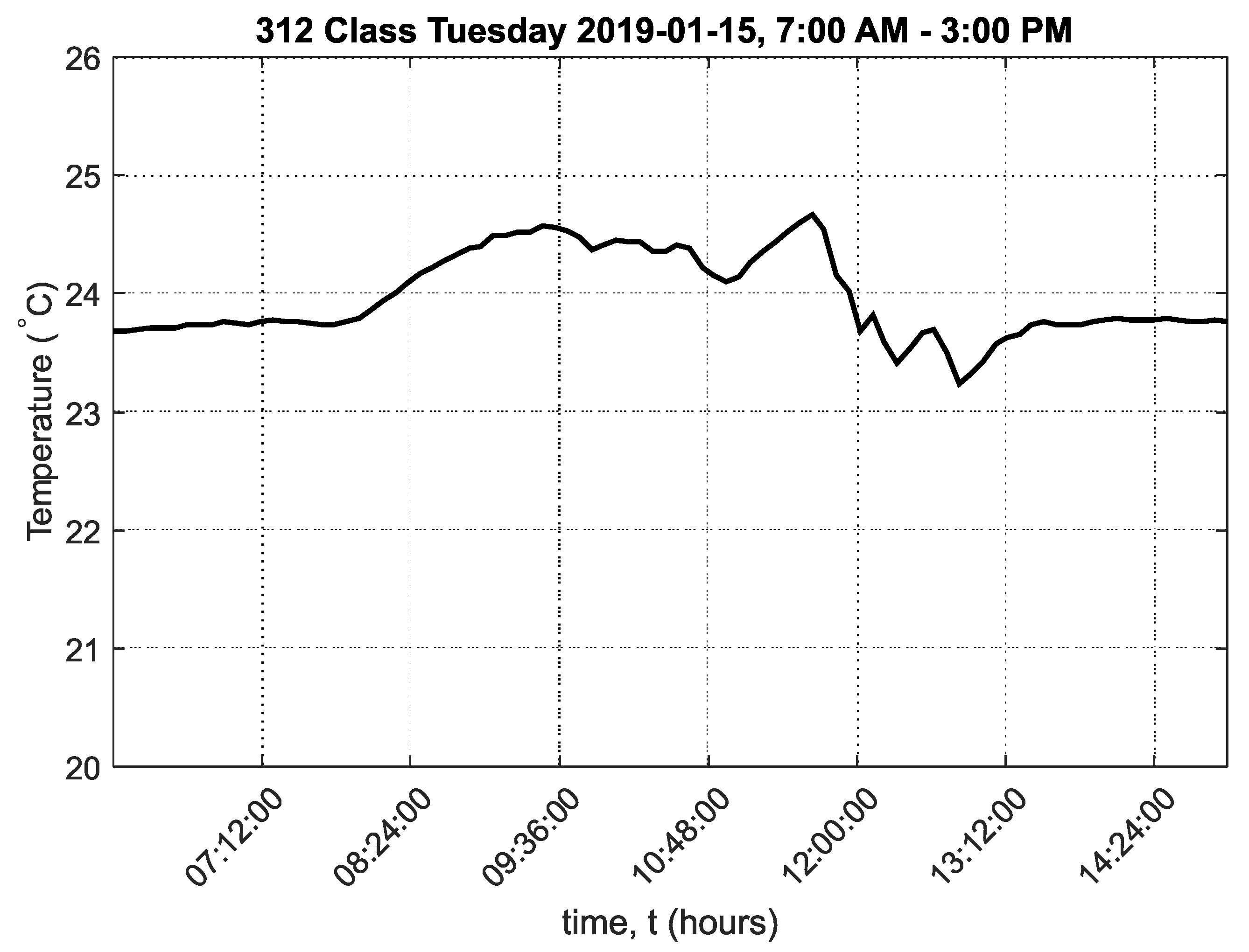
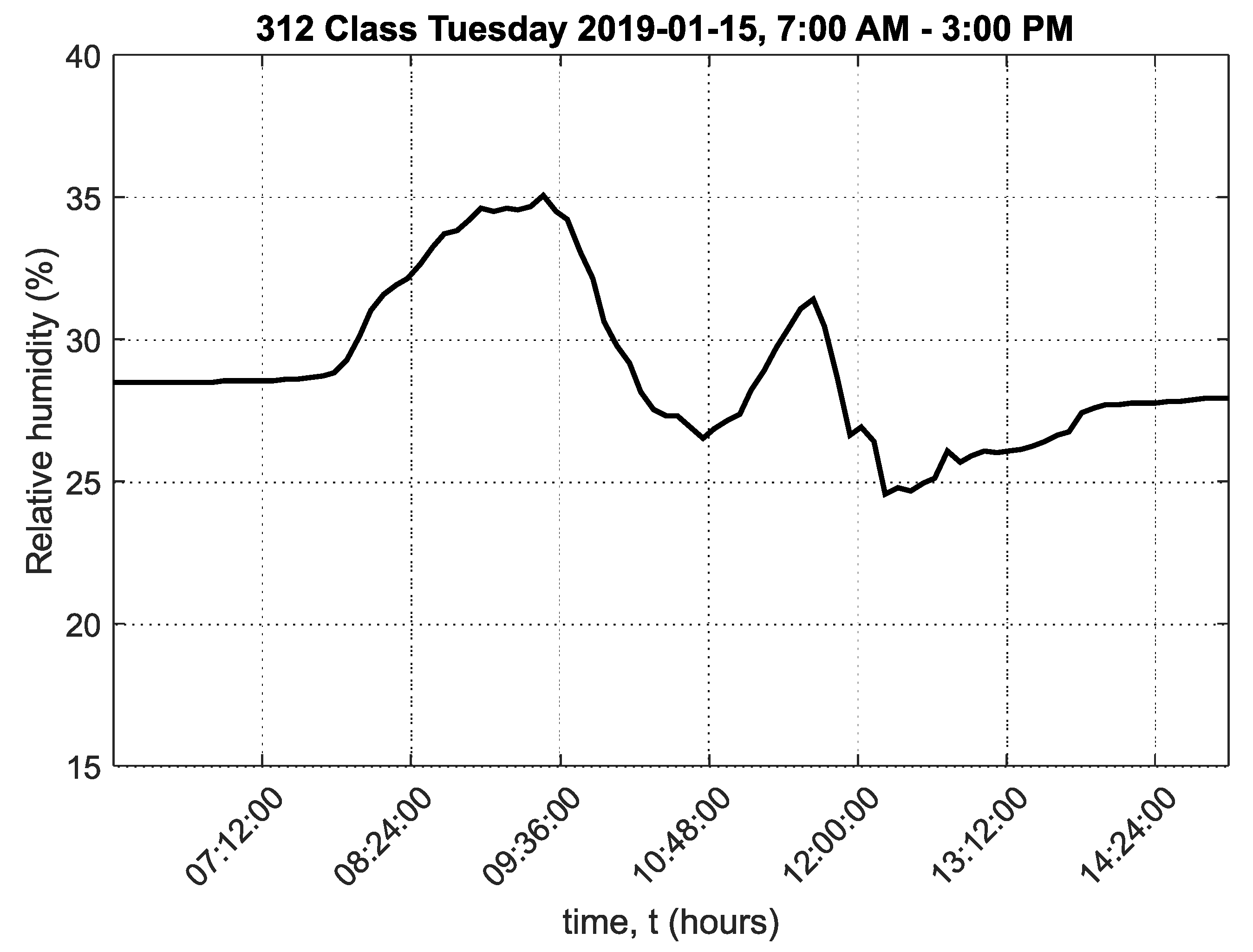
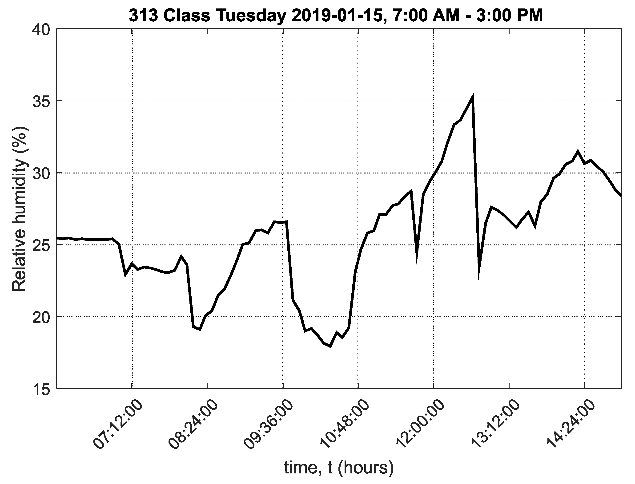
Appendix A.2. Grammar School and Secondary School of Electrical Engineering and Computer Science, Frenštát pod Radhoštěm


References
- Gecova, K.; Vala, D.; Slanina, Z.; Walendziuk, W. Air Condition Sensor on KNX Network. In Proceedings of SPIE—The International Society for Optical Engineering; Linczuk, M., Romaniuk, R., Eds.; SPIE: Bellingham, WA, USA, 2017; Volume 10445. [Google Scholar] [CrossRef]
- Velicka, J.; Pies, M.; Hajovsky, R. Monitoring of Environmental Variables in Rooms of the Department of Cybernetics and Biomedical Engineering. In 2018 IEEE 20th International Conference on e-Health Networking, Applications and Services (Healthcom); Institute of Electrical and Electronics Engineers Inc.: Piscataway, NJ, USA, 2018. [Google Scholar] [CrossRef]
- Velicka, J.; Pies, M.; Hajovsky, R. Wireless Measurement of Carbon Dioxide by use of IQRF Technology. IFAC-PapersOnLine 2018, 51, 78–83. [Google Scholar] [CrossRef]
- Velicka, J. Measuring and Visualization System for Measuring Environmental Quantities using IQRF. Master’s Thesis, VSB-Technical University of Ostrava, Department of Cybernetics and Biomedical Engineering, Ostrava, Czech Republic, 2018. [Google Scholar]
- Eusebio, L.; Derudi, M.; Capelli, L.; Nano, G.; Sironi, S. Assessment of the Indoor Odour Impact in a Naturally Ventilated Room. Sensors 2017, 17, 778. [Google Scholar] [CrossRef] [PubMed]
- Salamone, F.; Belussi, L.; Danza, L.; Galanos, T.; Ghellere, M.; Meroni, I. Design and Development of a Nearable Wireless System to Control Indoor Air Quality and Indoor Lighting Quality. Sensors 2017, 17, 1021. [Google Scholar] [CrossRef] [PubMed]
- IQRF Tech s.r.o. IQRF—Technology for Wireless. Available online: https://www.iqrf.org/ (accessed on 22 January 2020).
- Calvo, I.; Gil-García, J.; Recio, I.; López, A.; Quesada, J. Building IoT Applications with Raspberry Pi and Low Power IQRF Communication Modules. Electronics 2016, 5, 54. [Google Scholar] [CrossRef]
- Pies, M.; Hajovsky, R.; Velicka, J. Design and Implementation of the Embedded System for Environmental Variables Measurement. In Proceedings of the 5th International Conference on Sensors Engineering and Electronics Instrumentation Advances (SEIA’ 2019), Tenerife, Spain, 25–27 September 2019. [Google Scholar]
- Protronix. New NL-ECO-CO2 Sensor. Available online: https://www.careforair.eu/en/produkty/co2-sensors/new-nl-eco-co2-2/ (accessed on 22 March 2020).
- Protronix. NLII-CO2+RH-R-5 Sensor. Available online: https://www.careforair.eu/en/produkty/combined-sensors/co2-and-relative-humidity-sensors/nlii-co2rh-r-5-sensor/ (accessed on 15 April 2020).
- Extech. SD800: CO2, Humidity and Temperature Datalogger. Available online: http://www.extech.com/products/SD800 (accessed on 20 March 2020).
- Marchetti, N.; Cavazzini, A.; Pasti, L.; Catani, M.; Malagu, C.; Guidi, V. A campus sustainability initiative: Indoor air quality monitoring in classrooms. In Proceedings of the 2015 18th AISEM Annual Conference (AISEM 2015), Trento, Italy, 3–5 February 2015. [Google Scholar] [CrossRef]
- Spachos, P.; Hatzinakos, D. Real-Time Indoor Carbon Dioxide Monitoring Through Cognitive Wireless Sensor Networks. IEEE Sens. J. 2016, 16, 506–514. [Google Scholar] [CrossRef]
- Guangzhou MCOHome Technology Co., Ltd. CO2 Monitor MH9 Series. Available online: http://www.mcohome.com/show_list.php?id=44&sid=51 (accessed on 20 March 2020).
- ALTERNETIVO. LS-111 CO2 + Temp/Humidity SensorLoRaWAN EU 868 MHz. Available online: https://www.alternetivo.cz/ls-111-co2-teplota-vlhkost-senzor-lorawan_d60166.html (accessed on 22 March 2020).
- Mekki, K.; Bajic, E.; Chaxel, F.; Meyer, F. Overview of Cellular LPWAN Technologies for IoT Deployment: Sigfox, LoRaWAN, and NB-IoT. In Proceedings of the 2018 IEEE International Conference on Pervasive Computing and Communications Workshops (PerCom Workshops 2018), Athens, Greece, 19–23 March 2018; pp. 197–202. [Google Scholar] [CrossRef]
- Sigfox. Buy Sigfox Connectivity for Your IoT Devices. Available online: https://buy.sigfox.com/buy/offers/FR (accessed on 14 April 2020).
- GlobalSat WorldCom Corporation. GlobalSat LS-111. Available online: https://www.globalsat.com.tw/en/product-225265/CO2-and-Temperature-Humidity-Detector-with-LoRaWAN%E2%84%A2-Certified-Module-LS-111P.html (accessed on 23 March 2020).
- LORATECH.CZ. Gateway to the World of Internet of Things. Available online: http://chytra-obec.cz/en/ (accessed on 14 April 2020).
- Firdaus, R.; Murti, M.; Alinursafa, I. Air quality monitoring system based internet of things (IoT) using LPWAN LoRa. In Proceedings of the 2019 IEEE International Conference on Internet of Things and Intelligence System (IoTaIS 2019), Bali, Indonesia, 5–7 November 2019; pp. 195–200. [Google Scholar] [CrossRef]
- Cheong, P.; Bergs, J.; Hawinkel, C.; Famaey, J. Comparison of LoRaWAN classes and their power consumption. In Proceedings of the 2017 IEEE Symposium on Communications and Vehicular Technology (SCVT 2017), Leuven, Belgium, 14 November 2017; pp. 1–6. [Google Scholar] [CrossRef]
- Andrade, R.; Yoo, S. A comprehensive study of the use of LoRa in the development of smart cities. Appl. Sci. 2019, 9, 4753. [Google Scholar] [CrossRef]
- Sulc, V. Microelectronic Wireless Networks for Telemetry and Buildings Automation. Ph.D. Thesis, Brno University of Technology, Faculty od Electrical Engineering and Communication, Department of Microelectronics, Brno, Czech Republic, 2015. [Google Scholar]
- IQRF Tech s.r.o. IQRF OS Operating System Version 4.03D for TR-7xD - User’s Guide. Available online: https://static.iqrf.org/User_Guide_IQRF-OS-403D_TR-7xD_191209.pdf (accessed on 24 March 2020).
- IQRF Tech s.r.o. IQRF DPA Framework—Technical Guide; Version v4.13; IQRF OS v4.03D. Available online: https://static.iqrf.org/Tech_Guide_DPA-Framework-413_200227.pdf (accessed on 24 March 2020).
- Figaro Japan. CDM7160 Non Dispersive Infrared (NDIR) CO2 Sensor. Available online: https://www.figaro.co.jp/en/product/feature/cdm7160.html (accessed on 14 January 2020).
- Hajovsky, R.; Pies, M. Use of IQRF Technology for Large Monitoring Systems. IFAC-PapersOnLine 2015, 28, 486–491. [Google Scholar] [CrossRef]
- Ursutiu, D.; Neagu, A.; Samoilă, C.; Jinga, V. MODULARITY applied to SMART HOME: From research to education. Lect. Notes Netw. Syst. 2018, 22, 56–67. [Google Scholar] [CrossRef]
- Hartová, V.; Hart, J. Improvement of monitoring of cattle in outdoor enclosure using IQRF technology. Agron. Res. 2018, 16, 410–415. [Google Scholar] [CrossRef]
- Fujdiak, R.; Mlynek, P.; Malina, L.; Orgon, M.; Slacik, J.; Blazek, P.; Misurec, J. Development of IQRF technology: Analysis, simulations and experimental measurements. Elektron. Elektrotech. 2019, 25, 72–79. [Google Scholar] [CrossRef]
- Krupka, L.; Vojtech, L.; Neruda, M. The Issue of LPWAN Technology Coexistence in IoT Environment. In Proceedings of the 2016 17th International Conference on Mechatronics-Mechatronika (ME); Stefek, A., Maga, D., Brezina, T., Eds.; Institute of Electrical and Electronics Engineers Inc.: Piscataway, NJ, USA, 2017. [Google Scholar]
- Seflova, P.; Sulc, V.; Pos, J.; Spinar, R. IQRF wireless technology utilizing IQMESH protocol. In Proceedings of the 2012 35th International Conference on Telecommunications and Signal Processing (TSP 2012), Prague, Czech Republic, 3–4 July 2012; pp. 101–104. [Google Scholar] [CrossRef]
- IQRF Tech s.r.o. IQMESH Animations. Available online: https://www.iqrf.org/technology/iqmesh (accessed on 21 March 2020).
- Pies, M.; Hajovsky, R. Monitoring Environmental Variables through Intelligent Lamps. In Lecture Notes in Electrical Engineering; Joukov, N., Kim, K.J., Eds.; Springe: Singapore, 2018; Volume 425, pp. 148–156. [Google Scholar] [CrossRef]
- Slanina, Z.; Hajovsky, R.; Cepelak, M.; Walendziuk, W. Strain Gauge Sensor for the Internet of Things. In Proceedings of the SPIE—The International Society for Optical Engineering; SPIE: Bellingham, WA, USA, 2019; Volume 11176. [Google Scholar] [CrossRef]
- Hajovsky, R.; Pies, M.; Velicka, J. Monitoring the Condition of the Protective Fence above the Railway Track. IFAC-PapersOnLine 2019, 52, 145–150. [Google Scholar] [CrossRef]
- VSB-TU Ostrava. Dashboard for Monitoring the Environmental Quantities. Available online: http://enviro.vsb.cz/grafana/ (accessed on 29 February 2020).


| Min. Value | Rec. Value | Max. Value | |
|---|---|---|---|
| CO2 concentration (ppm) | - | 800–1000 | 1500 |
| Temperature (°C) | 20 (except. 18) | 20–24 | 28 (except. 30) |
| Relative humidity (%) | 30 | 30–64 | 70 |
| Lesson | 1 | 2 | 3 | 4 |
|---|---|---|---|---|
| Time | 8:00 AM–8:45 AM | 8:55 AM–9:40 AM | 9:50 AM–10:35 AM | 10:55 AM–11:40 AM |
| 311 | 6th class | 6th class | 2nd class | 6th class |
| 312 | 7th and 3rd class | 7th and 3rd class | 7th class | 7th class |
| 313 | 2nd class | 2nd class | free | 2nd |
| Lesson | 5 | 6 | 7 | |
| Time | 11:50 AM–12:35 PM | 12:45 PM–13:30 PM | 13:35 PM–14:20 PM | |
| 311 | 6th class | 4th class | free | |
| 312 | 2nd class | 5th class | free | |
| 313 | 2nd class | 4th class | 8th class |
| Room Number | Mean (ppm) | Min (ppm) | Max (ppm) | Standard Deviation (ppm) |
|---|---|---|---|---|
| EB305 laboratory | 916 | 434 | 2051 | 484 |
| EA341 office | 792 | 561 | 1088 | 150 |
| Room Number | Variation (ppm2) | Median (ppm) | under 1500 ppm (%) | |
| EB305 laboratory | 234,139 | 856 | 84 | |
| EA341 office | 22,515 | 787 | 100 |
| Room Number | Mean (ppm) | Min (ppm) | Max (ppm) | Standard Deviation (ppm) |
|---|---|---|---|---|
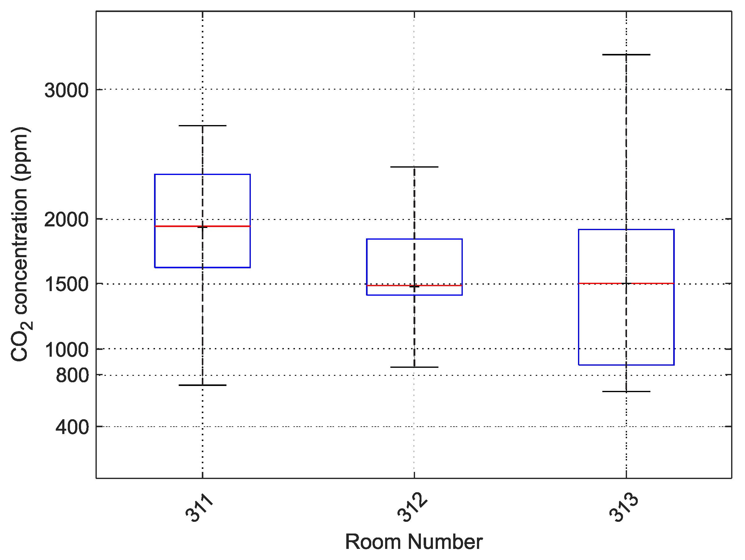
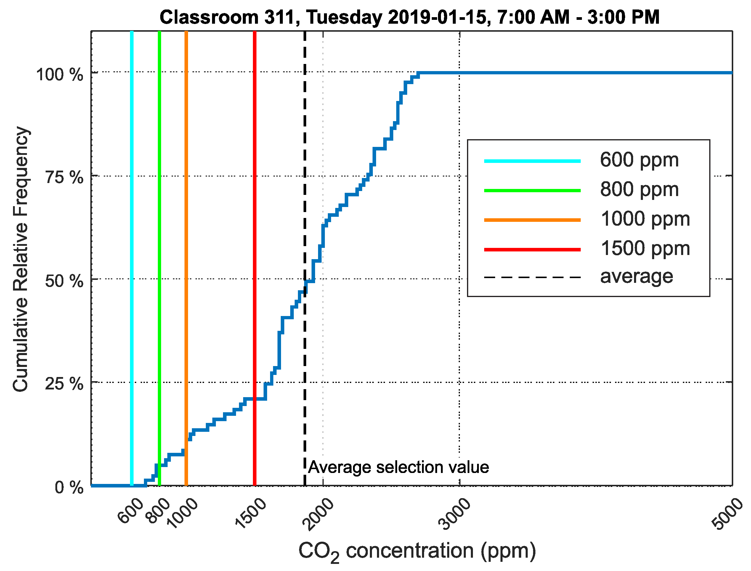
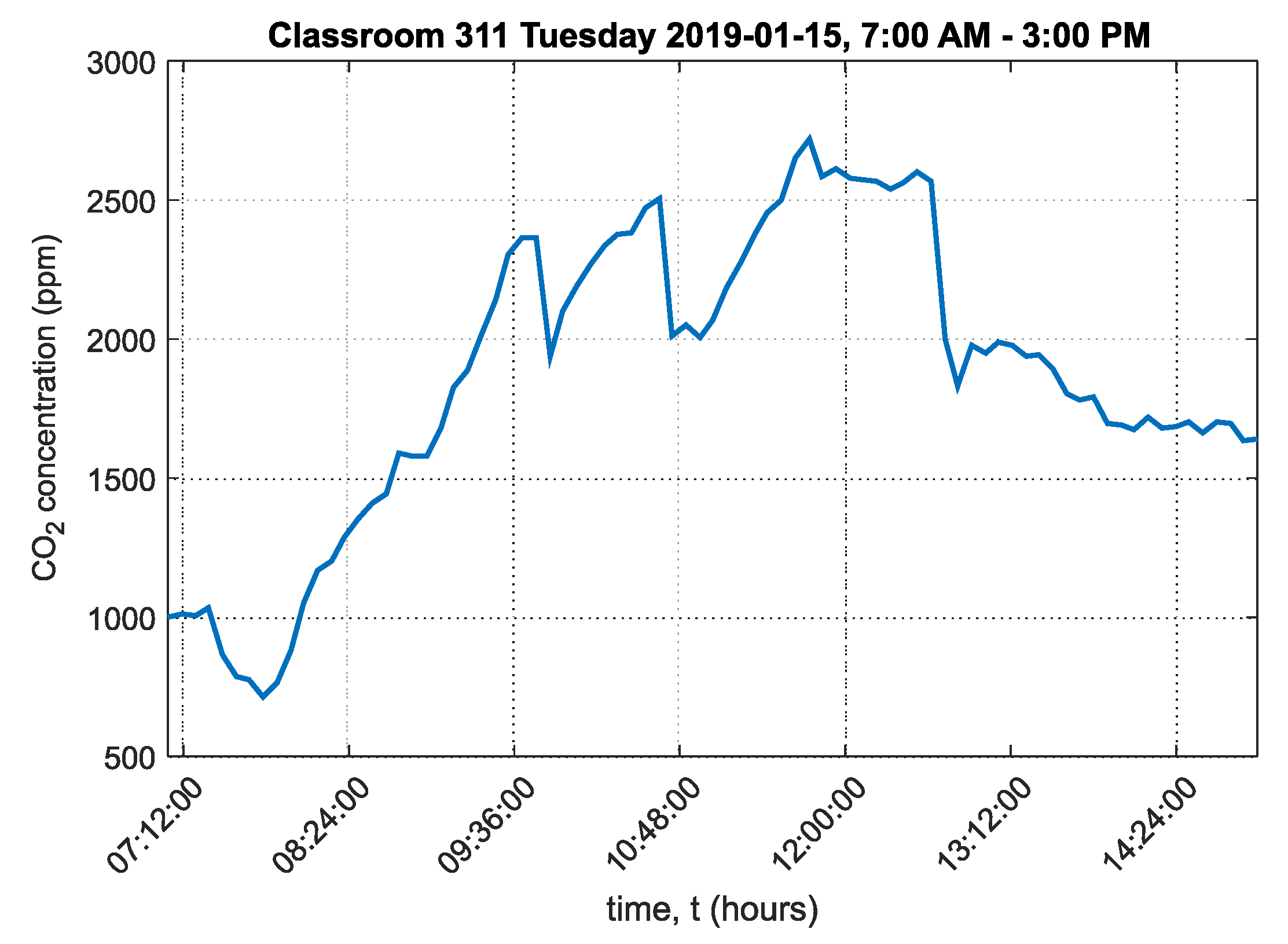
| 311 | 1867 | 716 | 2719 | 537 |
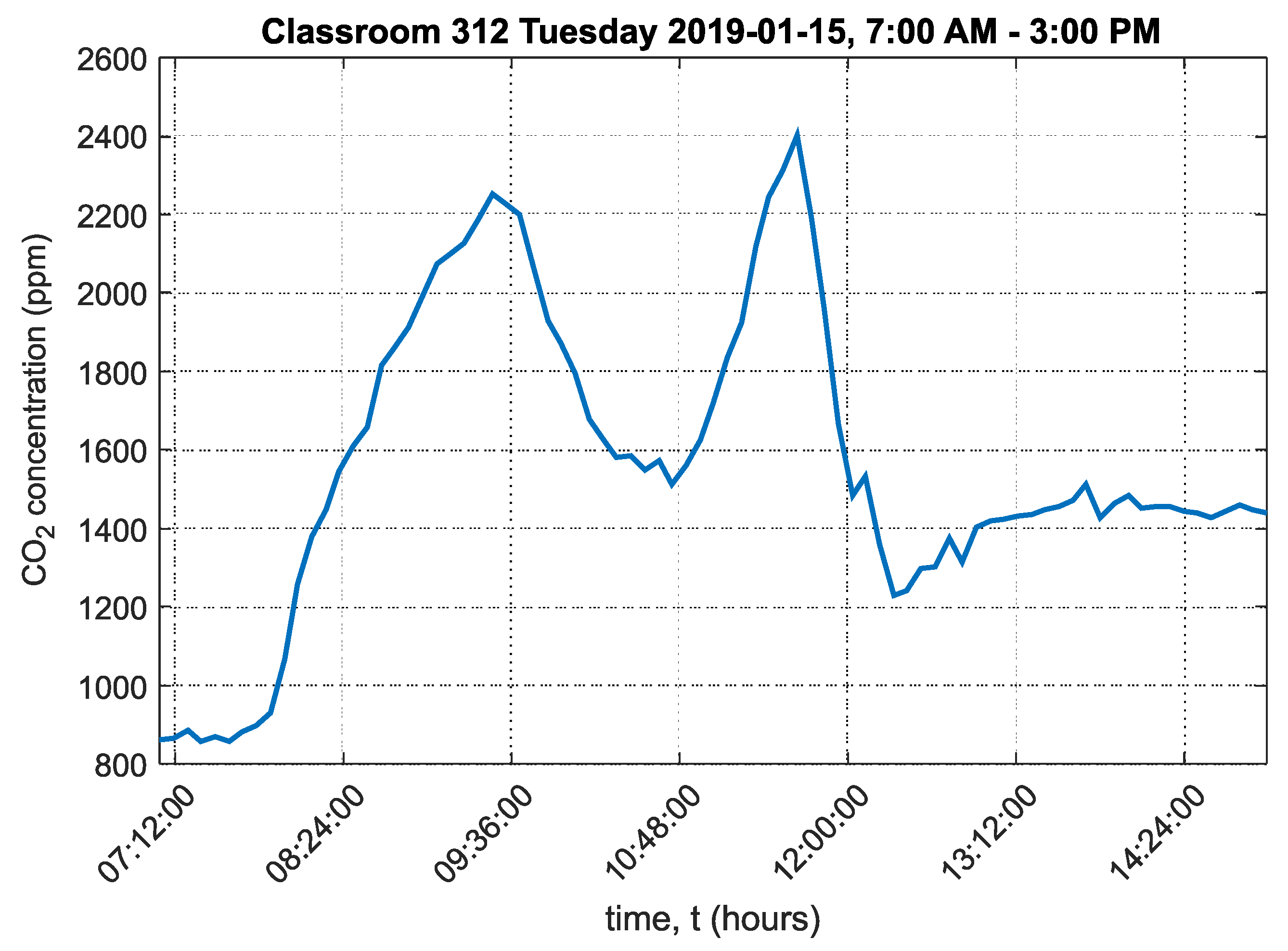
| 312 | 1567 | 855 | 2402 | 385 |
| 313 | 1508 | 671 | 3263 | 635 |
| Room Number | Variation (ppm2) | median (ppm) | under 1500 ppm (%) | |
| 311 | 288,068 | 1941 | 21 | |
| 312 | 148,281 | 1484 | 52 | |
| 313 | 403,594 | 1506 | 50 |
© 2020 by the authors. Licensee MDPI, Basel, Switzerland. This article is an open access article distributed under the terms and conditions of the Creative Commons Attribution (CC BY) license (http://creativecommons.org/licenses/by/4.0/).
Share and Cite
Pieš, M.; Hájovský, R.; Velička, J. Design, Implementation and Data Analysis of an Embedded System for Measuring Environmental Quantities. Sensors 2020, 20, 2304. https://doi.org/10.3390/s20082304
Pieš M, Hájovský R, Velička J. Design, Implementation and Data Analysis of an Embedded System for Measuring Environmental Quantities. Sensors. 2020; 20(8):2304. https://doi.org/10.3390/s20082304
Chicago/Turabian StylePieš, Martin, Radovan Hájovský, and Jan Velička. 2020. "Design, Implementation and Data Analysis of an Embedded System for Measuring Environmental Quantities" Sensors 20, no. 8: 2304. https://doi.org/10.3390/s20082304
APA StylePieš, M., Hájovský, R., & Velička, J. (2020). Design, Implementation and Data Analysis of an Embedded System for Measuring Environmental Quantities. Sensors, 20(8), 2304. https://doi.org/10.3390/s20082304