Using the Decomposition-Based Multi-Objective Evolutionary Algorithm with Adaptive Neighborhood Sizes and Dynamic Constraint Strategies to Retrieve Atmospheric Ducts

 , ,
, ,
Abstract
1. Introduction
2. Basic Concepts of Multi-Objective Optimization and Evaluation Metrics
2.1. Definition of Multi-Objective Optimization
2.2. Evaluation Metrics
2.3. Hypervolume
2.4. Inverted Generational Distance
2.5. Average Hausdorff Distance
3. MOEA/D Framework and Improvement
3.1. Basic Framework
3.2. Improvement
3.2.1. Adaptive Neighborhood Sizes
3.2.2. Adaptive Constraints Approach
4. Test Results
4.1. Results and Discussion of the Classical Test Functions
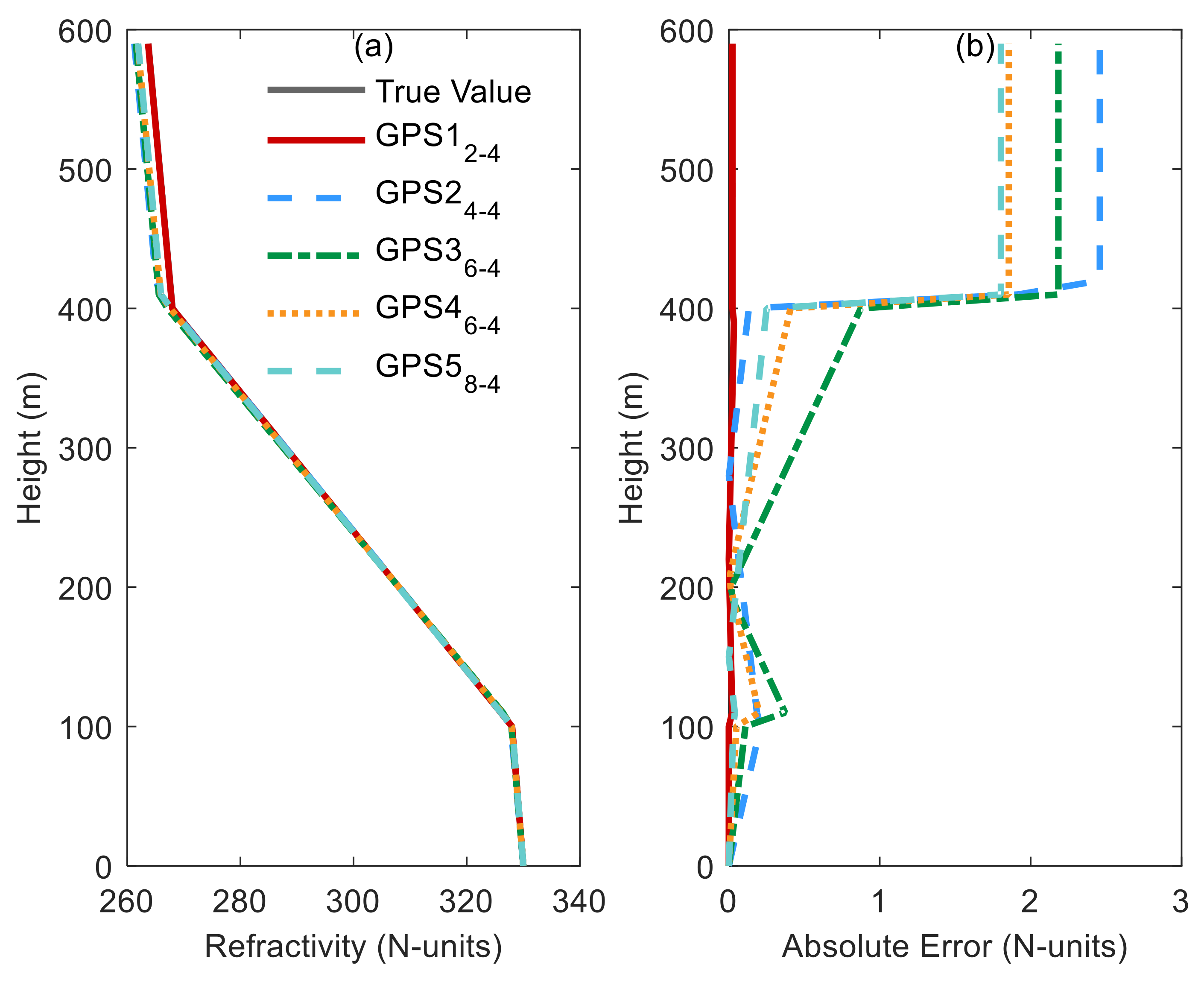
4.2. Results and Discussion of the Joint Inversion of Atmospheric Ducts Problem
5. Conclusions
Author Contributions
Funding
Conflicts of Interest
References
- Kou, J.; Xiong, S.; Fang, Z.; Zong, X.; Chen, Z. Multiobjective Optimization of Evacuation Routes in Stadium Using Superposed Potential Field Network Based ACO. Comput. Intel. Neurosc. 2013. [Google Scholar] [CrossRef]
- Lygoe, R.J.; Cary, M.; Fleming, P.J. A Real-World Application of a Many-Objective Optimisation Complexity Reduction Process. In Evolutionary Multi-Criterion Optimization, Emo 2013; Purshouse, R.C., Fleming, P.J., Fonesca, C.M., Greco, S., Shaw, J., Eds.; Springer Science and Business Media LLC: Berlin, Germany, 2013; Volume 7811, pp. 641–655. [Google Scholar]
- Trivedi, A.; Srinivasan, D.; Pal, K.; Saha, C.; Reindl, T. Enhanced Multiobjective Evolutionary Algorithm Based on Decomposition for Solving the Unit Commitment Problem. IEEE Trans. Ind. Inform. 2015, 11, 1346–1357. [Google Scholar] [CrossRef]
- Miettinen, K. Nonlinear Multiobjective Optimization. In International Series in Operations Research & Management Science; Springer: Berlin, Germany, 1998; Volume 12. [Google Scholar]
- Hanne, T. Global Multiobjective Optimization Using Evolutionary Algorithms. J. Heuristics. 2000, 6, 347–360. [Google Scholar] [CrossRef]
- Pradhan, P.M.; Panda, G. Pareto optimization of cognitive radio parameters using multiobjective evolutionary algorithms and fuzzy decision making. Swarm Evol. Comput. 2012, 7, 7–20. [Google Scholar] [CrossRef]
- Jin, Y.; Sendhoff, B. Pareto-Based Multiobjective Machine Learning: An Overview and Case Studies. IEEE Trans. Syst. Man Cybern 2008, 38, 397–415. [Google Scholar]
- Beume, N.; Naujoks, B.; Emmerich, M. SMS-EMOA: Multiobjective selection based on dominated hypervolume. Eur. J. Oper. Res. 2007, 181, 1653–1669. [Google Scholar] [CrossRef]
- Debels, D.; Vanhoucke, M. A decomposition-based genetic algorithm for the resource-constrained project-scheduling problem. Oper. Res. 2007, 55, 457–469. [Google Scholar] [CrossRef]
- Zitzler, E.; Laumanns, M.; Thiele, L. SPEA2: Improving the Strength Pareto Evolutionary Algorithm for Multiobjective Optimization. In Proceedings of the EUROGEN’2001, Athens, Greece, 19–21 September 2001; Volume 3242. [Google Scholar]
- Diaz-Manriquez, A.; Toscano, G.; Hugo Barron-Zambrano, J.; Tello-Leal, E. R2-Based Multi/Many-Objective Particle Swarm Optimization. Comput. Int. Neurosc. 2016. [Google Scholar] [CrossRef]
- Schuetze, O.; Esquivel, X.; Lara, A.; Coello Coello, C.A. Using the Averaged Hausdorff Distance as a Performance Measure in Evolutionary Multiobjective Optimization. IEEE Trans. Evolut. Comput. 2012, 16, 504–522. [Google Scholar] [CrossRef]
- Guo, X. A New Decomposition Many-Objective Evolutionary Algorithm Based on—Efficiency Order Dominance. In Advances in Intelligent Information Hiding and Multimedia Signal Processing; Pan, J.S., Tsai, P.W., Watada, J., Jain, L.C., Eds.; Springer: Cham, Switzerland, 2018; Volume 81, pp. 242–249. [Google Scholar]
- Li, K.; Wang, R.; Zhang, T.; Ishibuchi, H. Evolutionary Many-Objective Optimization: A Comparative Study of the State-of-the-Art. IEEE Access 2018, 6, 26194–26214. [Google Scholar] [CrossRef]
- Zhao, S.-Z.; Suganthan, P.N.; Zhang, Q. Decomposition-Based Multiobjective Evolutionary Algorithm with an Ensemble of Neighborhood Sizes. IEEE Trans. Evolut. Comput. 2012, 16, 442–446. [Google Scholar] [CrossRef]
- Martin, A.; Schutze, O. Pareto Tracer: A predictor-corrector method for multi-objective optimization problems. Eng. Optim. 2018, 50, 516–536. [Google Scholar] [CrossRef]
- Janssens, J.; Sorensen, K.; Janssens, G.K. Studying the influence of algorithmic parameters and instance characteristics on the performance of a multiobjective algorithm using the Promethee method. Cybern. Syst. 2019, 50, 444–464. [Google Scholar] [CrossRef]
- Yang, Y.; Huang, M.; Wang, Z.; Zhu, Q. Dual-information-based evolution and dual-selection strategy in evolutionary multiobjective optimization. Soft Comput. 2019. [Google Scholar] [CrossRef]
- Hernandez, C.; Schutze, O.; Sun, J.-Q. Global Multi-objective Optimization by Means of Cell Mapping Techniques. In Evolve—A Bridge between Probability, Set Oriented Numerics and Evolutionary Computation Vii; Emmerich, M., Deutz, A., Schutze, O., Legrand, P., Tantar, E., Tantar, A.A., Eds.; Springer: Berlin, Germany, 2017; Volume 662, pp. 25–56. [Google Scholar]
- Dellnitz, M.; Schutze, O.; Hestermeyer, T. Covering Pareto sets by multilevel subdivision techniques. J. Optim. Theory Appl. 2005, 124, 113–136. [Google Scholar] [CrossRef]
- Schuetze, O.; Coello Coello, C.A.; Mostaghim, S.; Talbi, E.-g.; Dellnitz, M. Hybridizing evolutionary strategies with continuation methods for solving multi-objective problems. Eng. Optim. 2008, 40, 383–402. [Google Scholar] [CrossRef]
- Wang, L.; Zhang, Q.; Zhou, A.; Gong, M.; Jiao, L. Constrained Subproblems in a Decomposition-Based Multiobjective Evolutionary Algorithm. IEEE Trans. Evolut. Comput. 2016, 20, 475–480. [Google Scholar] [CrossRef]
- Mai, Y.; Sheng, Z.; Shi, H.; Liao, Q.; Zhang, W. Spatiotemporal Distribution of Atmospheric Ducts in Alaska and Its Relationship with the Arctic Vortex. Int. J. Antennas Propag. 2020, 9673289. [Google Scholar] [CrossRef]
- Zhao, X.; Sheng, Z.; Li, J.; Yu, H.; Wei, K. Determination of the “wave turbopause” using a numerical differentiation method. J. Geophys. Res. Atmos. 2019, 124. [Google Scholar] [CrossRef]
- He, Y.; Sheng, Z.; He, M. Spectral Analysis of Gravity Waves from Near Space High-Resolution Balloon Data in Northwest China. Atmosphere 2020, 11, 133. [Google Scholar] [CrossRef]
- Sheng, Z.; Zhou, L.; He, Y. Retrieval and Analysis of the Strongest Mixed Layer in the Troposphere. Atmosphere 2020, 11, 264. [Google Scholar] [CrossRef]
- Shen, Y.; Sun, Y.; Camargo, S.; Zhong, Z. A Quantitative Method to Evaluate Tropical Cyclone Tracks in Climate Models. J. Atmos. Ocean. Technol. 2018, 35, 1807–1818. [Google Scholar] [CrossRef]
- Chang, S.; Sheng, Z.; Du, H.; Ge, W.; Zhang, W. A channel selection method for hyperspectral atmospheric infrared sounders based on layering. Atmos. Meas. Tech. 2020, 13, 629–644. [Google Scholar] [CrossRef]
- He, Y.; Sheng, Z.; He, M. The First Observation of Turbulence in Northwestern China by a Near-Space High-Resolution Balloon Sensor. Sensors 2020, 20, 677. [Google Scholar] [CrossRef] [PubMed]
- Sheng, Z.; Fang, H.-X. Monitoring of ducting by using a ground-based GPS receiver. Chin. Phys. B 2013, 22. [Google Scholar] [CrossRef]
- Zhang, Q.; Liu, W.; Li, H.; IEEE. The Performance of a New Version of MOEA/D on CEC09 Unconstrained MOP Test Instances. In Proceedings of the Congress on Evolutionary Computation, Trondheim, Norway, 18–21 May 2009; pp. 203–208. [Google Scholar] [CrossRef]
- Liao, Q.; Sheng, Z.; Shi, H.; Zhang, L.; Zhou, L.; Ge, W.; Long, Z. A Comparative Study on Evolutionary Multi-objective Optimization Algorithms Estimating Surface Duct. Sensors 2018, 18. [Google Scholar] [CrossRef]
- Shen, P.; Braham, W.; Yi, Y.; Eaton, E. Rapid multi-objective optimization with multi-year future weather condition and decision-making support for building retrofit. Energy 2019, 172, 892–912. [Google Scholar] [CrossRef]
- Pasquier, P.; Zarrella, A.; Marcotte, D. A multi-objective optimization strategy to reduce correlation and uncertainty for thermal response test analysis. Geothermics 2019, 79, 176–187. [Google Scholar] [CrossRef]
- Knowles, J.D.; Thiele, L.; Zitzler, E. A Tutorial on the Performance Assessment of Stochastic Multiobjective Optimizers; TIK: Guanajuato, Mexico, 2006. [Google Scholar]
- Zitzler, E.; Thiele, L. Multiobjective Evolutionary Algorithms: A Comparative Case Study and the Strength Pareto Approach. IEEE Trans. Evolut. Comput. 1999, 3, 257–271. [Google Scholar] [CrossRef]
- Ishibuchi, H.; Masuda, H.; Tanigaki, Y.; Nojima, Y.; IEEE. Difficulties in Specifying Reference Points to Calculate the Inverted Generational Distance for Many-Objective Optimization Problems. In Proceedings of the 2014 IEEE Symposium on Computational Intelligence in Multi-Criteria Decision-Making (MCDM), Orlando, FL, USA, 9–12 December 2014; pp. 170–177. [Google Scholar] [CrossRef]
- Qiao, J.; Zhou, H.; Yang, C.; Yang, S. A decomposition-based multiobjective evolutionary algorithm with angle-based adaptive penalty. Appl. Soft Comput. 2019, 74, 190–205. [Google Scholar] [CrossRef]
- Qi, Y.; Ma, X.; Liu, F.; Jiao, L.; Sun, J.; Wu, J. MOEA/D with Adaptive Weight Adjustment. Evol. Comput. 2014, 22, 231–264. [Google Scholar] [CrossRef]
- Li, X.; Zhang, H.; Song, S. MOEA/D with the online agglomerative clustering based self-adaptive mating restriction strategy. Neurocomputing 2019, 339, 77–93. [Google Scholar] [CrossRef]
- Li, H.; Landa-Silva, D. An Adaptive Evolutionary Multi-Objective Approach Based on Simulated Annealing. Evol. Comput. 2011, 19, 561–595. [Google Scholar] [CrossRef] [PubMed]
- Li, H.; Zhang, Q. Multiobjective Optimization Problems with Complicated Pareto Sets, MOEA/D and NSGA-II. IEEE Trans. Evolut. Comput. 2009, 13, 284–302. [Google Scholar] [CrossRef]
- Li, K.; Kwong, S.; Zhang, Q.; Deb, K. Interrelationship-Based Selection for Decomposition Multiobjective Optimization. IEEE Trans. Cybern. 2015, 45, 2076–2088. [Google Scholar] [CrossRef] [PubMed]
- Mashwani, W.K.; Salhi, A. Multiobjective evolutionary algorithm based on multimethod with dynamic resources allocation. Appl. Soft Comput. 2016, 39, 292–309. [Google Scholar] [CrossRef]
- Das, S.; Suganthan, P.N. Differential Evolution: A Survey of the State-of-the-Art. IEEE Trans. Evolut. Comput. 2011, 15, 4–31. [Google Scholar] [CrossRef]
- Galvan, E.; Malak, R.J.; Hartl, D.J.; Baur, J.W. Performance assessment of a multi-objective parametric optimization algorithm with application to a multi-physical engineering system. Struct. Multidiscip. Optim. 2018, 58, 489–509. [Google Scholar] [CrossRef]
- Whitney, W.; Rana, S.; Dzubera, J.; Mathias, K.E. Evaluating Evolutionary Algorithms. Artif. Intell. 1996, 84, 357–358. [Google Scholar] [CrossRef]
- Kalyanmoy, D. Multi-Objective Optimization Using Evolutionary Algorithms; Wiley: Chichester, UK, 2011; p. 16. [Google Scholar] [CrossRef]
- Fonseca, C.; Knowles, J.; Thiele, L.; Zitzler, E. A tutorial on the performance assessment of stochastic multiobjective optimizers. Tik Rep. 2006, 214, 327–332. [Google Scholar]
- Storn, R.; Price, K. Differential Evolution—A Simple and Efficient Heuristic for global Optimization over Continuous Spaces. J. Glob. Optim. 1997, 11, 341–359. [Google Scholar] [CrossRef]
- Liao, Q.; Sheng, Z.; Shi, H.; Xiang, J.; Yu, H. Estimation of Surface Duct Using Ground-Based GPS Phase Delay and Propagation Loss. Remote Sens. 2018, 10. [Google Scholar] [CrossRef]


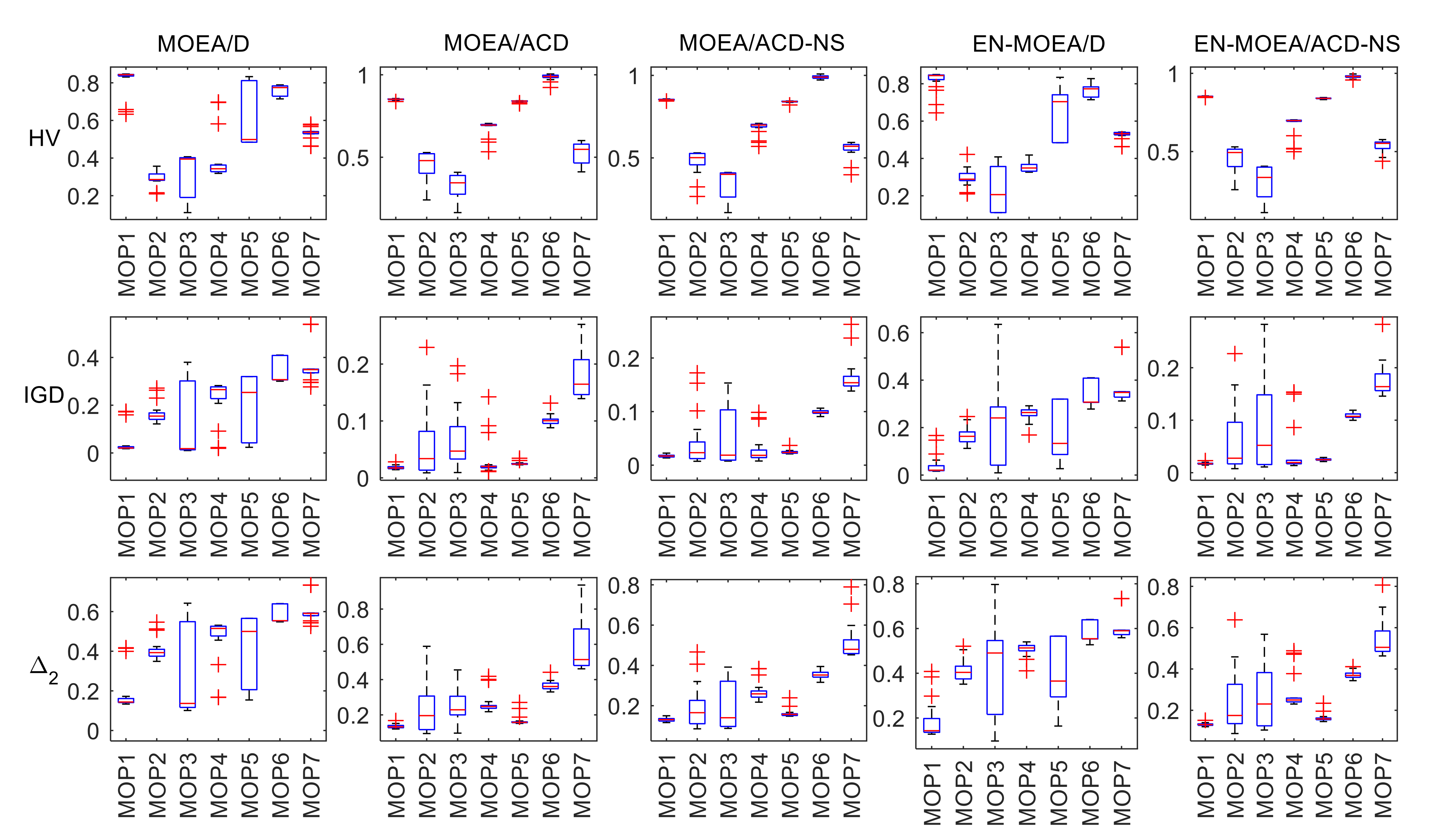
| Functions | Mean (SD) | ||||
|---|---|---|---|---|---|
| MOEA/D | MOEA/ACD | MOEA/ACD-NS | EN-MOEA/D | EN-MOEA/ACD-NS | |
| UF1 | 0.6999(0.0729) | 0.7239(0.0562) | 0.7551(0.0790) | 0.6706(0.0629) | 0.7509(0.0507) |
| UF2 | 0.7730(0.0386) | 0.8347(0.0077) | 0.8318(0.0156) | 0.7629(0.0369) | 0.8308(0.0144) |
| UF3 | 0.4534(0.0229) | 0.6260(0.0919) | 0.5630(0.0948) | 0.4514(0.0267) | 0.5933(0.0949) |
| UF4 | 0.3946(0.0133) | 0.4033(0.0110) | 0.4090(0.0106) | 0.4036(0.0105) | 0.3984(0.0124) |
| UF5 | 0.2068(0.0850) | 0.0717(0.0694) | 0.1816(0.0810) | 0.2173(0.0882) | 0.0589(0.0599) |
| UF6 | 0.1966(0.1090) | 0.2960(0.0963) | 0.3237(0.0744) | 0.2681(0.1043) | 0.3242(0.0786) |
| UF7 | 0.4473(0.2176) | 0.6540(0.0822) | 0.6502(0.0837) | 0.4712(0.1772) | 0.5806(0.1508) |
| UF8 | 0.4129(0.0876) | 0.3838(0.0944) | 0.4177(0.0508) | 0.3154(0.1579) | 0.3977(0.0468) |
| UF9 | 0.7864(0.0322) | 0.7476(0.0577) | 0.7443(0.0768) | 0.7871(0.0376) | 0.7434(0.0647) |
| UF10 | 0.1440(0.0211) | 0.0079(0.0098) | 0.0438(0.0332) | 0.1298(0.0309) | 0.0042(0.0111) |
| MOP1 | 0.8127(0.0722) | 0.8509(0.0043) | 0.8524(0.0033) | 0.8173(0.0567) | 0.8522(0.0024) |
| MOP2 | 0.2888(0.0417) | 0.4545(0.0777) | 0.4769(0.0713) | 0.2971(0.0513) | 0.4560(0.0826) |
| MOP3 | 0.3121(0.1088) | 0.3261(0.0775) | 0.3440(0.0824) | 0.2381(0.1153) | 0.3054(0.1105) |
| MOP4 | 0.3865(0.1200) | 0.6792(0.0455) | 0.6808(0.0414) | 0.3520(0.0238) | 0.6656(0.0697) |
| MOP5 | 0.6326(0.1657) | 0.8391(0.0046) | 0.8404(0.0052) | 0.6293(0.1383) | 0.8397(0.0033) |
| MOP6 | 0.7570(0.0295) | 0.9858(0.0188) | 0.9900(0.0093) | 0.7612(0.0326) | 0.9787(0.0092) |
| MOP7 | 0.5296(0.0330) | 0.5294(0.0617) | 0.5536(0.0497) | 0.5258(0.0230) | 0.5373(0.0376) |
| Functions | Mean (SD) | ||||
|---|---|---|---|---|---|
| MOEA/D | MOEA/ACD | MOEA/ACD-NS | EN-MOEA/D | EN-MOEA/ACD-NS | |
| UF1 | 0.1593(0.0835) | 0.0983(0.0522) | 0.0801(0.0613) | 0.2173(0.0819) | 0.0856(0.0549) |
| UF2 | 0.1224(0.0614) | 0.0317(0.0090) | 0.0376(0.0217) | 0.1416(0.0572) | 0.0346(0.0169) |
| UF3 | 0.3200(0.0063) | 0.1752(0.0502) | 0.2141(0.0441) | 0.3235(0.0062) | 0.1963(0.0514) |
| UF4 | 0.0864(0.0081) | 0.0812(0.0072) | 0.0778(0.0069) | 0.0804(0.0068) | 0.0842(0.0078) |
| UF5 | 0.4804(0.0864) | 0.6216(0.1270) | 0.4874(0.0968) | 0.4762(0.1002) | 0.6545(0.1489) |
| UF6 | 0.6001(0.1374) | 0.4078(0.1773) | 0.3846(0.1399) | 0.5395(0.1644) | 0.3950(0.1558) |
| UF7 | 0.2778(0.2576) | 0.0422(0.0841) | 0.0424(0.0831) | 0.2368(0.1981) | 0.1213(0.1612) |
| UF8 | 0.2094(0.1154) | 0.2194(0.1021) | 0.1833(0.0323) | 0.3608(0.2347) | 0.1959(0.0309) |
| UF9 | 0.1814(0.0211) | 0.2002(0.0264) | 0.1992(0.0411) | 0.1845(0.0223) | 0.2019(0.0365) |
| UF10 | 0.6282(0.0903) | 0.8355(0.1020) | 0.6488(0.1032) | 0.6323(0.0972) | 0.9867(0.2256) |
| MOP1 | 0.0436(0.0541) | 0.0182(0.0032) | 0.0172(0.0024) | 0.0415(0.0436) | 0.0173(0.0019) |
| MOP2 | 0.1660(0.0419) | 0.0593(0.0613) | 0.0417(0.0474) | 0.1667(0.0381) | 0.0600(0.0665) |
| MOP3 | 0.1395(0.1585) | 0.0652(0.0543) | 0.0506(0.0515) | 0.2142(0.1790) | 0.0850(0.0864) |
| MOP4 | 0.2288(0.0832) | 0.0311(0.0335) | 0.0296(0.0275) | 0.2580(0.0286) | 0.0419(0.0499) |
| MOP5 | 0.1904(0.1363) | 0.0251(0.0028) | 0.0244(0.0034) | 0.1934(0.1200) | 0.0250(0.0021) |
| MOP6 | 0.3521(0.0526) | 0.1015(0.0089) | 0.0990(0.0038) | 0.3460(0.0530) | 0.1087(0.0052) |
| MOP7 | 0.3653(0.0780) | 0.1819(0.0424) | 0.1652(0.0313) | 0.3580(0.0636) | 0.1773(0.0327) |
| Functions | Mean (SD) | ||||
|---|---|---|---|---|---|
| MOEA/D | MOEA/ACD | MOEA/ACD-NS | EN-MOEA/D | EN-MOEA/ACD-NS | |
| UF1 | 0.3849(0.1081) | 0.3128(0.0836) | 0.2723(0.0946) | 0.4583(0.0877) | 0.2850(0.0861) |
| UF2 | 0.3373(0.0955) | 0.1766(0.0242) | 0.1877(0.0496) | 0.3670(0.0857) | 0.1822(0.0386) |
| UF3 | 0.5656(0.0056) | 0.4158(0.0584) | 0.4604(0.0473) | 0.5688(0.0054) | 0.4394(0.0584) |
| UF4 | 0.3032(0.0141) | 0.2935(0.0120) | 0.2868(0.0121) | 0.2924(0.0115) | 0.2990(0.0135) |
| UF5 | 0.6905(0.0619) | 0.7902(0.0913) | 0.7020(0.0730) | 0.6867(0.0702) | 0.8131(0.0975) |
| UF6 | 0.7698(0.0894) | 0.6405(0.1223) | 0.6183(0.0997) | 0.7277(0.1025) | 0.6213(0.1203) |
| UF7 | 0.4494(0.2826) | 0.1739(0.1259) | 0.1818(0.1270) | 0.4332(0.2276) | 0.2764(0.2182) |
| UF8 | 0.5201(0.0999) | 0.6114(0.0888) | 0.5866(0.0998) | 0.6153(0.1617) | 0.6106(0.0988) |
| UF9 | 0.4886(0.0335) | 0.6215(0.0399) | 0.6274(0.0580) | 0.4863(0.0395) | 0.6353(0.0550) |
| UF10 | 0.7905(0.0586) | 1.0085(0.1498) | 0.8356(0.1440) | 0.7929(0.0609) | 1.1933(0.3305) |
| MOP1 | 0.1859(0.0974) | 0.1345(0.0114) | 0.1308(0.0089) | 0.1863(0.0845) | 0.1314(0.0071) |
| MOP2 | 0.4073(0.0537) | 0.2351(0.1347) | 0.1907(0.1066) | 0.4107(0.0512) | 0.2344(0.1516) |
| MOP3 | 0.3052(0.2278) | 0.2451(0.1033) | 0.1966(0.1139) | 0.4235(0.2232) | 0.2670(0.1464) |
| MOP4 | 0.4674(0.1119) | 0.2680(0.0605) | 0.2722(0.0470) | 0.5071(0.0298) | 0.2870(0.0882) |
| MOP5 | 0.4005(0.1777) | 0.1683(0.0305) | 0.1619(0.0210) | 0.4156(0.1476) | 0.1630(0.0198) |
| MOP6 | 0.5919(0.0441) | 0.3658(0.0255) | 0.3546(0.0204) | 0.5866(0.0446) | 0.3720(0.0166) |
| MOP7 | 0.6015(0.0605) | 0.5935(0.1536) | 0.5146(0.0892) | 0.5965(0.0488) | 0.5452(0.0885) |
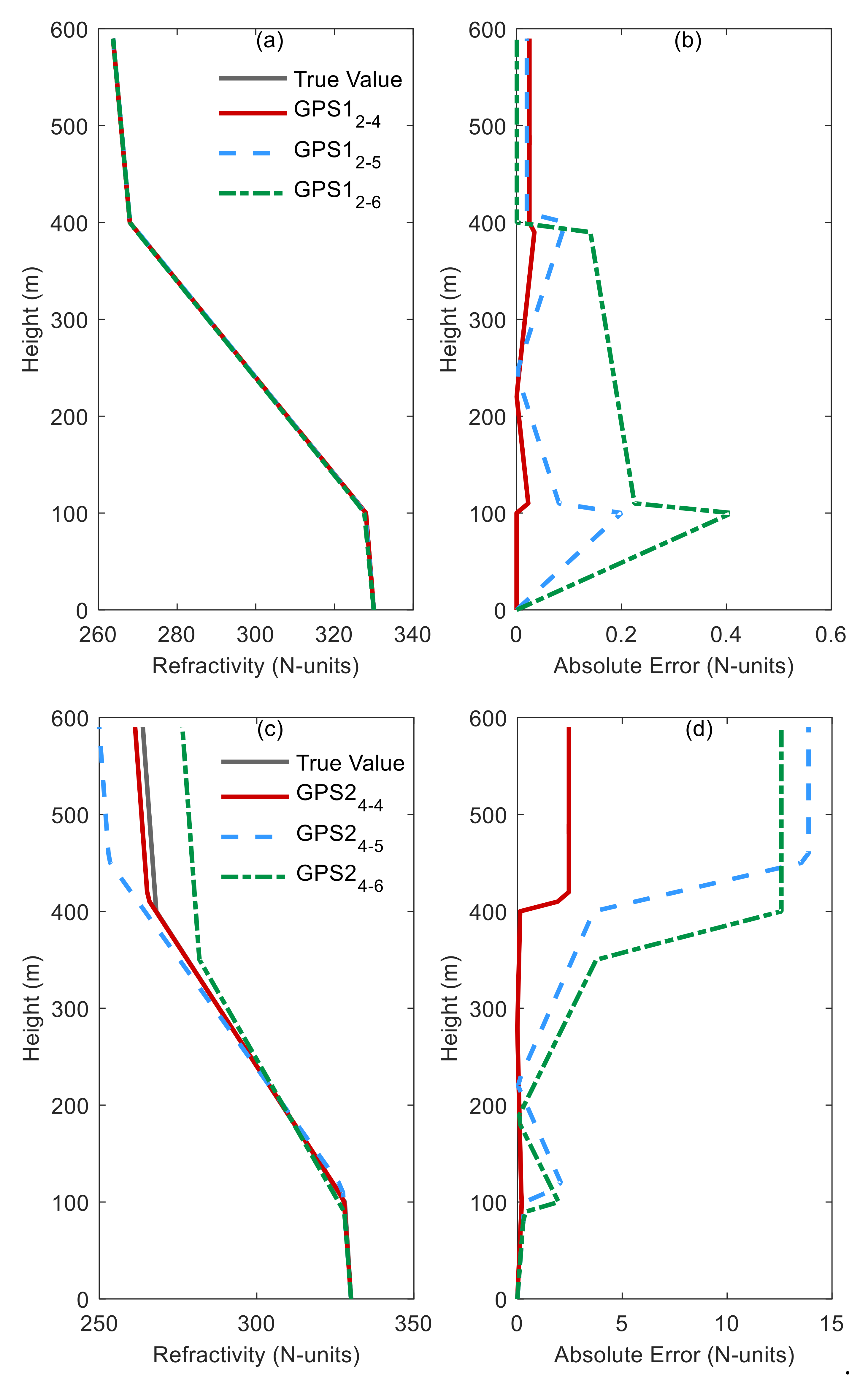
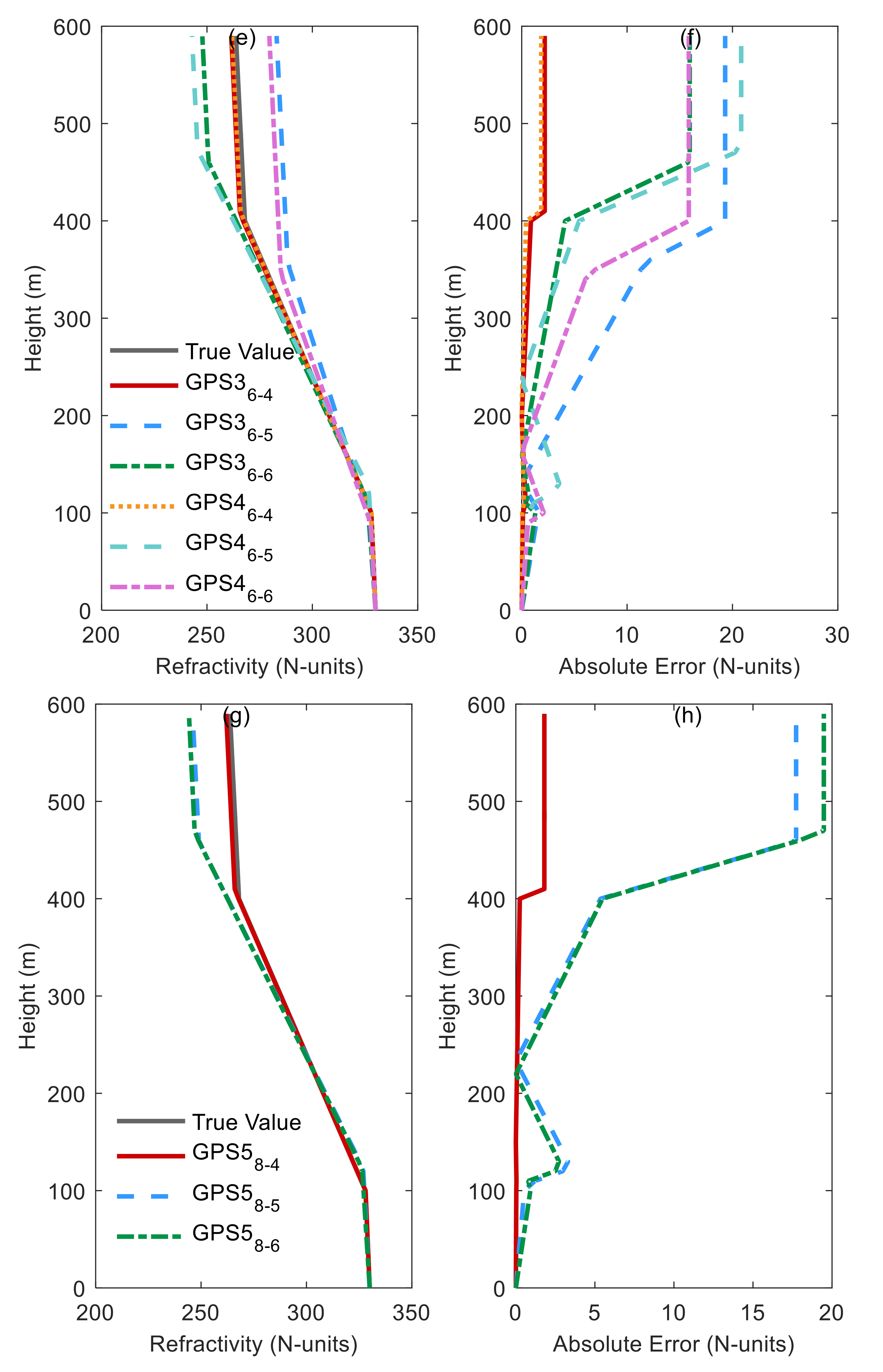
| Problems | M | D | Inversion Slope c1 | Height h1 | Inversion Slope c2 | Height h2 | Δ2 |
|---|---|---|---|---|---|---|---|
| Simulated Results | - | - | 100 | 300 | −0.02 | −0.2 | - |
| GPS1 | 2 | 4 | 100.1342 (0.0065) | 299.8013 (0.0060) | 0.02 (0.0000) | 0.2002 (0.000) | 1.666 (0.1924) |
| GPS1 | 2 | 5 | 100.6387 (0.0091) | 299.7782 (0.0057) | 0.0220 (0.0000) | 0.1994 (0.0059) | 1.6453 (0.0965) |
| GPS1 | 2 | 6 | 101.0383 (0.0802) | 298.1824 (0.1055) | 0.0241 (0.0002) | 0.1997 (0.0002) | 1.7403 (0.1496) |
| GPS2 | 4 | 4 | 102.2753 (3.2614) | 310.7474 (20.0969) | 0.0221 (0.0018) | 0.2011 (0.0028) | 1.9413 (0.0727) |
| GPS2 | 4 | 5 | 114.3822 (12.0344) | 337.3833 (14.1259) | 0.0235 (0.0033) | 0.2204 (0.0163) | 2.8771 (0.0826) |
| GPS2 | 4 | 6 | 89.4901 (10.8181) | 260.8328 (12.1285) | 0.0235 (0.0047) | 0.1771 (0.0209) | 2.8869 (0.0657) |
| GPS3 | 6 | 4 | 102.8699 (10.8528) | 304.3318 (13.2847) | 0.0211 (0.0036) | 0.2043 (0.0165) | 2.2986 (0.0693) |
| GPS3 | 6 | 5 | 99.0262 (17.7310) | 257.8824 (8.6933) | 0.0354 (0.0190) | 0.1482 (0.0649) | 3.3573 (0.0729) |
| GPS3 | 6 | 6 | 112.3220 (16.0652) | 348.4416 (4.0524) | 0.0329 (0.0070) | 0.2170 (0.0289) | 3.7982 (0.1053) |
| GPS4 | 6 | 4 | 101.4928 (5.7184) | 306.5612 (15.5952) | 0.0205 (0.0033) | 0.2021 (0.0070) | 2.3387 (0.0482) |
| GPS4 | 6 | 5 | 124.9876 (14.0261) | 347.9198 (2.9298) | 0.0261 (0.0048) | 0.2334 (0.0215) | 3.3931 (0.0573) |
| GPS4 | 6 | 6 | 89.6128 (13.9242) | 256.1806 (7.1527) | 0.0265 (0.0062) | 0.1661 (0.0440) | 3.3632 (0.0622) |
| GPS5 | 8 | 4 | 100.1070 (0.1295) | 308.5910 (17.9959) | 0.0197 (0.0011) | 0.2010 (0.0017) | 2.5372 (0.0503) |
| GPS5 | 8 | 5 | 123.2109 (18.3929) | 335.7955 (28.5190) | 0.0253 (0.0038) | 0.2321 (0.0409) | 3.8360 (0.0680) |
| GPS5 | 8 | 6 | 122.6695 (16.0692) | 344.6790 (5.0537) | 0.0292 (0.0074) | 0.2304 (0.0218) | 3.7798 (0.0850) |
© 2020 by the authors. Licensee MDPI, Basel, Switzerland. This article is an open access article distributed under the terms and conditions of the Creative Commons Attribution (CC BY) license (http://creativecommons.org/licenses/by/4.0/).
Share and Cite
Mai, Y.; Shi, H.; Liao, Q.; Sheng, Z.; Zhao, S.; Ni, Q.; Zhang, W. Using the Decomposition-Based Multi-Objective Evolutionary Algorithm with Adaptive Neighborhood Sizes and Dynamic Constraint Strategies to Retrieve Atmospheric Ducts. Sensors 2020, 20, 2230. https://doi.org/10.3390/s20082230
Mai Y, Shi H, Liao Q, Sheng Z, Zhao S, Ni Q, Zhang W. Using the Decomposition-Based Multi-Objective Evolutionary Algorithm with Adaptive Neighborhood Sizes and Dynamic Constraint Strategies to Retrieve Atmospheric Ducts. Sensors. 2020; 20(8):2230. https://doi.org/10.3390/s20082230
Chicago/Turabian StyleMai, Yanbo, Hanqing Shi, Qixiang Liao, Zheng Sheng, Shuai Zhao, Qingjian Ni, and Wei Zhang. 2020. "Using the Decomposition-Based Multi-Objective Evolutionary Algorithm with Adaptive Neighborhood Sizes and Dynamic Constraint Strategies to Retrieve Atmospheric Ducts" Sensors 20, no. 8: 2230. https://doi.org/10.3390/s20082230
APA StyleMai, Y., Shi, H., Liao, Q., Sheng, Z., Zhao, S., Ni, Q., & Zhang, W. (2020). Using the Decomposition-Based Multi-Objective Evolutionary Algorithm with Adaptive Neighborhood Sizes and Dynamic Constraint Strategies to Retrieve Atmospheric Ducts. Sensors, 20(8), 2230. https://doi.org/10.3390/s20082230