Deep Learning to Unveil Correlations between Urban Landscape and Population Health †

 , and
, and
Abstract
1. Introduction
Background and Related Work
2. Materials and Methods
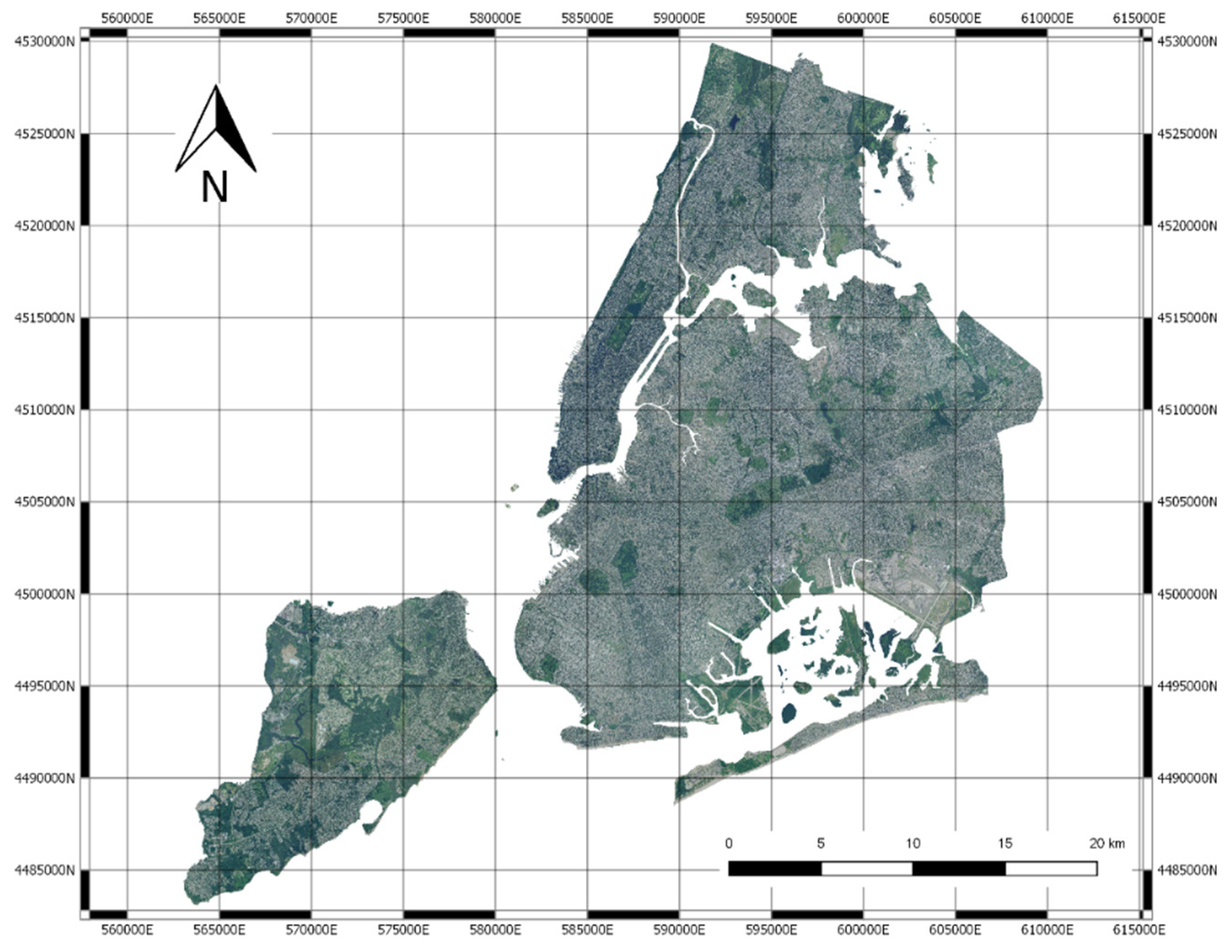
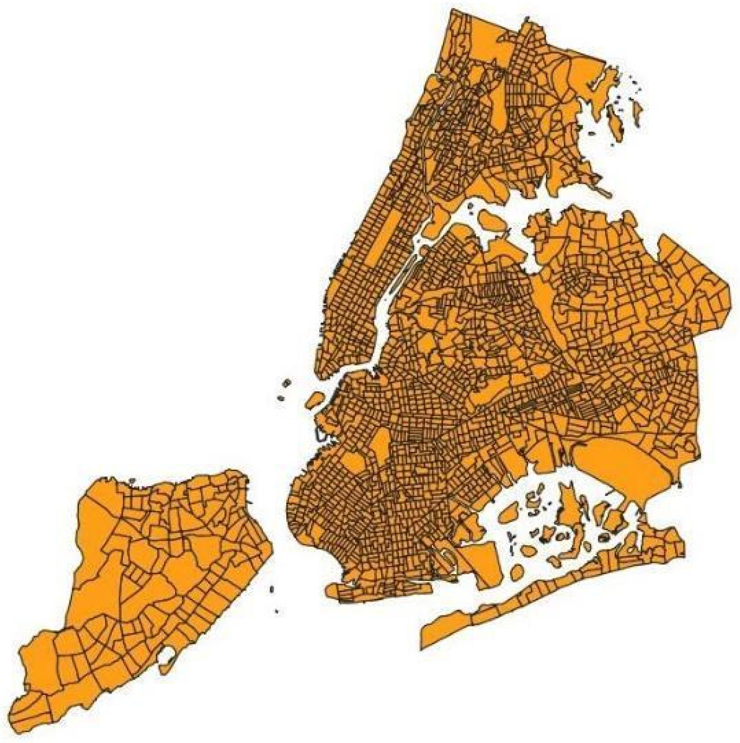
2.1. Data
2.2. The Data Analysis Pipeline
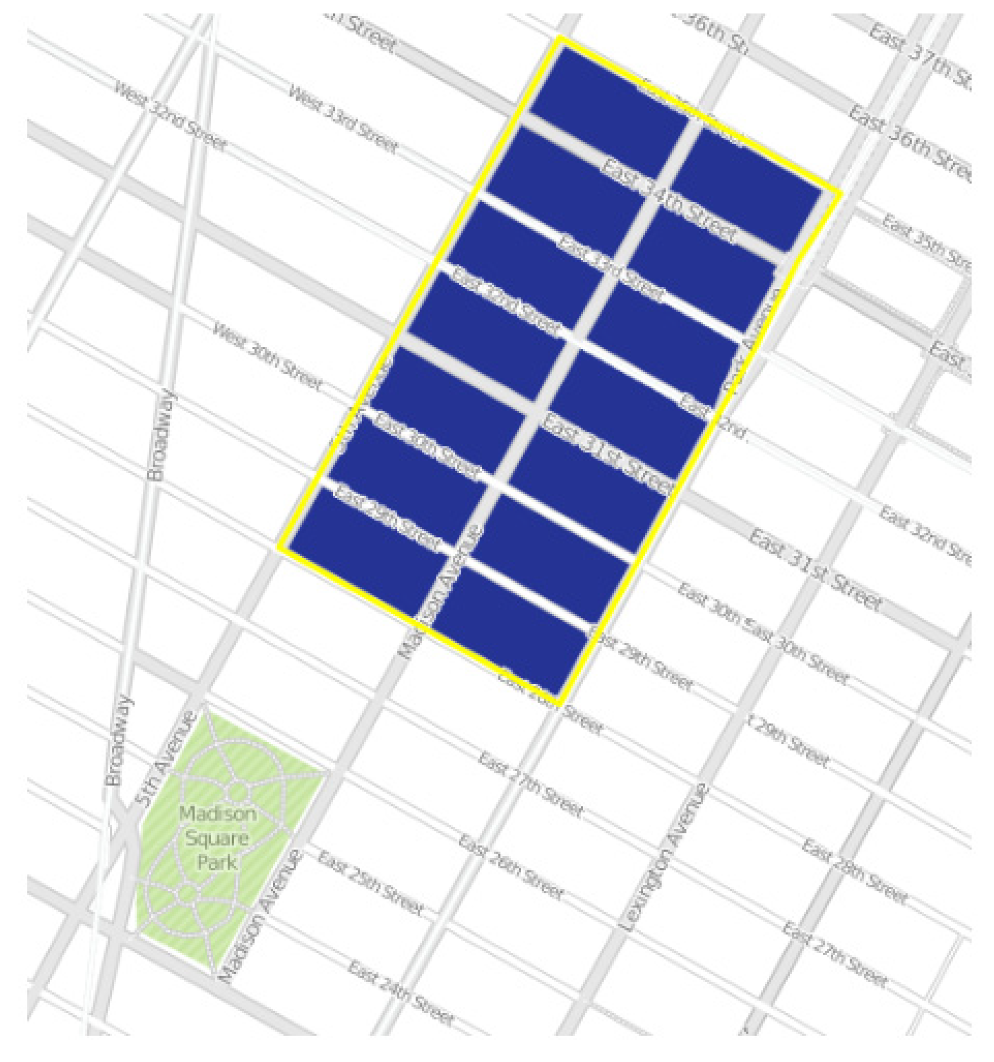
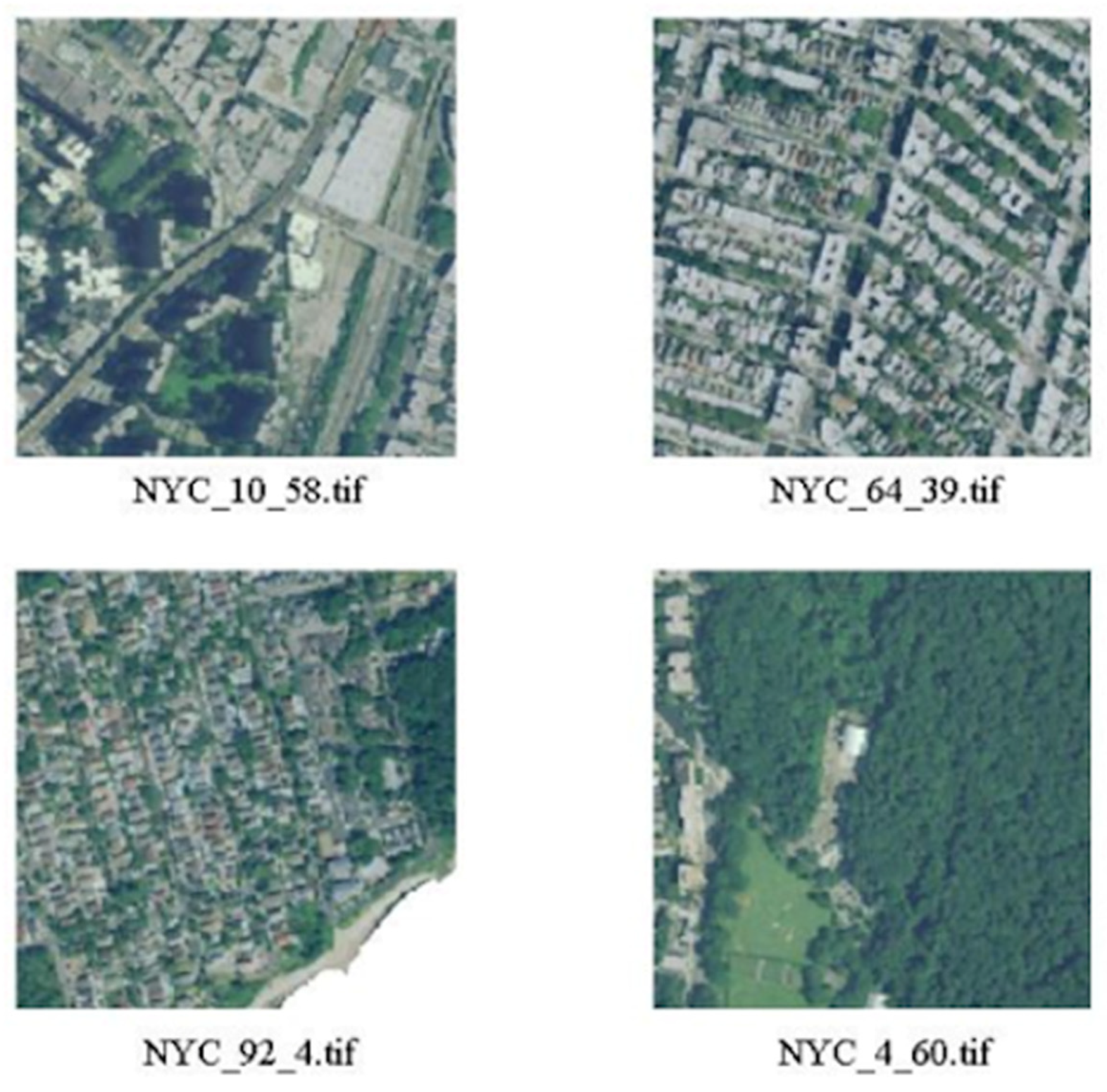
2.3. Image Blocks
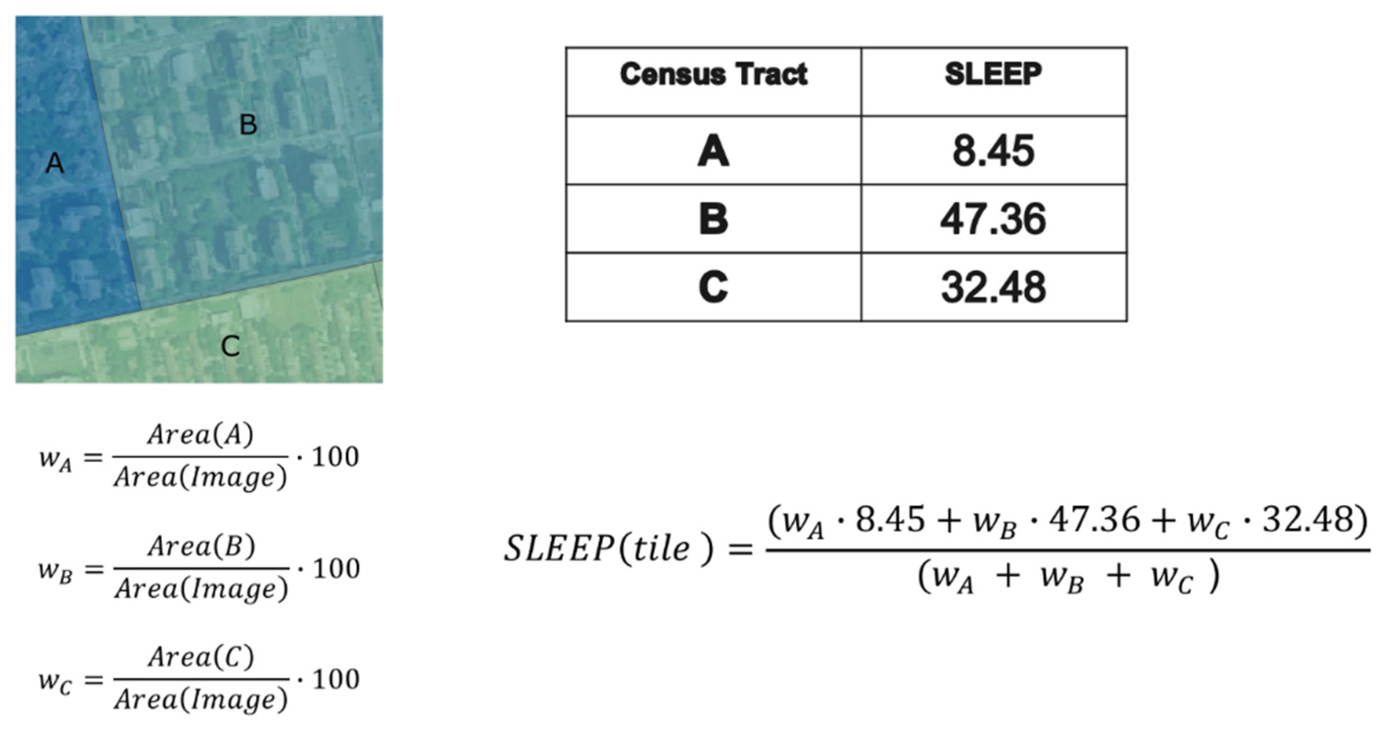
2.4. Estimation of Healthcare Indexes
2.5. Deep Neural Network Processing and Clustering
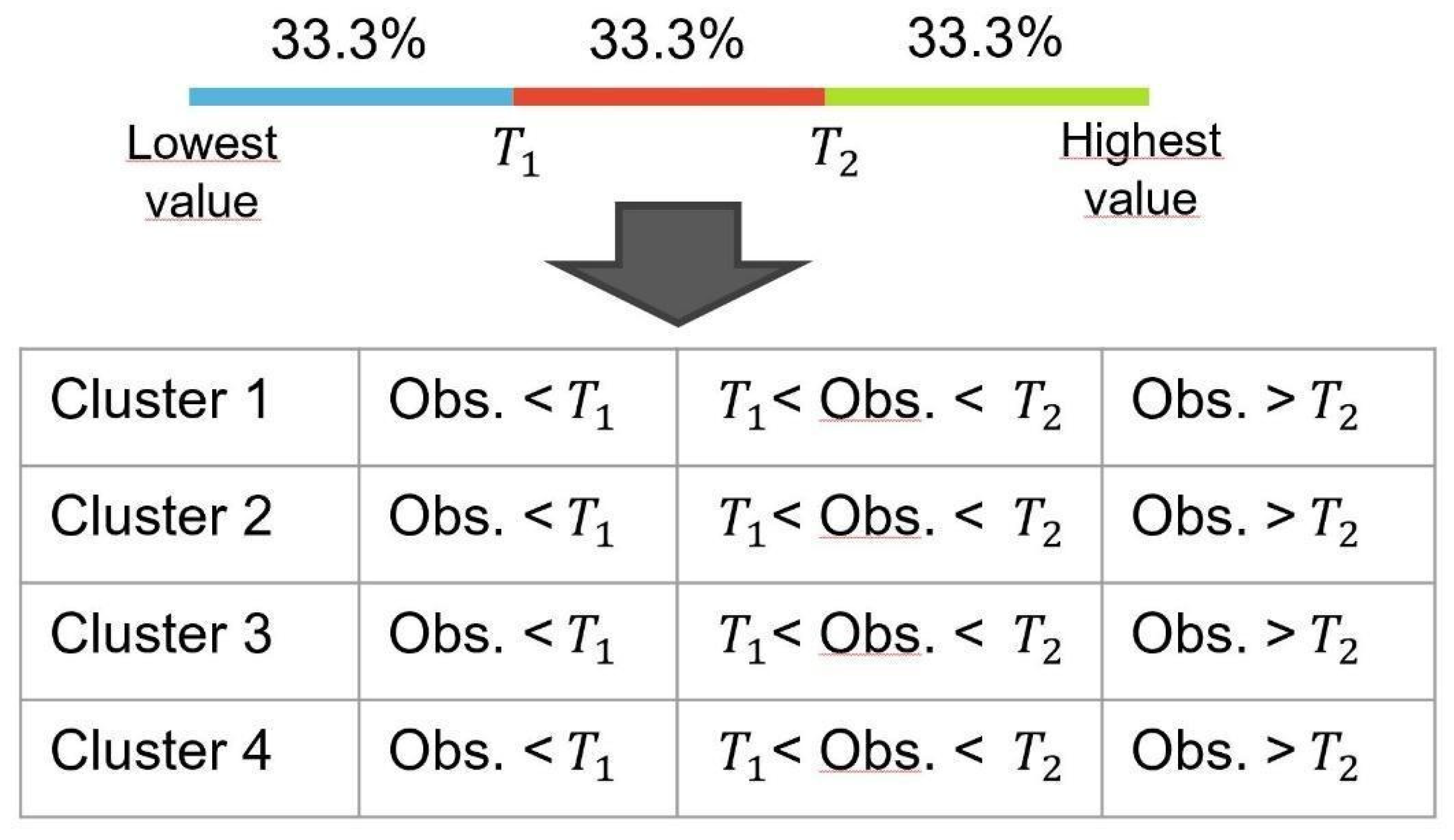
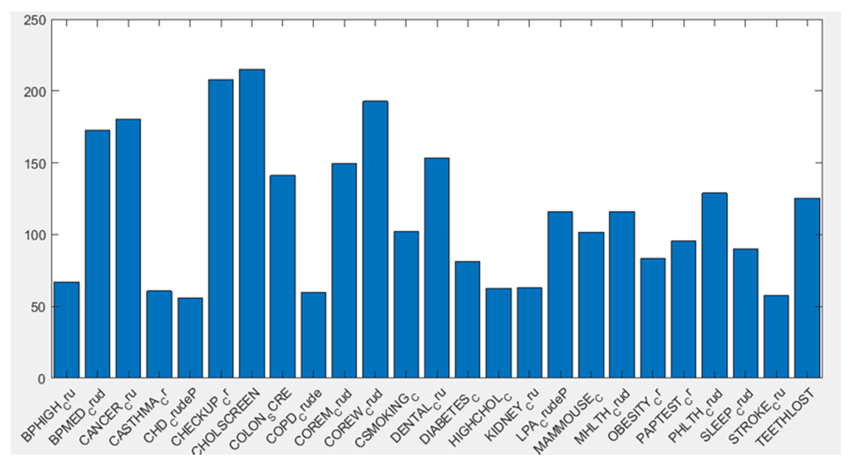
2.6. Correlation and Statistical Analysis
3. Results
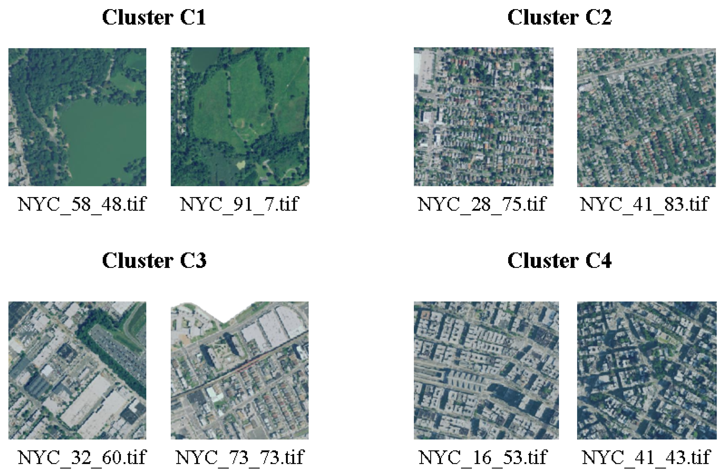
3.1. Clustering
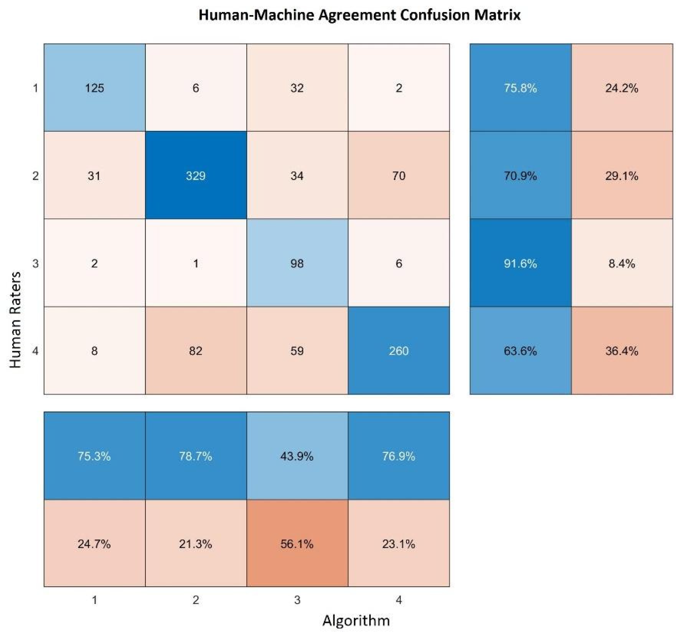
3.2. Clusters Validation with Inter-Rater Agreement and Cohen’s Kappa Coefficient
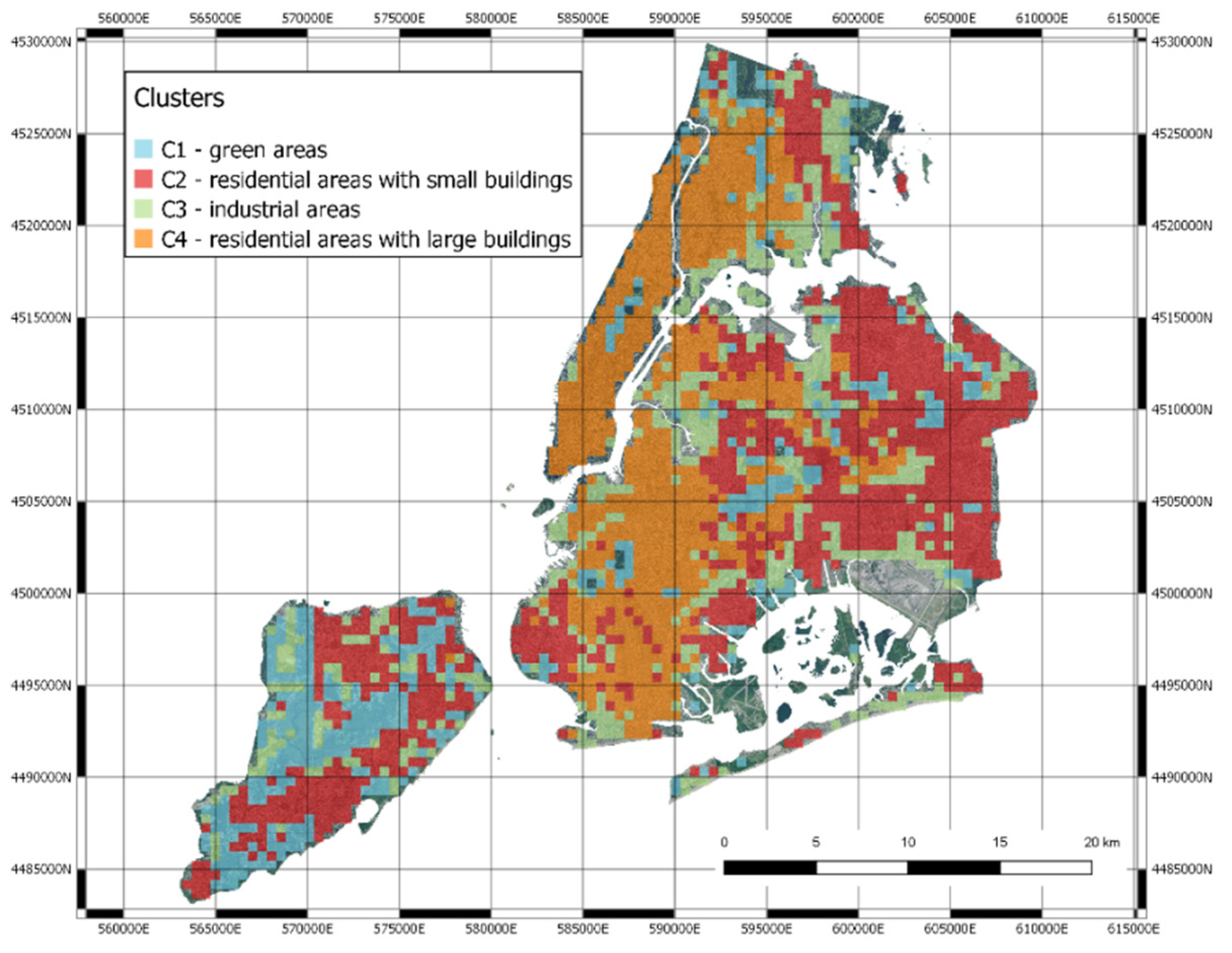
- Green areas (parks, gardens, nature);
- Residential areas with small houses;
- Industrial areas with factories, storage buildings and construction sites;
- Highly urbanized areas with large buildings.
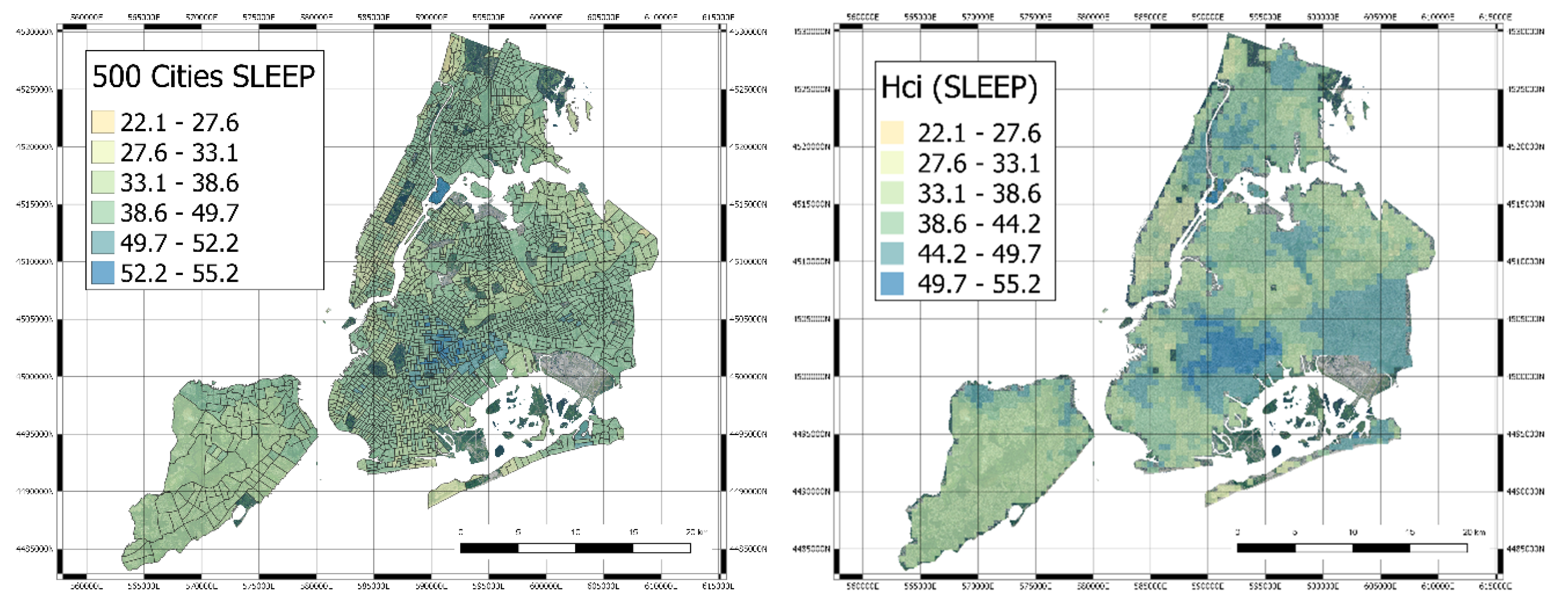
3.3. Mapping
4. Discussion
Author Contributions
Funding
Acknowledgments
Conflicts of Interest
References
- World Health Organization. UN-Habitat Global Report on Urban Health: Equitable Healthier Cities for Sustainable Development; World Health Organization: Geneva, Switzerland, 2016; ISBN 978-92-4-156527-1. [Google Scholar]
- Anandan, C.; Nurmatov, U.; van Schayck, O.C.P.; Sheikh, A. Is the prevalence of asthma declining? Systematic review of epidemiological studies. Allergy 2010, 65, 152–167. [Google Scholar] [CrossRef]
- Guarnieri, M.; Balmes, J.R. Outdoor air pollution and asthma. Lancet Lond. Engl. 2014, 383, 1581–1592. [Google Scholar] [CrossRef]
- Innovating Cities | Environment—Research and Innovation—European Commission. Available online: https://ec.europa.eu/research/environment/index.cfm?pg=future_cities (accessed on 13 November 2018).
- Kourou, K.; Exarchos, T.P.; Exarchos, K.P.; Karamouzis, M.V.; Fotiadis, D.I. Machine learning applications in cancer prognosis and prediction. Comput. Struct. Biotechnol. J. 2015, 13, 8–17. [Google Scholar] [CrossRef]
- Kuznietsov, Y.; Stuckler, J.; Leibe, B. Semi-Supervised Deep Learning for Monocular Depth Map Prediction. In Proceedings of the IEEE Conference on Computer Vision and Pattern Recognition (CVPR), Honolulu, HI, USA, 21–26 July 2017; pp. 6647–6655. [Google Scholar]
- George Karimpanal, T.; Bouffanais, R. Self-organizing maps for storage and transfer of knowledge in reinforcement learning. Adapt. Behav. 2019, 27, 111–126. [Google Scholar] [CrossRef]
- Bellazzi, R.; Caldarone, A.A.; Pala, D.; Franzini, M.; Malovini, A.; Larizza, C.; Casella, V. Transfer Learning for Urban Landscape Clustering and Correlation with Health Indexes. In Proceedings of the How AI Impacts Urban Living and Public Health; Pagán, J., Mokhtari, M., Aloulou, H., Abdulrazak, B., Cabrera, M.F., Eds.; Springer International Publishing: Cham, Switzerland, 2019; pp. 143–153. [Google Scholar]
- Krefis, A.C.; Augustin, M.; Schlünzen, K.H.; Oßenbrügge, J.; Augustin, J. How Does the Urban Environment Affect Health and Well-Being? A Systematic Review. Urban Sci. 2018, 2, 21. [Google Scholar] [CrossRef]
- Tavano Blessi, G.; Grossi, E.; Pieretti, G.; Ferilli, G.; Landi, A. Cities, the Urban Green Environment, and Individual Subjective Well-Being: The Case of Milan, Italy. Available online: https://www.hindawi.com/journals/usr/2015/137027/ (accessed on 29 February 2020).
- Helbich, M.; Yao, Y.; Liu, Y.; Zhang, J.; Liu, P.; Wang, R. Using deep learning to examine street view green and blue spaces and their associations with geriatric depression in Beijing, China. Environ. Int. 2019, 126, 107–117. [Google Scholar]
- Hong, K.Y.; Pinheiro, P.O.; Minet, L.; Hatzopoulou, M.; Weichenthal, S. Extending the spatial scale of land use regression models for ambient ultrafine particles using satellite images and deep convolutional neural networks. Environ. Res. 2019, 176, 108513. [Google Scholar] [CrossRef]
- Zewdie, G.K.; Lary, D.J.; Levetin, E.; Garuma, G.F. Applying Deep Neural Networks and Ensemble Machine Learning Methods to Forecast Airborne Ambrosia Pollen. Int. J. Environ. Res. Public Health 2019, 16, 1992. [Google Scholar] [CrossRef]
- Grekousis, G. Artificial neural networks and deep learning in urban geography: A systematic review and meta-analysis. Comput. Environ. Urban Syst. 2019, 74, 244–256. [Google Scholar] [CrossRef]
- Sharma, S.; Ball, J.E.; Tang, B.; Carruth, D.W.; Doude, M.; Islam, M.A. Semantic Segmentation with Transfer Learning for Off-Road Autonomous Driving. Sensors 2019, 19, 2577. [Google Scholar] [CrossRef]
- Team, K. Painter by Numbers Competition, 1st Place Winner’s Interview: Nejc Ilenič. 2019. Available online: https://medium.com/kaggle-blog/painter-by-numbers-competition-1st-place-winners-interview-nejc-ileni%C4%8D-4eaab5e6ce9d (accessed on 7 April 2020).
- 500 Cities Project: Local data for better health | Home page | CDC. Available online: https://www.cdc.gov/500cities/index.htm (accessed on 29 February 2020).
- Krieger, N. A Century of Census Tracts: Health & the Body Politic (1906–2006). J. Urban Health Bull. N. Y. Acad. Med. 2006, 83, 355–361. [Google Scholar]
- Domínguez-Berjón, M.F.; Borrell, C.; López, R.; Pastor, V. Mortality and socioeconomic deprivation in census tracts of an urban setting in Southern Europe. J. Urban Health Bull. N. Y. Acad. Med. 2005, 82, 225–236. [Google Scholar] [CrossRef][Green Version]
- Census Tract. Available online: https://factfinder.census.gov/help/en/census_tract.htm (accessed on 29 February 2020).
- Rao, J.N.K. Small-Area Estimation. In Wiley StatsRef: Statistics Reference Online; American Cancer Society: New York, NY, USA, 2017; pp. 1–8. ISBN 978-1-118-44511-2. [Google Scholar]
- Understanding World Files. Available online: http://webhelp.esri.com/arcims/9.3/General/topics/author_world_files.htm (accessed on 29 February 2020).
- Hu, Y.; Zhang, Q.; Zhang, Y.; Yan, H. A Deep Convolution Neural Network Method for Land Cover Mapping: A Case Study of Qinhuangdao, China. Remote Sens. 2018, 10, 2053. [Google Scholar] [CrossRef]
- Zhang, C.; Sargent, I.; Pan, X.; Li, H.; Gardiner, A.; Hare, J.; Atkinson, P.M. An object-based convolutional neural network (OCNN) for urban land use classification. Remote Sens. Environ. 2018, 216, 57–70. [Google Scholar] [CrossRef]
- Xia, X.; Xu, C.; Nan, B. Inception-v3 for flower classification. In Proceedings of the 2017 2nd International Conference on Image, Vision and Computing (ICIVC), Chengdu, China, 2–4 June 2017; pp. 783–787. [Google Scholar]
- VGG16—Convolutional Network for Classification and Detection. Available online: https://neurohive.io/en/popular-networks/vgg16/ (accessed on 29 February 2020).
- Mateen, M.; Wen, J.; Song, S.; Huang, Z. Fundus Image Classification Using VGG-19 Architecture with PCA and SVD. Symmetry 2019, 11, 1. [Google Scholar] [CrossRef]
- Almagro Armenteros, J.J.; Sønderby, C.K.; Sønderby, S.K.; Nielsen, H.; Winther, O. DeepLoc: Prediction of protein subcellular localization using deep learning. Bioinforma. Oxf. Engl. 2017, 33, 3387–3395. [Google Scholar] [CrossRef]
- Besenyei, E. OpenFace—Free and open source face recognition with deep neural networks—E&B Software. Available online: https://www.eandbsoftware.org/openface-free-and-open-source-face-recognition-with-deep-neural-networks/ (accessed on 7 April 2020).
- Arora, S.; Hu, W.; Kothari, P.K. An Analysis of the t-SNE Algorithm for Data Visualization. arXiv 2018, arXiv:180301768. [Google Scholar]
- Engstrom, L.; Tran, B.; Tsipras, D.; Schmidt, L.; Madry, A. Exploring the Landscape of Spatial Robustness. In Proceedings of the International Conference on Machine Learning, Long Beach, CA, USA, 10–15 June 2019; pp. 1802–1811. [Google Scholar]
- McHugh, M.L. Interrater reliability: The kappa statistic. Biochem. Med. 2012, 22, 276–282. [Google Scholar] [CrossRef]
- Clark, L.P.; Millet, D.B.; Marshall, J.D. Changes in Transportation-Related Air Pollution Exposures by Race-Ethnicity and Socioeconomic Status: Outdoor Nitrogen Dioxide in the United States in 2000 and 2010. Environ. Health Perspect. 2017, 125, 097012. [Google Scholar] [CrossRef]
- Litonjua, A.A.; Carey, V.J.; Weiss, S.T.; Gold, D.R. Race, socioeconomic factors, and area of residence are associated with asthma prevalence. Pediatr. Pulmonol. 1999, 28, 394–401. [Google Scholar] [CrossRef]
- Frontiers | Spatial Enablement to Support Environmental, Demographic, Socioeconomics, and Health Data Integration and Analysis for Big Cities: A Case Study with Asthma Hospitalizations in New York City | Medicine. Available online: https://www.frontiersin.org/articles/10.3389/fmed.2019.00084/full (accessed on 14 January 2020).
- Patel, C.J. Analytic Complexity and Challenges in Identifying Mixtures of Exposures Associated with Phenotypes in the Exposome Era. Curr. Epidemiol. Rep. 2017, 4, 22–30. [Google Scholar] [CrossRef]
- Kloog, I.; Ridgway, B.; Koutrakis, P.; Coull, B.A.; Schwartz, J.D. Long- and Short-Term Exposure to PM2.5 and Mortality. Epidemiol. Camb. Mass 2013, 24, 555–561. [Google Scholar] [CrossRef]


| Category | Measure |
|---|---|
| Health outcomes | Current asthma among adults aged >= 18 years High blood pressure among adults aged >= 18 years Cancer among adults aged ≥ 18 years High cholesterol among adults aged >= 18 years who have been screened in the past 5 years Chronic kidney disease among adults aged ≥ 18 years Chronic obstructive pulmonary disease among adults aged >= 18 years Coronary heart disease among adults aged ≥ 18 years Diagnosed diabetes among adults aged >= 18 years Mental health not good for >= 14 days among adults aged >= 18 years Physical health not good for >= 14 days among adults aged >= 18 years All teeth lost among adults aged >= 65 years Stroke among adults aged >= 18 years |
| Prevention | Visits to doctor for routine checkup within the past year among adults aged ≥ 18 years Visits to dentist or dental clinic among adults aged ≥ 18 years Taking medicine for high blood pressure control among adults aged ≥ 18 years with high blood pressure Cholesterol screening among adults aged ≥ 18 years Mammography use among women aged 50−74 years Papanicolaou smear use among adult women aged 21−65 years Fecal occult blood test, sigmoidoscopy, or colonoscopy among adults aged 50–75 years Older adults aged ≥ 65 years who are up to date on a core set of clinical preventive services by age and sex |
| Unhealthy behaviors | Current smoking among adults aged >= 18 years No leisure-time physical activity among adults aged >= 18 years Obesity among adults aged >= 18 years Sleeping less than 7 h among adults aged >= 18 years |
| Variable | C2 vs. C1 | C3 vs. C1 | C4 vs. C1 | |||
|---|---|---|---|---|---|---|
| OR (SE) | p | OR (SE) | p | OR (SE) | p | |
| ACCESS2_Cr | 1.07 (0.01) | <0.001 | 1.15 (0.01) | <0.001 | 1.17 (0.01) | <0.001 |
| BINGE_Crud | 0.81 (0.02) | <0.001 | 0.91 (0.02) | <0.001 | 1.01 (0.02) | 0.577 |
| BPHIGH_Cru | 1.06 (0.01) | <0.001 | 1.04 (0.01) | 0.004 | 0.98 (0.01) | 0.092 |
| BPMED_Crud | 1.09 (0.02) | <0.001 | 0.91 (0.02) | <0.001 | 0.87 (0.02) | <0.001 |
| CANCER_Cru | 0.86 (0.04) | <0.001 | 0.6 (0.05) | <0.001 | 0.47 (0.05) | <0.001 |
| CASTHMA_Cr | 1.35 (0.05) | <0.001 | 1.61 (0.05) | <0.001 | 1.77 (0.05) | <0.001 |
| CHD_CrudeP | 1.04 (0.04) | 0.374 | 0.98 (0.05) | 0.660 | 0.88 (0.05) | 0.005 |
| CHECKUP_Cr | 1.08 (0.02) | <0.001 | 0.94 (0.02) | 0.001 | 0.8 (0.02) | <0.001 |
| CHOLSCREEN | 0.95 (0.02) | 0.001 | 0.82 (0.02) | <0.001 | 0.74 (0.02) | <0.001 |
| COLON_SCRE | 0.97 (0.01) | 0.002 | 0.9 (0.01) | <0.001 | 0.88 (0.01) | <0.001 |
| COPD_Crude | 1.17 (0.04) | <0.001 | 1.25 (0.05) | <0.001 | 1.18 (0.04) | <0.001 |
| COREM_Crud | 0.88 (0.02) | <0.001 | 0.81 (0.02) | <0.001 | 0.77 (0.02) | <0.001 |
| COREW_Crud | 0.88 (0.01) | <0.001 | 0.82 (0.01) | <0.001 | 0.77 (0.01) | <0.001 |
| CSMOKING_C | 1.06 (0.02) | 0.001 | 1.18 (0.02) | <0.001 | 1.18 (0.02) | <0.001 |
| DENTAL_Cru | 0.94 (0.01) | <0.001 | 0.9 (0.01) | <0.001 | 0.9 (0.01) | <0.001 |
| DIABETES_C | 1.18 (0.02) | <0.001 | 1.25 (0.03) | <0.001 | 1.24 (0.02) | <0.001 |
| HIGHCHOL_C | 1.02 (0.02) | 0.306 | 0.92 (0.02) | <0.001 | 0.86 (0.02) | <0.001 |
| KIDNEY_Cru | 2.18 (0.14) | <0.001 | 2.82 (0.16) | <0.001 | 2.96 (0.15) | <0.001 |
| X.LPA_CrudeP | 1.09 (0.01) | <0.001 | 1.14 (0.01) | <0.001 | 1.14 (0.01) | <0.001 |
| MAMMOUSE_C | 0.98 (0.02) | 0.185 | 0.9 (0.02) | <0.001 | 0.83 (0.02) | <0.001 |
| MHLTH_Crud | 1.19 (0.03) | <0.001 | 1.41 (0.03) | <0.001 | 1.47 (0.03) | <0.001 |
| OBESITY_Cr | 1 (0.01) | 0.636 | 1.06 (0.01) | <0.001 | 1.02 (0.01) | 0.084 |
| PAPTEST_Cr | 0.85 (0.02) | <0.001 | 0.84 (0.02) | <0.001 | 0.81 (0.02) | <0.001 |
| PHLTH_Crud | 1.15 (0.02) | <0.001 | 1.28 (0.02) | <0.001 | 1.31 (0.02) | <0.001 |
| SLEEP_Crud | 1.15 (0.01) | <0.001 | 1.2 (0.02) | <0.001 | 1.19 (0.02) | <0.001 |
| STROKE_Cru | 1.51 (0.07) | <0.001 | 1.64 (0.08) | <0.001 | 1.61 (0.08) | <0.001 |
| TEETHLOST | 1.09 (0.01) | <0.001 | 1.15 (0.01) | <0.001 | 1.18 (0.01) | <0.001 |
| Variable | Interval | C2 vs. C1 | C3 vs. C1 | C4 vs. C1 | |||
|---|---|---|---|---|---|---|---|
| OR (SE) | p | OR (SE) | p | OR (SE) | p | ||
| ACCESS2_Cr | 12–18.95 | 2.6 (0.14) | <0.001 | 3.41 (0.17) | <0.001 | 2.93 (0.16) | <0.001 |
| ACCESS2_Cr | >=18.95 | 3.05 (0.18) | <0.001 | 10.48 (0.2) | <0.001 | 11.33 (0.19) | <0.001 |
| BINGE_Crud | 13.98–16.73 | 0.72 (0.16) | 0.045 | 1.05 (0.18) | 0.776 | 1.19 (0.17) | 0.306 |
| BINGE_Crud | >=16.73 | 0.25 (0.15) | <0.001 | 0.48 (0.17) | <0.001 | 0.73 (0.16) | 0.044 |
| BPHIGH_Cru | 28.4–32.9 | 3.65 (0.15) | <0.001 | 1.37 (0.17) | 0.064 | 0.92 (0.16) | 0.590 |
| BPHIGH_Cru | >=32.9 | 2.2 (0.15) | <0.001 | 1.43 (0.16) | 0.027 | 1.1 (0.15) | 0.530 |
| BPMED_Crud | 73.15–76.47 | 2.52 (0.17) | <0.001 | 0.69 (0.17) | 0.028 | 0.59 (0.15) | 0.001 |
| BPMED_Crud | >=76.47 | 2.84 (0.16) | <0.001 | 0.59 (0.17) | 0.001 | 0.21 (0.17) | <0.001 |
| CANCER_Cru | 4.7–5.95 | 1.71 (0.18) | 0.002 | 0.51 (0.18) | <0.001 | 0.36 (0.17) | <0.001 |
| CANCER_Cru | >=5.95 | 1.05 (0.16) | 0.769 | 0.24 (0.18) | <0.001 | 0.11 (0.17) | <0.001 |
| CASTHMA_Cr | 9.1–10.5 | 1.28 (0.14) | 0.073 | 1.53 (0.16) | 0.009 | 1.21 (0.15) | 0.204 |
| CASTHMA_Cr | >=10.5 | 2.48 (0.17) | <0.001 | 4.69 (0.19) | <0.001 | 5.23 (0.18) | <0.001 |
| CHD_CrudeP | 5.1–5.88 | 3.53 (0.15) | <0.001 | 1.28 (0.17) | 0.146 | 1.2 (0.16) | 0.257 |
| CHD_CrudeP | >=5.88 | 2.17 (0.15) | <0.001 | 1.27 (0.16) | 0.142 | 1.57 (0.15) | 0.003 |
| CHECKUP_Cr | 73.56–76.29 | 1.07 (0.17) | 0.686 | 0.32 (0.18) | <0.001 | 0.16 (0.16) | <0.001 |
| CHECKUP_Cr | >=76.29 | 2.05 (0.18) | <0.001 | 0.53 (0.18) | <0.001 | 0.19 (0.18) | <0.001 |
| CHOLSCREEN | 76.05–80.24 | 0.75 (0.19) | 0.125 | 0.3 (0.2) | <0.001 | 0.19 (0.18) | <0.001 |
| CHOLSCREEN | >=80.24 | 0.67 (0.18) | 0.028 | 0.17 (0.19) | <0.001 | 0.05 (0.2) | <0.001 |
| COLON_SCRE | 60.09–66.4 | 0.45 (0.19) | <0.001 | 0.23 (0.2) | <0.001 | 0.11 (0.19) | <0.001 |
| COLON_SCRE | >=66.4 | 0.56 (0.19) | 0.002 | 0.18 (0.2) | <0.001 | 0.12 (0.19) | <0.001 |
| COPD_Crude | 5.47–6.41 | 1.82 (0.14) | <0.001 | 1.44 (0.16) | 0.025 | 0.67 (0.16) | 0.010 |
| COPD_Crude | >=6.41 | 1.74 (0.16) | <0.001 | 2.07 (0.17) | <0.001 | 2.28 (0.16) | <0.001 |
| COREM_Crud | 25.43–31.74 | 0.61 (0.21) | 0.022 | 0.44 (0.22) | <0.001 | 0.25 (0.21) | <0.001 |
| COREM_Crud | >=31.74 | 0.27 (0.2) | <0.001 | 0.1 (0.22) | <0.001 | 0.06 (0.2) | <0.001 |
| COREW_Crud | 24.12–29.59 | 0.88 (0.21) | 0.552 | 0.4 (0.22) | <0.001 | 0.25 (0.21) | <0.001 |
| COREW_Crud | >=29.59 | 0.27 (0.19) | <0.001 | 0.11 (0.2) | <0.001 | 0.06 (0.2) | <0.001 |
| CSMOKING_C | 15.1–17.96 | 1.07 (0.13) | 0.596 | 1.84 (0.17) | <0.001 | 0.76 (0.15) | 0.078 |
| CSMOKING_C | >=17.96 | 1.83 (0.17) | 0.001 | 5.3 (0.19) | <0.001 | 4.97 (0.18) | <0.001 |
| DENTAL_Cru | 58.83–69.13 | 0.81 (0.2) | 0.288 | 0.39 (0.21) | <0.001 | 0.27 (0.2) | <0.001 |
| DENTAL_Cru | >=69.13 | 0.26 (0.18) | <0.001 | 0.1 (0.2) | <0.001 | 0.09 (0.19) | <0.001 |
| DIABETES_C | 9.11–11.64 | 2.3 (0.14) | <0.001 | 2.52 (0.16) | <0.001 | 1.36 (0.15) | 0.050 |
| DIABETES_C | >=11.64 | 3.09 (0.17) | <0.001 | 4.65 (0.19) | <0.001 | 5.2 (0.17) | <0.001 |
| HIGHCHOL_C | 36.22–39.25 | 2.16 (0.16) | <0.001 | 0.9 (0.17) | 0.556 | 0.71 (0.16) | 0.032 |
| HIGHCHOL_C | >=39.25 | 1.59 (0.15) | 0.002 | 0.62 (0.17) | 0.004 | 0.43 (0.15) | <0.001 |
| KIDNEY_Cru | 1.95–2.35 | 2.97 (0.15) | <0.001 | 2.28 (0.17) | <0.001 | 1.72 (0.16) | 0.001 |
| KIDNEY_Cru | >=2.35 | 1.83 (0.15) | <0.001 | 2.43 (0.17) | <0.001 | 3.06 (0.15) | <0.001 |
| X.LPA_CrudeP | 23.99–30.5 | 2.93 (0.14) | <0.001 | 2.5 (0.17) | <0.001 | 2.14 (0.16) | <0.001 |
| X.LPA_CrudeP | >=30.5 | 3.41 (0.18) | <0.001 | 7.28 (0.19) | <0.001 | 7.36 (0.18) | <0.001 |
| MAMMOUSE_C | 74.24–76.74 | 0.73 (0.17) | 0.055 | 0.47 (0.18) | <0.001 | 0.18 (0.17) | <0.001 |
| MAMMOUSE_C | >=76.74 | 0.99 (0.17) | 0.929 | 0.49 (0.18) | <0.001 | 0.26 (0.17) | <0.001 |
| MHLTH_Crud | 10.8–13.01 | 1.49 (0.13) | 0.003 | 2.81 (0.17) | <0.001 | 1.45 (0.15) | 0.017 |
| MHLTH_Crud | >=13.01 | 2.23 (0.18) | <0.001 | 7.3 (0.2) | <0.001 | 7.23 (0.18) | <0.001 |
| OBESITY_Cr | 23.17–28.85 | 0.53 (0.14) | <0.001 | 0.69 (0.17) | 0.034 | 0.24 (0.16) | <0.001 |
| OBESITY_Cr | >=28.85 | 1.26 (0.18) | 0.184 | 2.83 (0.19) | <0.001 | 1.44 (0.18) | 0.037 |
| PAPTEST_Cr | 79.76–84.2 | 0.44 (0.2) | <0.001 | 0.35 (0.21) | <0.001 | 0.2 (0.2) | <0.001 |
| PAPTEST_Cr | >=84.2 | 0.2 (0.19) | <0.001 | 0.18 (0.2) | <0.001 | 0.1 (0.19) | <0.001 |
| PHLTH_Crud | 10.68–13.24 | 2 (0.14) | <0.001 | 2.07 (0.17) | <0.001 | 1.39 (0.16) | 0.035 |
| PHLTH_Crud | >=13.24 | 2.65 (0.18) | <0.001 | 6.8 (0.19) | <0.001 | 7.83 (0.18) | <0.001 |
| SLEEP_Crud | 37.6–42.92 | 1.56 (0.14) | 0.001 | 4.11 (0.17) | <0.001 | 2.24 (0.15) | <0.001 |
| SLEEP_Crud | >=42.92 | 3.96 (0.18) | <0.001 | 9.75 (0.21) | <0.001 | 7.59 (0.19) | <0.001 |
| STROKE_Cru | 2.49–3.2 | 3.13 (0.15) | <0.001 | 1.9 (0.17) | <0.001 | 1.66 (0.16) | 0.001 |
| STROKE_Cru | >=3.2 | 2.1 (0.15) | <0.001 | 2.22 (0.17) | <0.001 | 2.87 (0.15) | <0.001 |
| TEETHLOST | 12.59–17.3 | 1.49 (0.13) | 0.003 | 2.09 (0.16) | <0.001 | 1 (0.16) | 0.982 |
| TEETHLOST | >=17.3 | 2.81 (0.19) | <0.001 | 6.38 (0.2) | <0.001 | 8.2 (0.19) | <0.001 |
| Variable | C2 vs. C1 | C3 vs. C1 | C4 vs. C1 | |||
|---|---|---|---|---|---|---|
| OR (SE) | p | OR (SE) | p | OR (SE) | p | |
| BPMED_Crud | 1.08 (0.12) | 0.524 | 0.65 (0.11) | <0.001 | 0.81 (0.11) | 0.046 |
| CANCER_Cru | 0.29 (0.4) | 0.002 | 0.83 (0.41) | 0.658 | 0.84 (0.4) | 0.664 |
| CASTHMA_Cr | 0.3 (0.48) | 0.012 | 0.58 (0.46) | 0.232 | 7.3 (0.46) | <0.001 |
| CHD_CrudeP | 15.53 (0.61) | <0.001 | 1.18 (0.63) | 0.788 | 1.21 (0.63) | 0.764 |
| CHECKUP_Cr | 0.73 (0.19) | 0.095 | 0.72 (0.19) | 0.083 | 0.38 (0.17) | <0.001 |
| COLON_SCRE | 1.89 (0.1) | <0.001 | 1.89 (0.1) | <0.001 | 2.1 (0.12) | <0.001 |
| COPD_Crude | 0.12 (0.53) | <0.001 | 0.21 (0.5) | 0.002 | 0.02 (0.53) | <0.001 |
| COREM_Crud | 0.93 (0.12) | 0.582 | 1.34 (0.13) | 0.026 | 1.08 (0.14) | 0.574 |
| COREW_Crud | 1.1 (0.11) | 0.414 | 0.74 (0.12) | 0.012 | 0.54 (0.13) | <0.001 |
| CSMOKING_C | 0.42 (0.24) | <0.001 | 0.91 (0.22) | 0.662 | 0.7 (0.23) | 0.124 |
| HIGHCHOL_C | 2.8 (0.17) | <0.001 | 2.2 (0.19) | <0.001 | 3.24 (0.2) | <0.001 |
| KIDNEY_Cru | 0 (0.76) | <0.001 | 0.09 (0.75) | 0.001 | 0 (0.77) | <0.001 |
| X.LPA_CrudeP | 1.2 (0.12) | 0.116 | 1.37 (0.11) | 0.006 | 0.99 (0.11) | 0.925 |
| MAMMOUSE_C | 0.91 (0.11) | 0.396 | 0.65 (0.11) | <0.001 | 0.57 (0.11) | <0.001 |
| MHLTH_Crud | 95.21 (0.52) | <0.001 | 5.03 (0.48) | 0.001 | 1.94 (0.51) | 0.195 |
| OBESITY_Cr | 0.87 (0.05) | 0.004 | 1.01 (0.05) | 0.854 | 0.81 (0.05) | <0.001 |
| PHLTH_Crud | 0.08 (0.52) | <0.001 | 0.29 (0.47) | 0.008 | 0.62 (0.48) | 0.324 |
| SLEEP_Crud | 1.59 (0.16) | 0.004 | 1.43 (0.17) | 0.031 | 1.32 (0.16) | 0.079 |
| STROKE_Cru | 6.86 (0.59) | 0.001 | 42.51 (0.57) | <0.001 | 384.21 (0.61) | <0.001 |
| TEETHLOST | 1.93 (0.15) | <0.001 | 1.13 (0.15) | 0.428 | 1.56 (0.15) | 0.004 |
| Variable | C2 vs. C1 | C3 vs. C1 | C4 vs. C1 | |||
|---|---|---|---|---|---|---|
| OR (SE) | p | OR (SE) | p | OR (SE) | p | |
| BPHIGH_Cru2 | 1.02 (0.29) | 0.947 | 1.31 (0.33) | 0.422 | 1.17 (0.34) | 0.635 |
| BPHIGH_Cru3 | 0.24 (0.45) | 0.001 | 0.43 (0.51) | 0.100 | 0.45 (0.53) | 0.130 |
| BPMED_Crud2 | 0.97 (0.34) | 0.919 | 0.46 (0.36) | 0.032 | 0.55 (0.35) | 0.086 |
| BPMED_Crud3 | 1.9 (0.46) | 0.165 | 0.59 (0.5) | 0.293 | 0.48 (0.5) | 0.144 |
| CANCER_Cru2 | 1.43 (0.34) | 0.294 | 0.94 (0.35) | 0.855 | 0.86 (0.34) | 0.670 |
| CANCER_Cru3 | 0.65 (0.48) | 0.370 | 0.74 (0.52) | 0.569 | 0.61 (0.5) | 0.318 |
| CASTHMA_Cr2 | 1.2 (0.24) | 0.432 | 0.82 (0.28) | 0.483 | 1.15 (0.3) | 0.628 |
| CASTHMA_Cr3 | 1.4 (0.49) | 0.490 | 1.45 (0.52) | 0.480 | 6.17 (0.55) | 0.001 |
| CHD_CrudeP2 | 2.69 (0.25) | <0.001 | 2.08 (0.29) | 0.011 | 3.54 (0.3) | <0.001 |
| CHD_CrudeP3 | 3.13 (0.38) | 0.003 | 5.07 (0.43) | <0.001 | 15.13 (0.44) | <0.001 |
| CHECKUP_Cr2 | 1.32 (0.32) | 0.392 | 0.79 (0.34) | 0.471 | 0.42 (0.33) | 0.009 |
| CHECKUP_Cr3 | 2.61 (0.43) | 0.025 | 1.15 (0.47) | 0.767 | 0.24 (0.47) | 0.002 |
| CHOLSCREEN2 | 0.71 (0.34) | 0.320 | 0.54 (0.36) | 0.088 | 0.77 (0.35) | 0.450 |
| CHOLSCREEN3 | 0.44 (0.45) | 0.066 | 0.31 (0.49) | 0.016 | 0.24 (0.48) | 0.003 |
| COLON_SCRE2 | 1.59 (0.36) | 0.200 | 1.75 (0.38) | 0.138 | 0.77 (0.38) | 0.489 |
| COLON_SCRE3 | 7.47 (0.44) | <0.001 | 5.42 (0.49) | 0.001 | 2.04 (0.5) | 0.153 |
| COPD_Crude2 | 2.36 (0.25) | 0.001 | 1.99 (0.29) | 0.016 | 0.98 (0.3) | 0.954 |
| COPD_Crude3 | 2.85 (0.36) | 0.004 | 2.16 (0.41) | 0.061 | 1.16 (0.42) | 0.730 |
| COREM_Crud2 | 0.84 (0.38) | 0.640 | 0.87 (0.39) | 0.728 | 0.32 (0.41) | 0.005 |
| COREM_Crud3 | 0.68 (0.53) | 0.463 | 0.57 (0.58) | 0.330 | 0.3 (0.59) | 0.040 |
| COREW_Crud2 | 0.66 (0.4) | 0.308 | 0.58 (0.42) | 0.193 | 0.23 (0.43) | 0.001 |
| COREW_Crud3 | 0.66 (0.55) | 0.453 | 0.81 (0.61) | 0.734 | 0.15 (0.6) | 0.002 |
| DENTAL_Cru2 | 1.15 (0.42) | 0.733 | 0.79 (0.44) | 0.595 | 1.73 (0.45) | 0.219 |
| DENTAL_Cru3 | 0.56 (0.54) | 0.292 | 0.3 (0.59) | 0.044 | 0.6 (0.62) | 0.407 |
| HIGHCHOL_C2 | 0.96 (0.28) | 0.876 | 0.77 (0.29) | 0.371 | 0.41 (0.29) | 0.003 |
| HIGHCHOL_C3 | 0.52 (0.41) | 0.112 | 0.59 (0.44) | 0.221 | 0.23 (0.44) | 0.001 |
| KIDNEY_Cru2 | 0.95 (0.24) | 0.843 | 0.87 (0.28) | 0.635 | 1.14 (0.29) | 0.657 |
| KIDNEY_Cru3 | 0.37 (0.42) | 0.017 | 0.49 (0.47) | 0.135 | 1.77 (0.48) | 0.233 |
| X.LPA_CrudeP2 | 1.12 (0.33) | 0.726 | 0.81 (0.38) | 0.593 | 1.26 (0.4) | 0.569 |
| X.LPA_CrudeP3 | 1.33 (0.5) | 0.571 | 1.11 (0.55) | 0.843 | 0.56 (0.57) | 0.305 |
| MHLTH_Crud2 | 1.16 (0.25) | 0.555 | 1.95 (0.31) | 0.034 | 1.24 (0.34) | 0.529 |
| MHLTH_Crud3 | 0.55 (0.47) | 0.212 | 0.76 (0.53) | 0.613 | 0.6 (0.57) | 0.372 |
| OBESITY_Cr2 | 0.45 (0.25) | 0.001 | 0.35 (0.29) | <0.001 | 0.07 (0.3) | <0.001 |
| OBESITY_Cr3 | 0.37 (0.45) | 0.024 | 0.39 (0.48) | 0.053 | 0.04 (0.5) | <0.001 |
| PAPTEST_Cr2 | 0.59 (0.31) | 0.083 | 0.86 (0.33) | 0.655 | 0.76 (0.33) | 0.408 |
| PAPTEST_Cr3 | 0.24 (0.4) | <0.001 | 0.65 (0.44) | 0.327 | 0.7 (0.45) | 0.428 |
| SLEEP_Crud2 | 1 (0.3) | 0.992 | 2.18 (0.35) | 0.026 | 0.38 (0.37) | 0.008 |
| SLEEP_Crud3 | 4.26 (0.5) | 0.004 | 4.45 (0.54) | 0.006 | 0.54 (0.55) | 0.260 |
© 2020 by the authors. Licensee MDPI, Basel, Switzerland. This article is an open access article distributed under the terms and conditions of the Creative Commons Attribution (CC BY) license (http://creativecommons.org/licenses/by/4.0/).
Share and Cite
Pala, D.; Caldarone, A.A.; Franzini, M.; Malovini, A.; Larizza, C.; Casella, V.; Bellazzi, R. Deep Learning to Unveil Correlations between Urban Landscape and Population Health. Sensors 2020, 20, 2105. https://doi.org/10.3390/s20072105
Pala D, Caldarone AA, Franzini M, Malovini A, Larizza C, Casella V, Bellazzi R. Deep Learning to Unveil Correlations between Urban Landscape and Population Health. Sensors. 2020; 20(7):2105. https://doi.org/10.3390/s20072105
Chicago/Turabian StylePala, Daniele, Alessandro Aldo Caldarone, Marica Franzini, Alberto Malovini, Cristiana Larizza, Vittorio Casella, and Riccardo Bellazzi. 2020. "Deep Learning to Unveil Correlations between Urban Landscape and Population Health" Sensors 20, no. 7: 2105. https://doi.org/10.3390/s20072105
APA StylePala, D., Caldarone, A. A., Franzini, M., Malovini, A., Larizza, C., Casella, V., & Bellazzi, R. (2020). Deep Learning to Unveil Correlations between Urban Landscape and Population Health. Sensors, 20(7), 2105. https://doi.org/10.3390/s20072105