Automatic Seamline Determination for Urban Image Mosaicking Based on Road Probability Map from the D-LinkNet Neural Network


Abstract
:1. Introduction
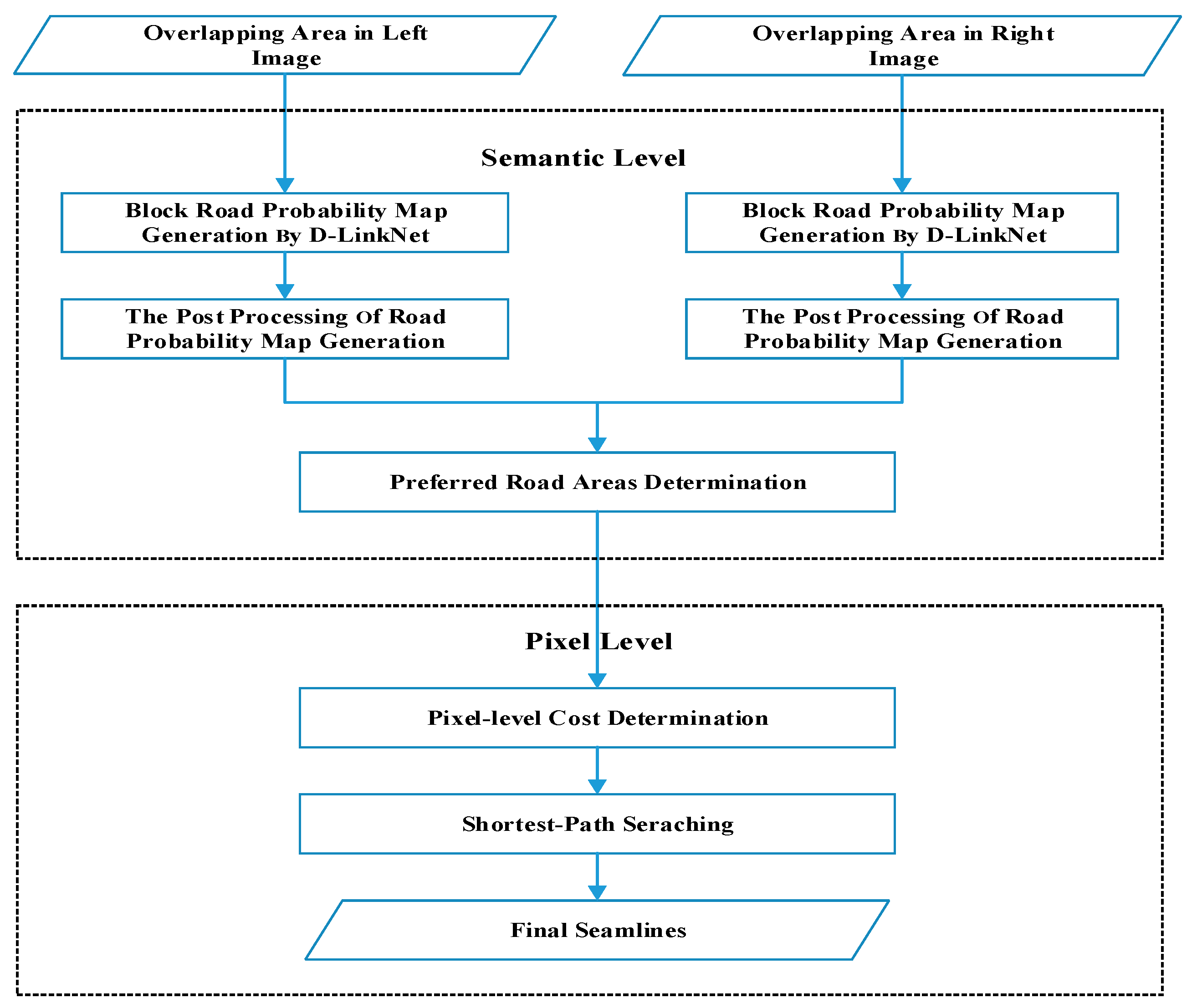
2. Materials and Methods
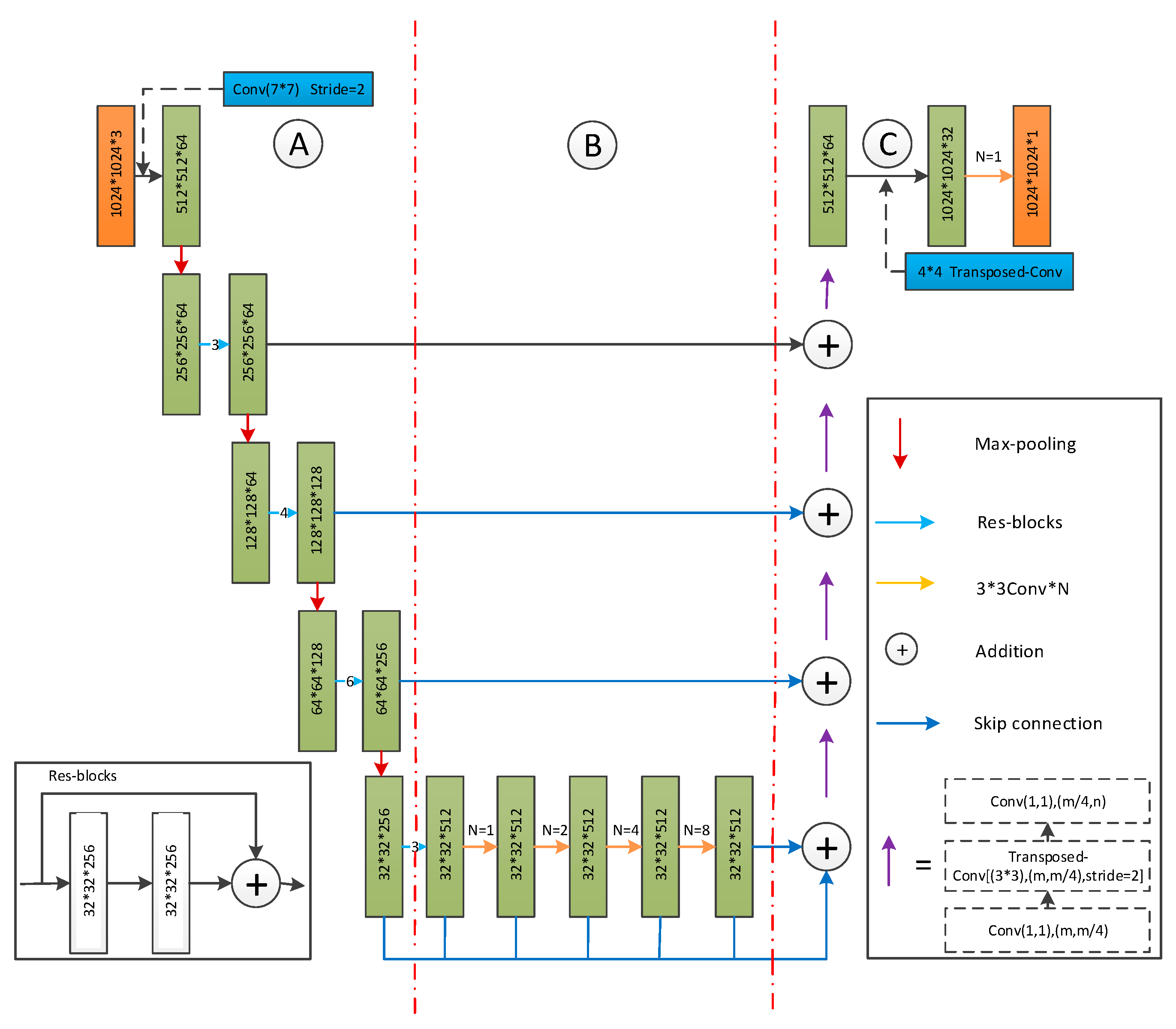
2.1. Road Probability Map Generation by D-LinkNet
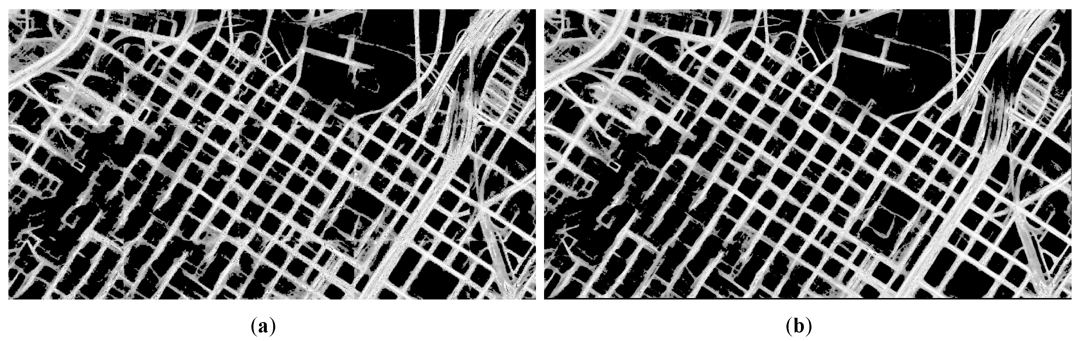
2.1.1. Block Road Probability Map Generation by D-Linknet
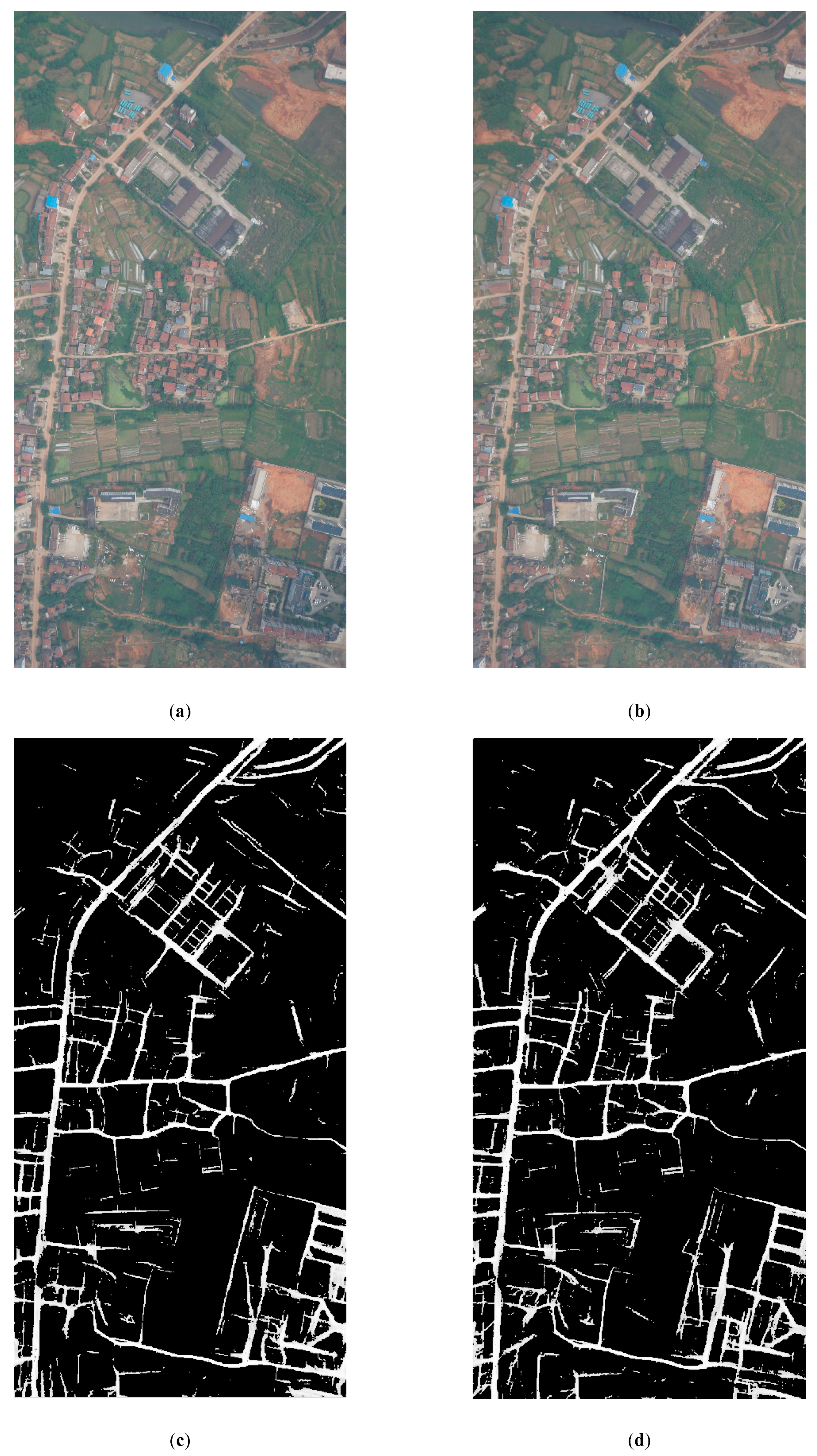
2.1.2. The Post Processing of Road Probability Map Generation
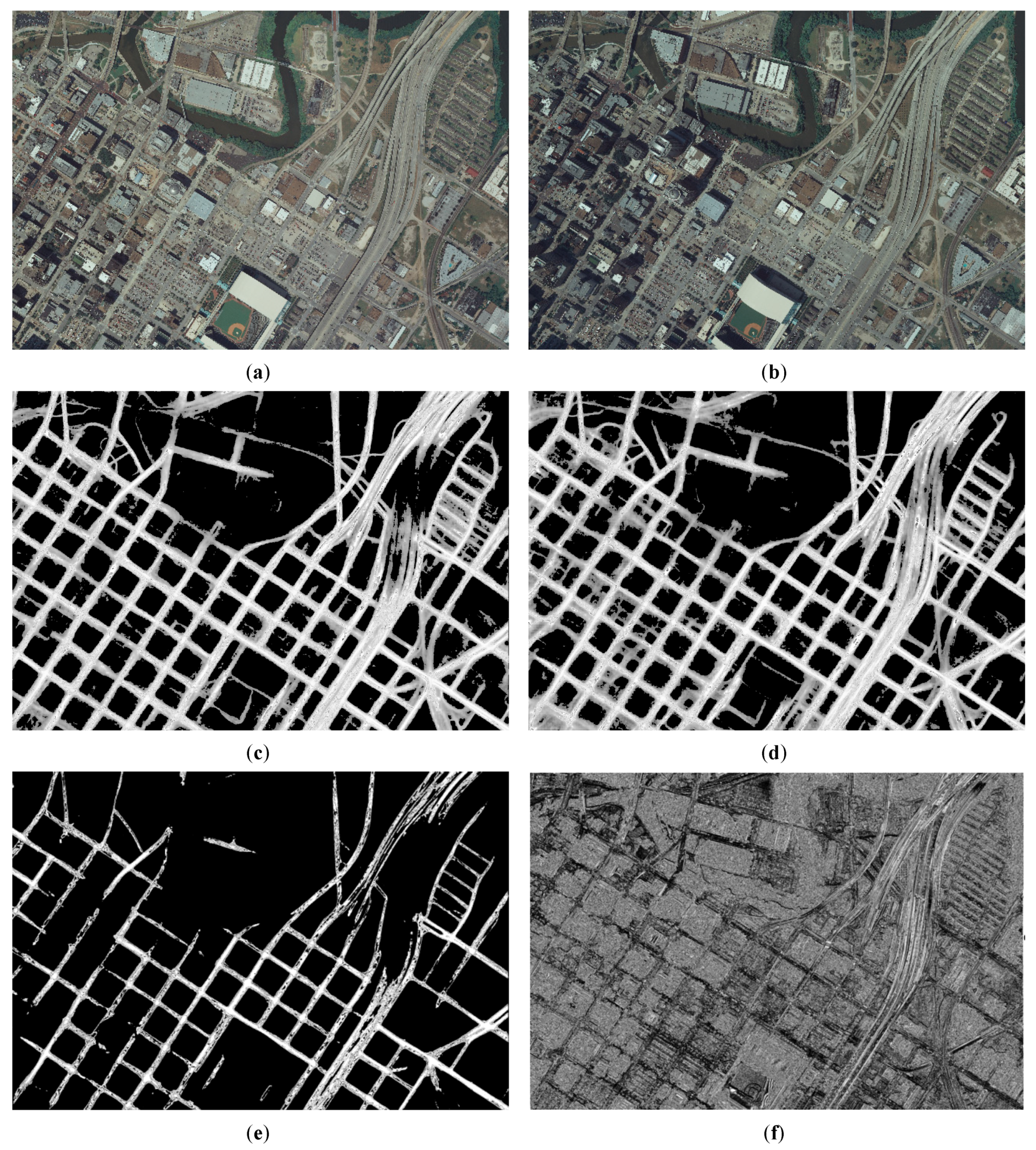
2.2. Preferred Road Areas Determination
2.3. Pixel-Level Seamline Determination
2.3.1. Pixel-Level Cost Determination
2.3.2. Shortest-Path Searching
| Algorithm 1 Dijkstra’s algorithm | |
| 1 | Dijkstra(G, s) |
| 2 | dist[s] = 0 |
| 3 | for each vertex v∈V |
| 4 | if v ≠ s |
| 5 | dist[v] = ∞ |
| 6 | pre [v] = undefined |
| 7 | S = Ø |
| 8 | Q = V |
| 9 | whileQ ≠ Ø do |
| 10 | u = extract_min(Q) |
| 11 | S = S∪{u} |
| 12 | for each vertex v∈Adj(u) do |
| 13 | dist[v] = min(dist[v], dist[u]+w(u, v)) |
| 14 | pre[v] = u |
| Algorithm 2 Dijkstra’s algorithm with Binary Min-heap | |
| 1 | Dijkstra_Binary_Min-heap(G, s) |
| 2 | dist[s] = 0 |
| 3 | for each vertex v∈V |
| 4 | if v ≠ s |
| 5 | dist[v] = ∞ |
| 6 | pre [v] = undefined |
| 7 | Q.add_with_min-priority(v, dist[v]) |
| 8 | S = Ø |
| 9 | Q = V |
| 10 | whileQ ≠ Ø do |
| 11 | u = extract_min_with_min- priority(Q) |
| 12 | S = S∪{u} |
| 13 | for each vertex v∈Adj(u) do |
| 14 | dist[v] = min(dist[v], dist[u]+w(u, v)) |
| 15 | pre[v] = u |
| 16 | Q.decrease_min-priority(v, dist[v]) |
3. Experimental Results and Analysis
3.1. Experimental Data and Platform
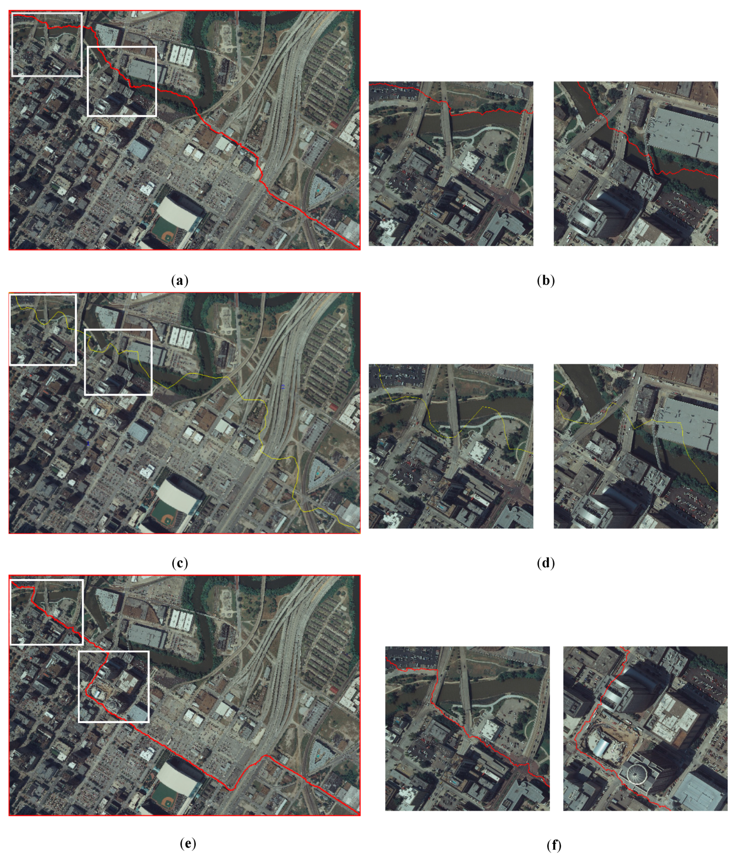
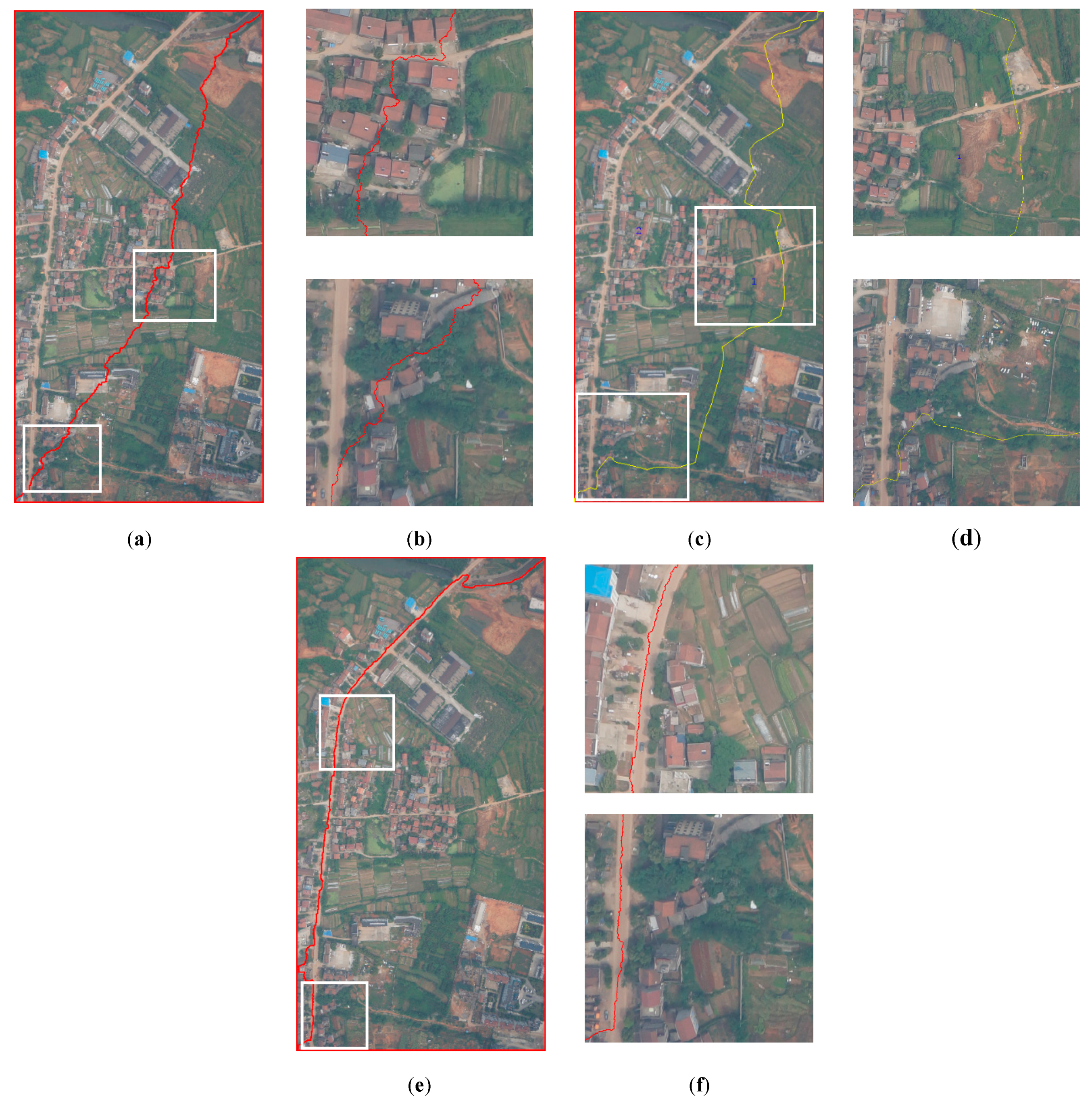
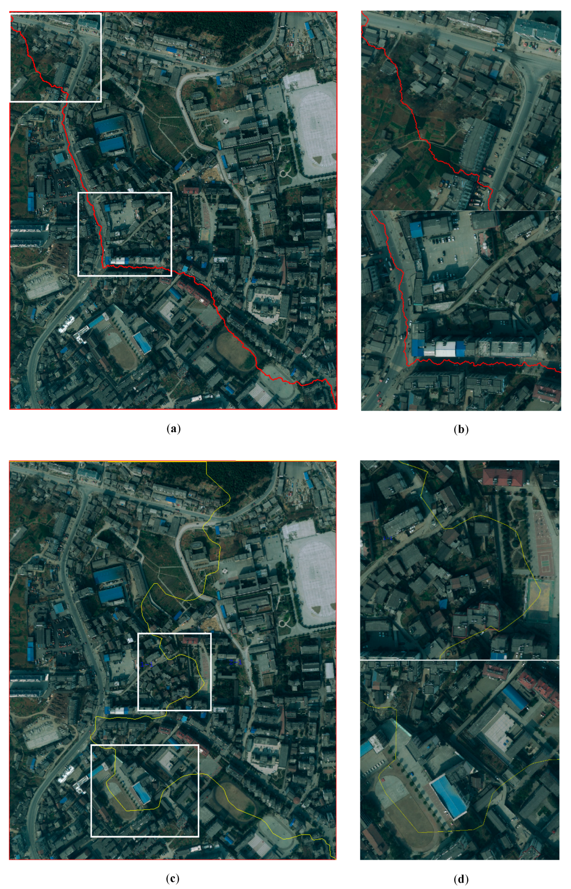
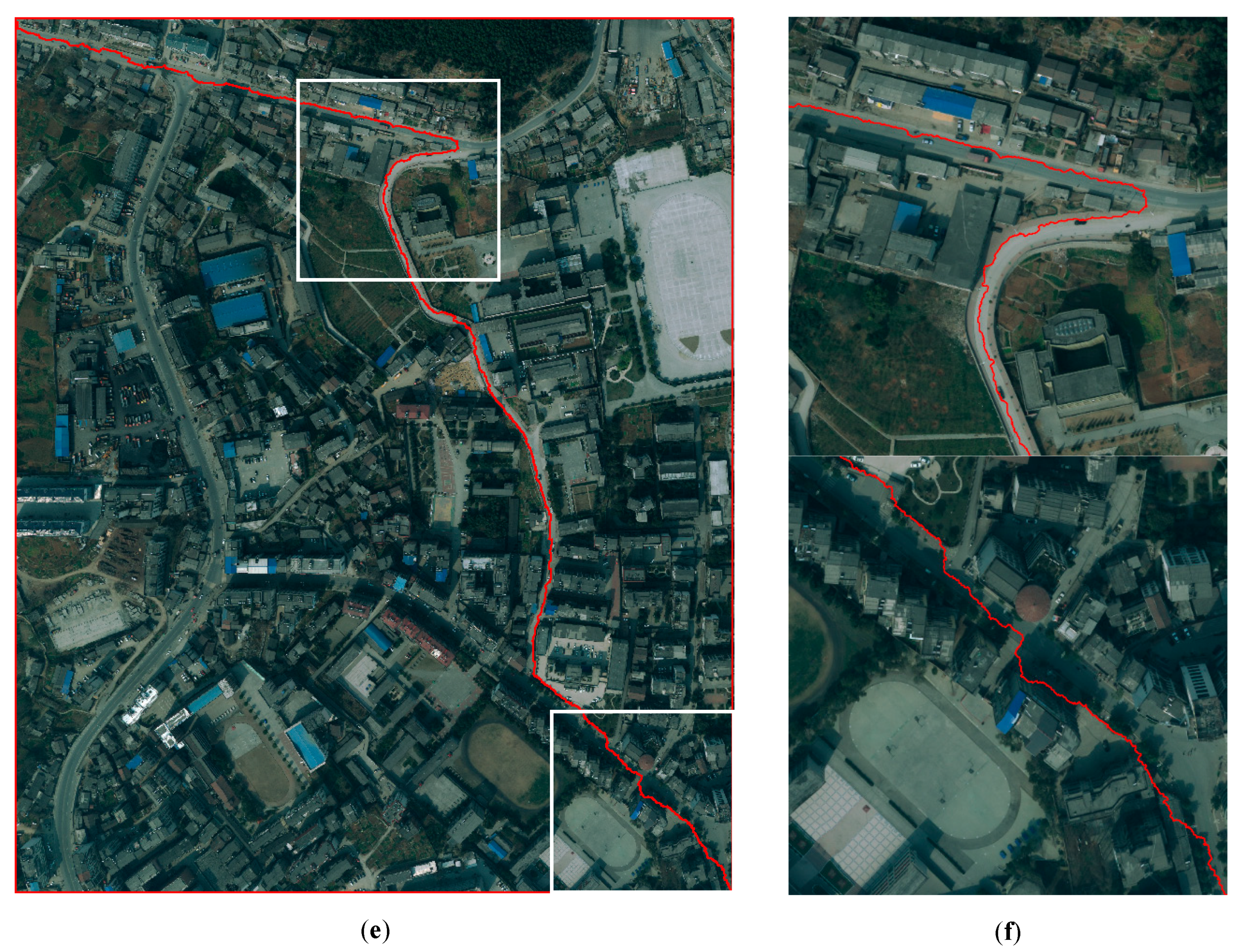
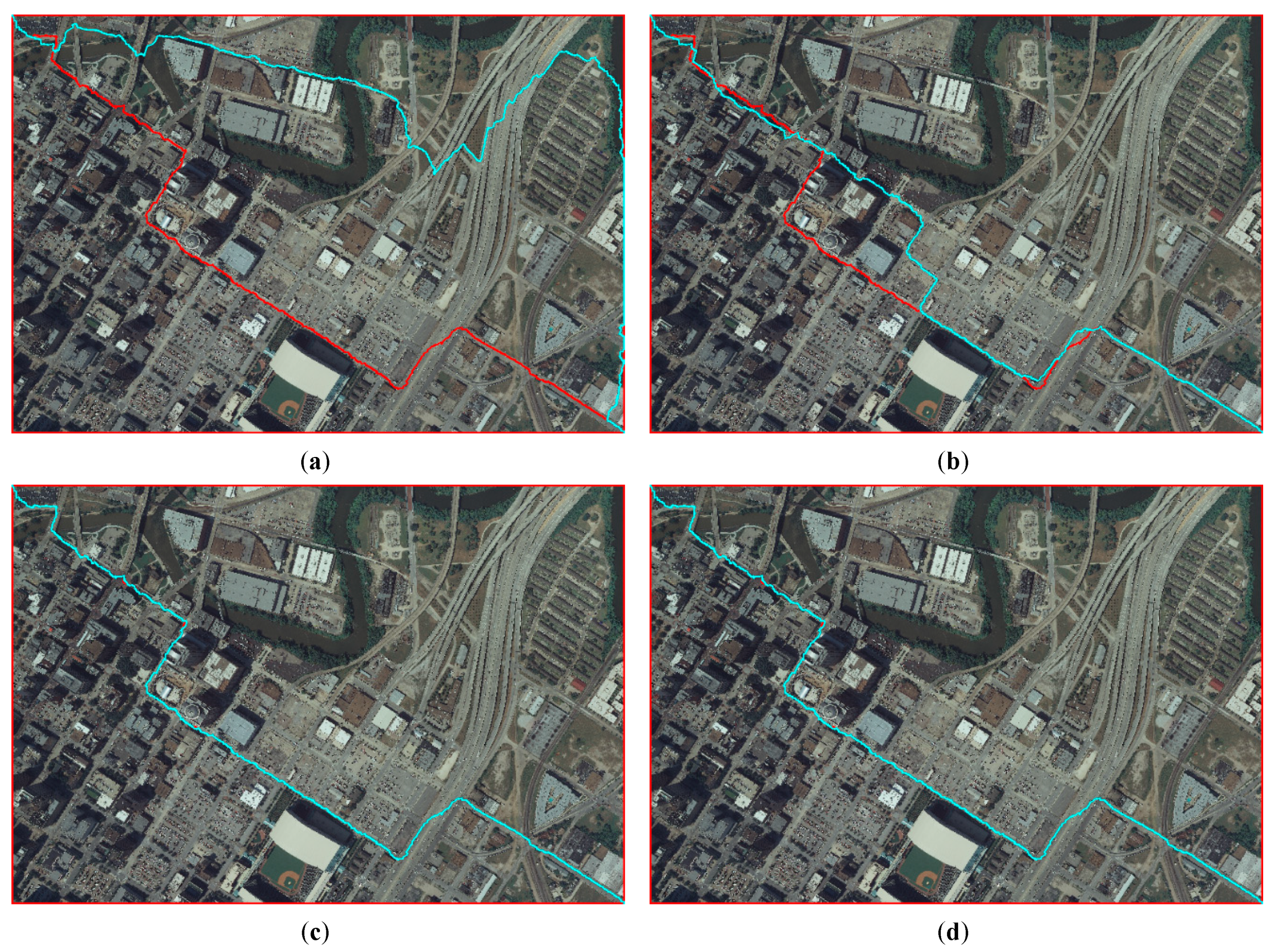
3.2. Seamline Determination Results and Analysis
4. Conclusions
Author Contributions
Funding
Conflicts of Interest
References
- Kerschner, M. Seamline detection in colour orthoimage mosaicking by use of twin snakes. ISPRS J. Photogramm. Remote Sens. 2001, 56, 53–64. [Google Scholar] [CrossRef]
- Wang, D.; Cao, W.; Xin, X.; Shao, P.; Brolly, M.; Xiao, J.; Wan, Y.; Zhang, Y. Using vector building maps to aid in generating seams for low-attitude aerial orthoimage mosaicking: Advantages in avoiding the crossing of buildings. ISPRS J. Photogramm. Remote Sens. 2017, 125, 207–224. [Google Scholar] [CrossRef]
- Pan, J.; Wang, M.; Ma, D.; Zhou, Q.; Li, J. Seamline network refinement based on area Voronoi diagrams 1with overlap. IEEE Trans. Geosci. Remote Sens. 2014, 52, 1658–1666. [Google Scholar] [CrossRef]
- He, J.; Sun, M.; Chen, Q.; Zhang, Z. An improved approach for generating globally consistent seamline networks for aerial image mosaicking. Int. J. Remote Sens. 2019, 40, 859–882. [Google Scholar] [CrossRef]
- Zheng, M.; Xiong, X.; Zhu, J. A novel orthoimage mosaic method using a weighted a* algorithm—Implementation and evaluation. ISPRS J. Photogramm. Remote Sens. 2018, 138, 30–46. [Google Scholar] [CrossRef]
- Pan, J.; Zhou, Q.; Wang, M. Seamline determination based on segmentation for urban image mosaicking. IEEE Trans. Geosci. Remote Sens. Lett. 2014, 11, 1335–1339. [Google Scholar] [CrossRef]
- Wang, M.; Yuan, S.; Pan, J.; Fang, L.; Zhou, Q.; Yang, G. Seamline determination for high resolution orthoimage mosaicking using watershed segmentation. Photogramm. Eng. Remote Sens. 2016, 82, 121–133. [Google Scholar] [CrossRef]
- Dong, Q.; Liu, J. Seamline Determination Based on PKGC Segmentation for Remote Sensing Image Mosaicking. Sensors 2017, 17, 1721. [Google Scholar] [CrossRef]
- Milgram, D.L. Computer methods for creating photomosaics. IEEE Trans. Comput. 1975, 24, 1113–1119. [Google Scholar] [CrossRef]
- Afek, Y.; Brand, A. Mosaicking of orthorectified aerial images. Photogramm. Eng. Remote Sens. 1998, 64, 115–124. [Google Scholar]
- Soille, P. Morphological image compositing. IEEE Trans. Pattern Anal. Mach. Intell. 2006, 28, 673–683. [Google Scholar] [CrossRef] [PubMed]
- Wang, L.; Ai, H.; Zhang, L. Automated seamline detection in orthophoto mosaicking using improved snakes. In Proceedings of the International Conference on Information Engineering and Computer Science (ICIECS), Wuhan, China, 25–26 December 2010; pp. 1–4. [Google Scholar]
- Ma, H.; Sun, J. Intelligent optimization of seam-line finding for orthophoto mosaicking with LiDAR point clouds. J. Zhejiang Univ. Sci. C 2011, 12, 417–429. [Google Scholar] [CrossRef]
- Wang, D.; Wan, Y.; Xiao, J.; Lai, X.; Huang, W.; Xu, J. Aerial image mosaicking with the aid of vector roads. Photogramm. Eng. Remote Sens. 2012, 78, 1141–1150. [Google Scholar] [CrossRef]
- Wan, Y.; Wang, D.; Xiao, J.; Wang, X.; Yu, Y.; Xu, J. Tracking of vector roads for the determination of seams in aerial image mosaics. IEEE Geosci. Remote Sens. Lett. 2012, 9, 328–332. [Google Scholar] [CrossRef]
- Wan, Y.; Wang, D.; Xiao, J.; Lai, X.; Xu, J. Automatic determination of seamlines for aerial image mosaicking based on vector roads alone. ISPRS J. Photogramm. Remote Sens. 2013, 76, 1–10. [Google Scholar] [CrossRef]
- Chen, Q.; Sun, M.; Hu, X.; Zhang, Z. Automatic seamline network generation for urban orthophoto mosaicking with the use of a digital surface Model. Remote Sens. 2014, 6, 12334–12359. [Google Scholar] [CrossRef] [Green Version]
- Pan, J.; Yuan, S.; Li, J.; Wu, B. Seamline optimization based on ground objects classes for orthoimage mosaicking. Remote Sens. Lett. 2017, 8, 280–289. [Google Scholar] [CrossRef]
- Chon, J.; Kim, H.; Lin, C.S. Seam-line determination for image mosaicking: A technique minimizing the maximum local mismatch and the global cost. ISPRS J. Photogramm. Remote Sens. 2010, 65, 86–92. [Google Scholar] [CrossRef]
- Pan, J.; Wang, M.; Li, J.; Yuan, S.; Hu, F. Region change rate-driven seamline determination method. ISPRS J. Photogramm. Remote Sens. 2015, 105, 141–154. [Google Scholar] [CrossRef]
- Li, L.; Yao, J.; Lu, X.; Tu, J.; Shan, J. Optimal seamline detection for multiple image mosaicking via graph cuts. ISPRS J. Photogramm. Remote Sens. 2016, 113, 1–16. [Google Scholar] [CrossRef]
- Li, L.; Yao, J.; Shi, S.; Yuan, S.; Zhang, Y.; Li, J. Superpixel-based optimal seamline detection in the gradient domain via graph cuts for orthoimage mosaicking. Int. J. Remote Sens. 2018, 39, 3908–3925. [Google Scholar] [CrossRef]
- Li, M.; Li, D.; Guo, B.; Li, L.; Wu, T.; Zhang, W. Automatic seam-line detection in UAV remote sensing image mosaicking by use of graph cuts. ISPRS Int. J. Geo-Inf. 2018, 9, 361. [Google Scholar] [CrossRef] [Green Version]
- Yuan, X.; Duan, M.; Cao, J. A seam line detection algorithm for orthophoto mosaicking based on disparity image. Acta Geod. Cartogr. Sin. 2015, 44, 877–883. [Google Scholar]
- Pang, S.; Sun, M.; Hu, X.; Zhang, Z. SGM-based seamline determination for urban orthophoto mosaicking. ISPRS J. Photogramm. Remote Sens. 2016, 112, 1–12. [Google Scholar] [CrossRef]
- Li, L.; Yao, J.; Liu, Y.; Yuan, W.; Shi, S.; Yuan, S. Optimal seamline detection for orthoimage mosaicking by combining deep convolutional neural network and graph cuts. Remote Sens. 2017, 9, 701. [Google Scholar] [CrossRef] [Green Version]
- Tupin, F.; Maitre, H.; Mangin, J.F.; Nicolas, J.M.; Pechersky, E. Detection of linear features in SAR images: Application to road network extraction. IEEE Trans. Geosci. Remote Sens. 1998, 36, 434–453. [Google Scholar] [CrossRef] [Green Version]
- Zhou, T.; Sun, C.; Fu, H. Road information extraction from high-resolution remote sensing images based on road reconstruction. Remote Sens. 2019, 11, 79. [Google Scholar] [CrossRef] [Green Version]
- Sun, L.; Tang, Y.; Zhang, L. Rural building detection in high-resolution imagery based on a two-stage cnn model. IEEE Geosci. Remote Sens. Lett. 2017, 14, 1998–2002. [Google Scholar] [CrossRef]
- Zhang, Z.; Liu, Q.; Wang, Y. Road extraction by deep residual U-Net. IEEE Geosci. Remote Sens. Lett. 2018, 15, 749–753. [Google Scholar] [CrossRef] [Green Version]
- Wei, Y.; Wang, Z.; Xu, M. Road structure refined CNN for road extraction in aerial image. IEEE Geosci. Remote Sens. Lett. 2017, 14, 709–713. [Google Scholar] [CrossRef]
- Lyu, Y.; Huang, X. Road segmentation using CNN with GRU. arXiv 2018, arXiv:1804.05164. [Google Scholar]
- Ma, J.; Zhao, J. Robust topological navigation via convolutional neural network feature and sharpness measure. IEEE Access 2017, 5, 20707–20715. [Google Scholar] [CrossRef]
- Zhou, L.; Zhang, C.; Wu, M. D-LinkNet: LinkNet with pretrained encoder and dilated convolution for high resolution satellite imagery road extraction. In Proceedings of the 2018 IEEE/CVF Conference on Computer Vision and Pattern Recognition Workshops (CVPRW), Salt Lake City, UT, USA, 18–22 June 2018; pp. 192–196. [Google Scholar]
- Demir, I.; Koperski, K.; Lindenbaum, D.; Pang, G.; Huang, J.; Basu, S.; Hughes, F.; Tuia, D.; Raska, R. Deepglobe 2018: A challenge to parse the earth through satellite images. In Proceedings of the 2018 IEEE/CVF Conference on Computer Vision and Pattern Recognition Workshops (CVPRW), Salt Lake City, UT, USA, 18–22 June 2018; pp. 172–181. [Google Scholar]
- Chaurasia, A.; Culurciello, E. LinkNet: Exploiting encoder representations for efficient semantic segmentation. arXiv 2017, arXiv:1707.03718. [Google Scholar]
- He, K.; Zhang, X.; Ren, S.; Sun, J. Deep residual learning for image recognition. In Proceedings of the IEEE Conference on Computer Vision and Pattern Recognition, Las Vegas Blvd, Las Vegas, NV, USA, 27–30 June 2016; pp. 770–778. [Google Scholar]
- Deng, J.; Dong, W.; Socher, R.; Li, L.; Li, K.; Fei-Fei, L. Imagenet: A large-scale hierarchical image database. In Proceedings of the IEEE Conference on Computer Vision and Pattern Recognition, Miami, FL, USA, 20–25 June 2009; pp. 248–255. [Google Scholar]
- Chen, C.; Tian, X.; Xiong, Z.; Wu, F. UDNet: Up-down network for compact and efficient feature representation in image super-resolution. In Proceedings of the 2017 IEEE International Conference on Computer Vision Workshop (ICCVW), Venice, Italy, 22–29 October 2017; pp. 1069–1076. [Google Scholar]
- Wen, H.; Zhou, J. An improved algorithm for image mosaic. In Proceedings of the 2008 International Symposium on Information Science and Engieering (ISISE 2008), Shanghai, China, 20–22 December 2008; pp. 497–500. [Google Scholar]
- Otsu, N. A threshold selection method from gray-level histograms. Automatica 1975, 11, 23–27. [Google Scholar] [CrossRef] [Green Version]
- Sahoo, P.; Soltani, S.; Wong, A. A Survey of Thresholding Techniques. Comput. Vis. Graph. Image Process. 1988, 41, 233–260. [Google Scholar] [CrossRef]
- Dijkstra, E.W. A note on two problems in connexion with graphs. Numer. Math. 1959, 1, 269–271. [Google Scholar] [CrossRef] [Green Version]
- Cormen, T.; Leiserson, C.; Rivest, R.; Stein, C. Introduction to Algorithms; MIT Press: Cambridge, MA, USA, 2001. [Google Scholar]
- Welcome to Amigo Optima. Available online: http://www.amigooptima.com/inpho/ortho-vista.php/ (accessed on 2 December 2019).
- Mills, S.; McLeod, P. Global seamline networks for orthomosaic generation via local search. ISPRS J. Photogramm. Remote Sens. 2013, 75, 101–111. [Google Scholar] [CrossRef]
- Pan, J.; Wang, M.; Li, D.; Li, J. Automatic generation of seamline network using area voronio diagrams with overlap. IEEE Trans. Geosci. Remote Sens. 2009, 47, 1737–1744. [Google Scholar] [CrossRef]


| Dataset | Image Resolution | Imaging Size | Coverage Features |
|---|---|---|---|
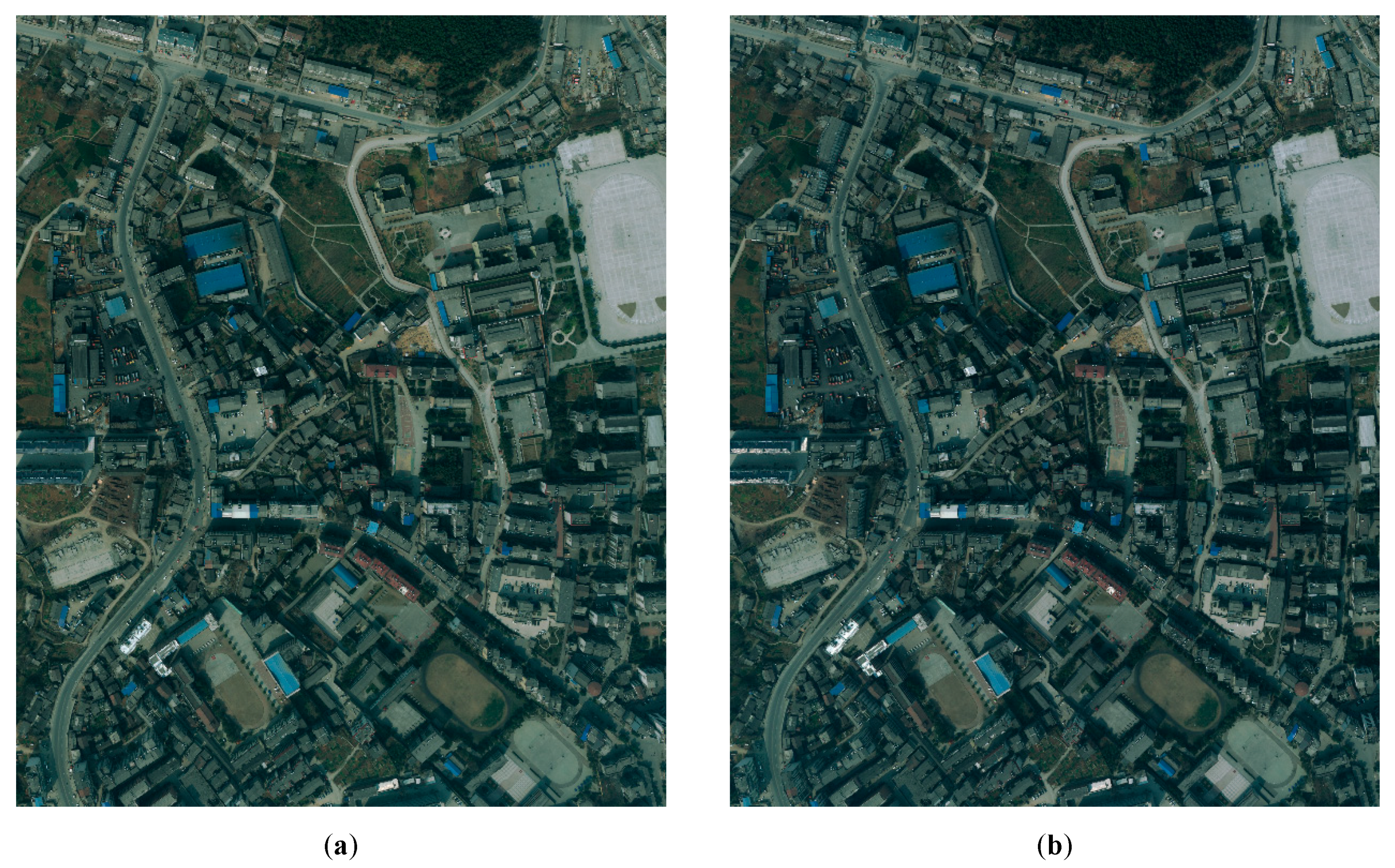
| Dataset A | 0.5 | 3030 × 2067 × 3 | Central area of a big city |
| Dataset B | 0.2 | 2438 × 4824 × 3 | Suburb of a big city |
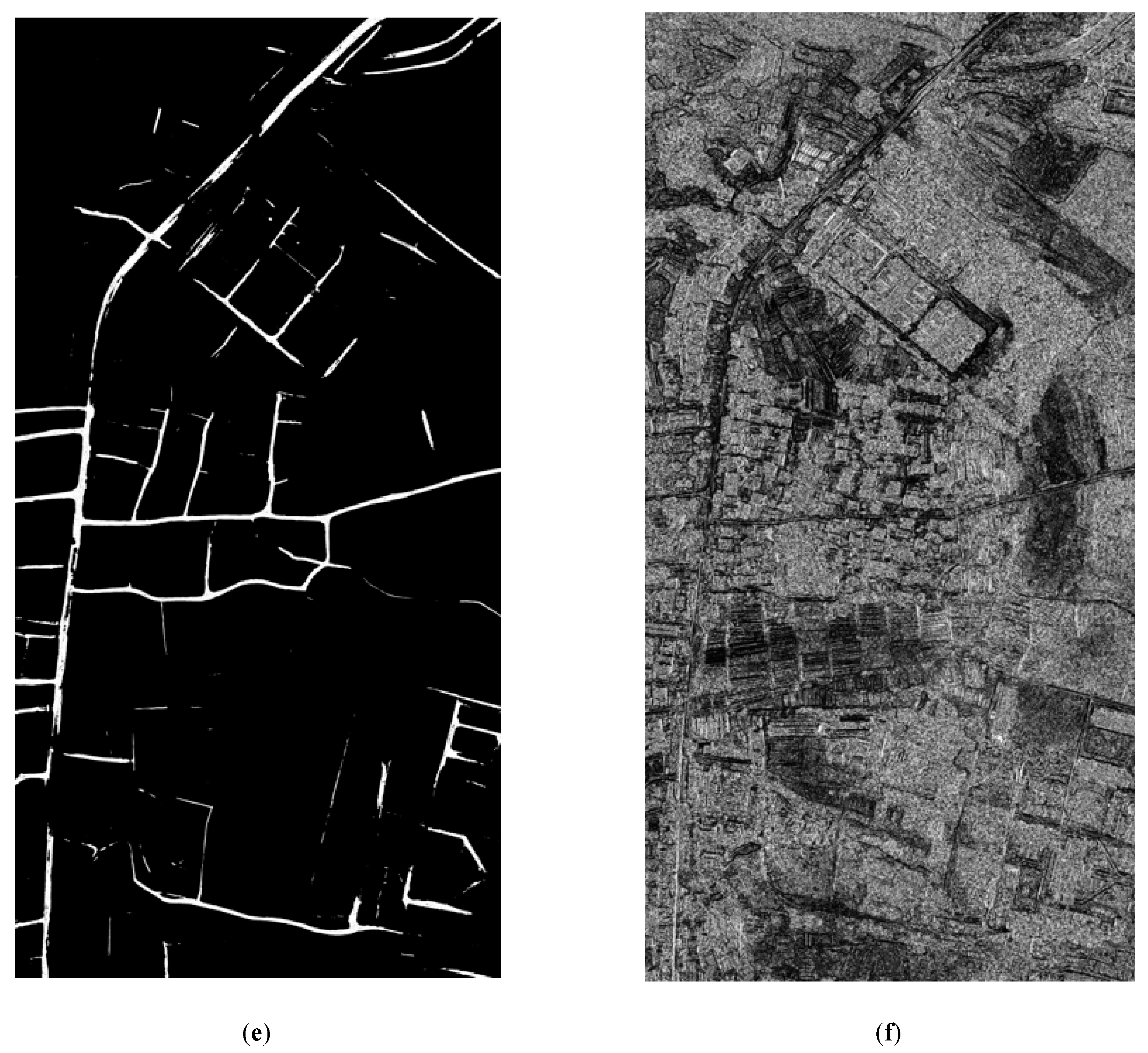
| Dataset C | 0.3 | 2212 × 2693 × 3 | Central area of a medium-sized city |
| Dataset | Method | Number of Obvious Objects Passed Through | Processing Time (s) |
|---|---|---|---|
| 1 | Dijkstra’s | 5 | 329.770 |
| OrthoVista | 9 | 13.000 | |
| Proposed | 1 | 21.387+Δ | |
| Dijkstra’s | 6 | 1033.976 | |
| 2 | OrthoVista | 6 | 21.000 |
| Proposed | 0 | 38.353+Δ | |
| Dijkstra’s | 2 | 568.329 | |
| 3 | OrthoVista | 11 | 9.000 |
| Proposed | 2 | 8.612+Δ |
| The Values of w | Number of Obvious Objects Passed Through | Processing Time (s) |
|---|---|---|
| 0.1 | 11 | 24.522+Δ |
| 0.01 | 4 | 18.602+Δ |
| 0.001 | 1 | 21.387+Δ |
| 0.0001 | 1 | 25.461+Δ |
| 0.00001 | 1 | 25.491+Δ |
© 2020 by the authors. Licensee MDPI, Basel, Switzerland. This article is an open access article distributed under the terms and conditions of the Creative Commons Attribution (CC BY) license (http://creativecommons.org/licenses/by/4.0/).
Share and Cite
Yuan, S.; Yang, K.; Li, X.; Cai, H. Automatic Seamline Determination for Urban Image Mosaicking Based on Road Probability Map from the D-LinkNet Neural Network. Sensors 2020, 20, 1832. https://doi.org/10.3390/s20071832
Yuan S, Yang K, Li X, Cai H. Automatic Seamline Determination for Urban Image Mosaicking Based on Road Probability Map from the D-LinkNet Neural Network. Sensors. 2020; 20(7):1832. https://doi.org/10.3390/s20071832
Chicago/Turabian StyleYuan, Shenggu, Ke Yang, Xin Li, and Hongyue Cai. 2020. "Automatic Seamline Determination for Urban Image Mosaicking Based on Road Probability Map from the D-LinkNet Neural Network" Sensors 20, no. 7: 1832. https://doi.org/10.3390/s20071832
APA StyleYuan, S., Yang, K., Li, X., & Cai, H. (2020). Automatic Seamline Determination for Urban Image Mosaicking Based on Road Probability Map from the D-LinkNet Neural Network. Sensors, 20(7), 1832. https://doi.org/10.3390/s20071832