A Learning-Enhanced Two-Pair Spatiotemporal Reflectance Fusion Model for GF-2 and GF-1 WFV Satellite Data

Abstract
1. Introduction
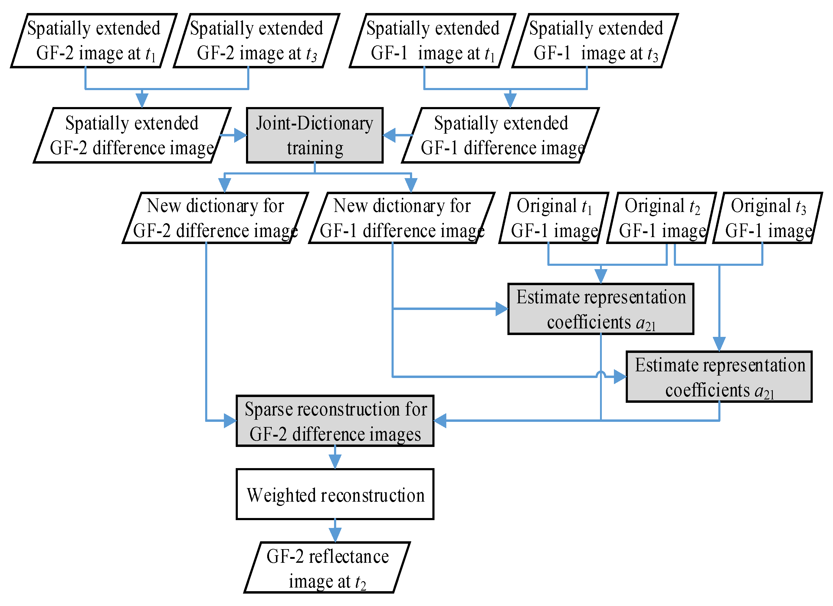
2. Methods
3. Results
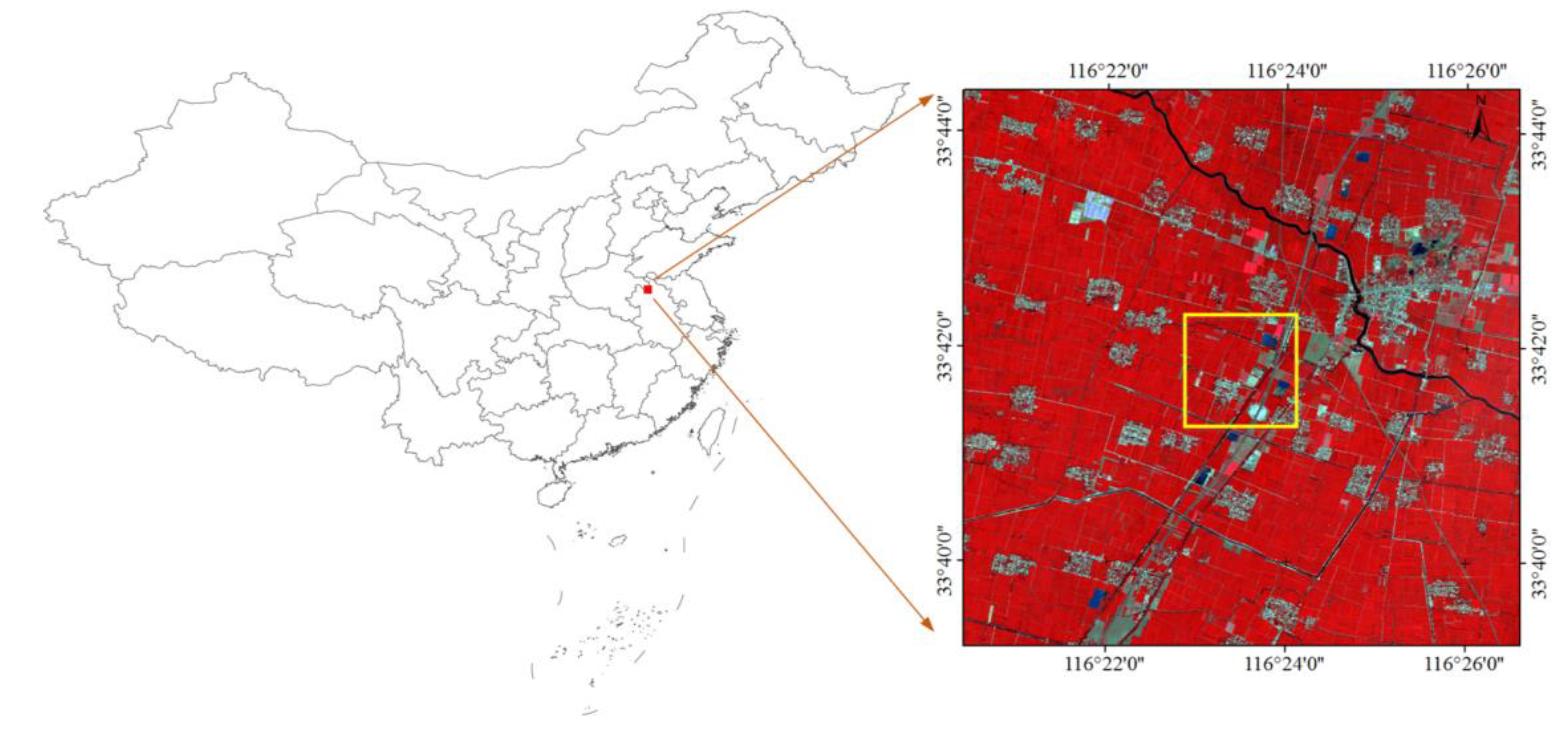
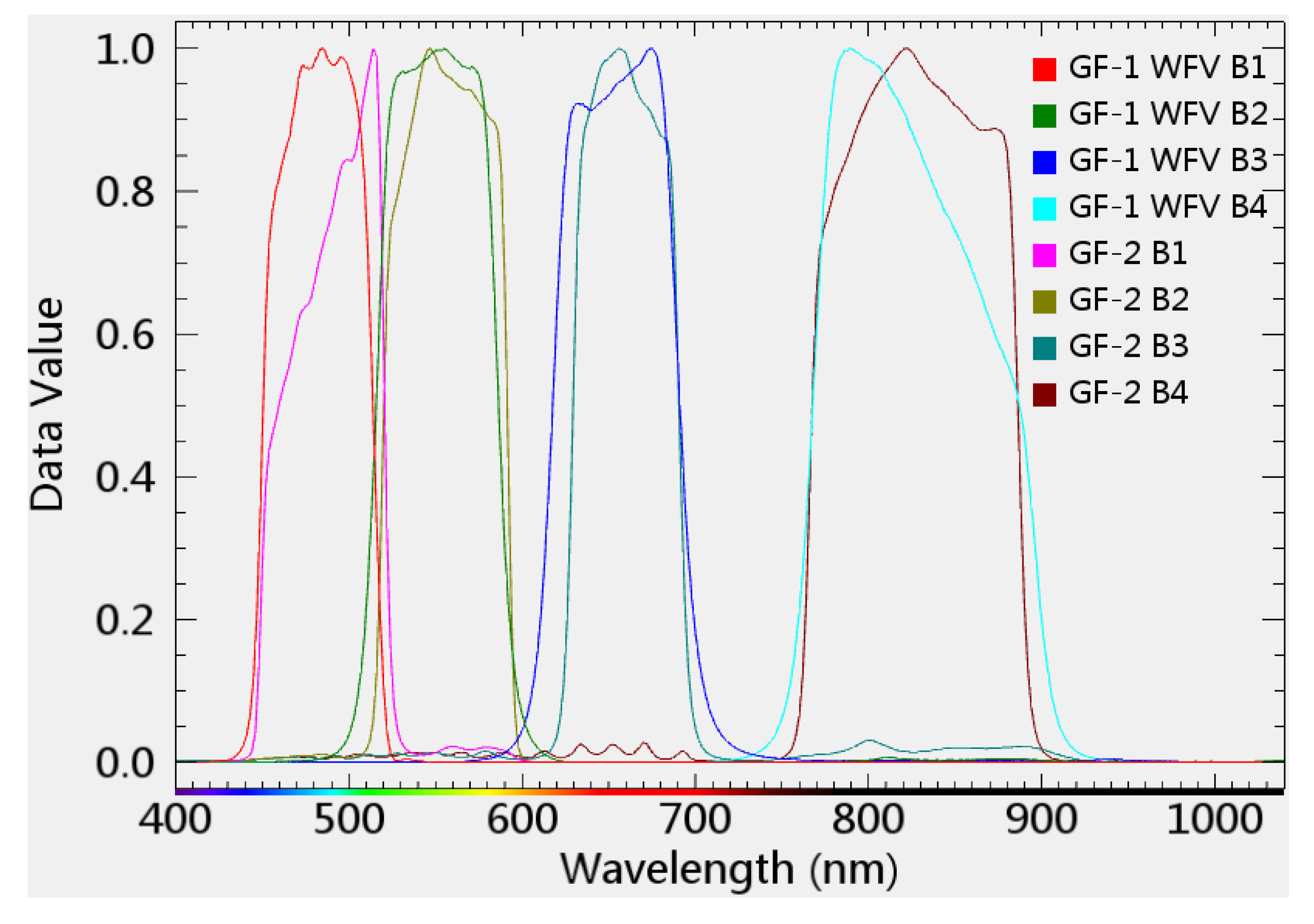
3.1. Study Area and Data Preprocessing
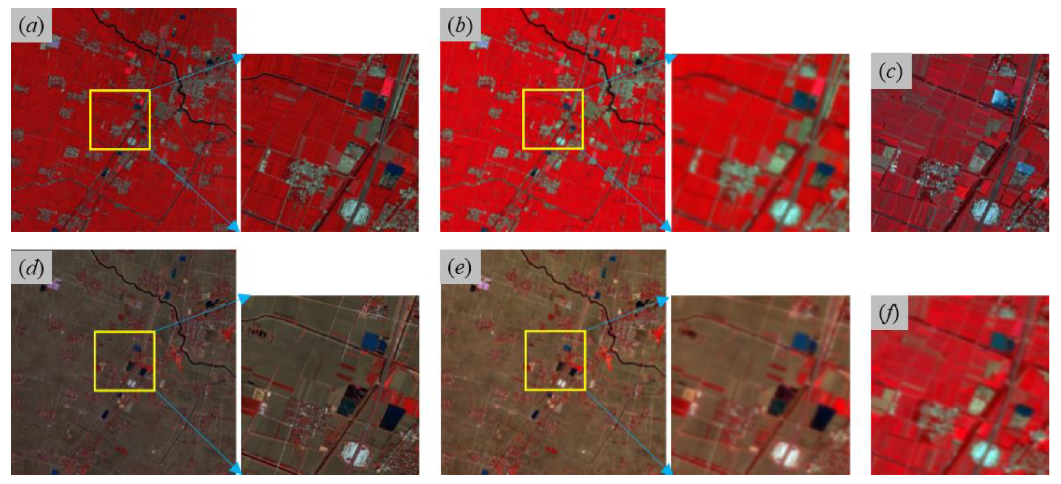
3.2. Experimental Results
4. Discussion
5. Conclusions
Author Contributions
Funding
Acknowledgments
Conflicts of Interest
References
- Tong, X. Development of China high-resolution earth observation system. J. Remote Sens. 2016, 20, 775–780. [Google Scholar]
- Han, Q.; Ma, L.; Liu, L.; Zhang, X.; Fu, Q.; Pan, Z.; Wang, A. On-Orbit Calibration and Evaluation of GF-2 Satellite Based on Wide Dynamic Ground Target. Acta Opt. Sin. 2015, 35, 0728003. [Google Scholar]
- Han, Q.; Fu, Q.; Zhang, X.; Liu, L. High-frequency radiometric calibration for wide field-of-view sensor of GF-1 satellite. Opt. Precis. Eng. 2014, 22, 1707–1714. [Google Scholar]
- Chen, B.; Huang, B.; Xu, B. Multi-s ource remotely sensed data fusion for improving land cover classification. ISPRS J. Photogramm. Remote Sens. 2017, 124, 27–39. [Google Scholar] [CrossRef]
- Shen, H.; Meng, X.; Zhang, L. An integrated framework for the spatio-temporal-spectral fusion of remote sensing images. IEEE Trans. Geosci. Remote Sens. 2016, 54, 7135–7148. [Google Scholar] [CrossRef]
- Chen, B.; Huang, B.; Xu, B. Comparison of spatiotemporal fusion models: A review. Remote Sens. 2015, 7, 1798–1835. [Google Scholar] [CrossRef]
- Zhang, L.; Shen, H. Progress and future of remote sensing data fusion. J. Remote Sens. 2016, 20, 1050–1061. [Google Scholar]
- Acerbi-Junior, F.W.; Clevers, J.G.P.W.; Schaepman, M.E. The assessment of multi-sensor image fusion using wavelet transforms for mapping the Brazilian Savanna. Int. J. Appl. Earth Obs. Geoinf. 2006, 8, 278–288. [Google Scholar] [CrossRef]
- Fortin, J.P.; Bernier, M.; Lapointe, S.; Gauthier, Y.; De Sève, D.; Beaudoin, S. Estimation of surface variables at the sub-pixel level for use as input to climate and hydrological models. Rapp. De Rech. Inrs-Eau 1998, 564, 64. [Google Scholar]
- Cherchali, S.; Amram, O.; Flouzat, G. Retrieval of temporal profiles of reflectances from simulated and real NOAA-AVHRR data over heterogeneous landscapes. Int. J. Remote Sens. 2000, 21, 753–775. [Google Scholar] [CrossRef]
- Zhukov, B.; Oertel, D.; Lanzl, F.; Reinhackel, G. Unmixing-based multisensor multiresolution image fusion. IEEE Trans. Geosci. Remote Sens. 1999, 37, 1212–1226. [Google Scholar] [CrossRef]
- Maselli, F. Definition of spatially variable spectral endmembers by locally calibrated multivariate regression analyses. Remote Sens. Environ. 2001, 75, 29–38. [Google Scholar] [CrossRef]
- Zhu, X.; Helmer, E.H.; Gao, F.; Liu, D.; Chen, J.; Lefsky, M.A. A flexible spatiotemporal method for fusing satellite images with different resolutions. Remote Sens. Environ. 2016, 172, 165–177. [Google Scholar] [CrossRef]
- Gao, F.; Masek, J.; Schwaller, M.; Hall, F. On the blending of the Landsat and MODIS surface reflectance: Predicting daily Landsat surface reflectance. IEEE Trans. Geosci. Remote Sens. 2006, 44, 2207–2218. [Google Scholar]
- Shen, H.; Wu, P.; Liu, Y.; Ai, T.; Wang, Y.; Liu, X. A spatial and temporal reflectance fusion model considering sensor observation differences. Int. J. Remote Sens. 2013, 34, 4367–4383. [Google Scholar] [CrossRef]
- Liu, F.; Wang, Z. Synthetic Landsat data through data assimilation for winter wheat yield estimation. In Proceedings of the 18th International Conference on Geoinformatics, Beijing, China, 18–20 June 2010. [Google Scholar]
- Anderson, M.C.; Kustas, W.P.; Norman, J.M.; Hain, C.R.; Mecikalski, J.R.; Schultz, L.; González-Dugo, M.P.; Cammalleri, C.; d’Urso, G.; Pimstein, A.; et al. Mapping daily evapotranspiration at field to continental scales using geostationary and polar orbiting satellite imagery. Hydrol. Earth Syst. Sci. 2011, 15, 223–239. [Google Scholar] [CrossRef]
- Gaulton, R.; Hilker, T.; Wulder, M.A.; Coops, N.C.; Stenhouse, G. Characterizing stand-replacing disturbance in western Alberta grizzly bear habitat, using a satellite-derived high temporal and spatial resolution change sequence. For. Ecol. Manag. 2011, 261, 865–877. [Google Scholar] [CrossRef]
- Walker, J.J.; de Beurs, K.M.; Wynne, R.H.; Gao, F. Evaluation of Landsat and MODIS data fusion products for analysis of dryland forest phenology. Remote Sens. Environ. 2012, 117, 381–393. [Google Scholar] [CrossRef]
- Bhandari, S.; Phinn, S.; Gill, T. Preparing Landsat image time series (LITS) for monitoring changes in vegetation phenology in Queensland, Australia. Remote Sens. 2012, 4, 1856–1886. [Google Scholar] [CrossRef]
- Singh, D. Generation and evaluation of gross primary productivity using Landsat data through blending with MODIS data. Int. J. Appl. Earth Obs. Geoinf. 2011, 13, 59–69. [Google Scholar] [CrossRef]
- Watts, J.D.; Powell, S.L.; Lawrence, R.L.; Hilker, T. Improved classification of conservation tillage adoption using high temporal and synthetic satellite imagery. Remote Sens. Environ. 2011, 115, 66–75. [Google Scholar] [CrossRef]
- Zhong, L.H.; Gong, P.; Biging, G.S. Phenology-based crop classification algorithm and its implications on agricultural water use assessments in California’s Central Valley. Photogramm. Eng. Remote Sens. 2012, 78, 799–813. [Google Scholar] [CrossRef]
- Liu, H.; Weng, Q.H. Enhancing temporal resolution of satellite imagery for public health studies: A case study of West Nile virus outbreak in Los Angeles in 2007. Remote Sens. Environ. 2012, 117, 57–71. [Google Scholar] [CrossRef]
- Zhu, X.; Chen, J.; Gao, F.; Chen, X.; Masek, J.G. An enhanced spatial and temporal adaptive reflectance fusion model for complex heterogeneous regions. Remote Sens. Environ. 2010, 114, 2610–2623. [Google Scholar] [CrossRef]
- Michishita, R.; Jiang, Z.; Gong, P.; Xu, B. Bi-scale analysis of multitemporal land cover fractions for wetland vegetation mapping. ISPRS J. Photogramm. Remote Sens. 2012, 72, 1–15. [Google Scholar] [CrossRef]
- Zhu, X.; Cai, F.; Tian, J.; Williams, T.K.A. Spatiotemporal fusion of multisource remote sensing data: Literature survey, taxonomy, principles, applications, and future directions. Remote Sens. 2018, 10, 527. [Google Scholar]
- Roy, D.P.; Ju, J.; Lewis, P.; Schaaf, C.; Gao, F.; Hansen, M.; Lindquist, E. Multi-temporal MODIS-Landsat data fusion for relative radiometric normalization, gap filling, and prediction of Landsat data. Remote Sens. Environ. 2008, 112, 3112–3130. [Google Scholar] [CrossRef]
- Li, D.; Tang, P.; Hu, C.; Zheng, K. Spatial-temporal fusion algorithm based on an extended semi-physical model and its preliminary application. J. Remote Sens. 2014, 18, 307–319. [Google Scholar]
- Wang, Q.; Atkinson, P.M. Spatio-temporal fusion for daily Sentinel-2 images. Remote Sens. Environ. 2018, 204, 31–42. [Google Scholar] [CrossRef]
- Song, H.; Huang, B. Spatiotemporal satellite image fusion through one-pair image learning. IEEE Trans. Geosci. Remote Sens. 2013, 51, 1883–1896. [Google Scholar] [CrossRef]
- Huang, B.; Song, H. Spatiotemporal reflectance fusion via sparse representation. IEEE Trans. Geosci. Remote Sens. 2012, 50, 3707–3716. [Google Scholar] [CrossRef]
- Liu, X.; Deng, C.; Wang, S.; Huang, G.B.; Zhao, B.; Lauren, P. Fast and accurate spatiotemporal fusion based upon extreme learning machine. IEEE Geosci. Remote Sens. Lett. 2016, 13, 2039–2043. [Google Scholar] [CrossRef]
- Li, D.; Li, Y.; Yang, W.; Ge, Y.; Han, Q.; Ma, L.; Chen, Y.; Li, X. An Enhanced Single-Pair Learning-Based Reflectance Fusion Algorithm with Spatiotemporally Extended Training Samples. Remote Sens. 2018, 10, 1207–1226. [Google Scholar] [CrossRef]
- Yuhas, R.H.; Goetz, A.F.H.; Boardman, J.W. Discrimination among semi-arid landscape endmembers using the spectral angle mapper (SAM) algorithm. In Proceedings of the Summaries of the Third Annual JPL Airborne Geoscience Workshop, Pasadena, CA, USA, 1–5 June 1992; pp. 147–149. [Google Scholar]
- Wang, Z.; Bovik, A.C.; Sheikh, H.R.; Simoncelli, E.P. Image quality assessment: From error visibility to structural similarity. IEEE Trans. Image Process. 2004, 13, 600–612. [Google Scholar] [CrossRef] [PubMed]
- Renza, D.; Martinez, E.; Arquero, A. A new approach to change detection in multispectral images by means of ERGAS index. IEEE Geosci. Remote Sens. Lett. 2013, 10, 76–80. [Google Scholar] [CrossRef]
- Aharon, M.; Elad, M.; Bruckstein, A.M. The K-SVD: An Algorithm for Designing of Overcomplete Dictionaries for Sparse Representation. IEEE Trans. Image Process. 2006, 54, 4311–4322. [Google Scholar] [CrossRef]
- Rubinstein, R.; Zibulevsky, M.; Elad, M. Efficient Implementation of the K-SVD Algorithm Using Batch Orthogonal Matching Pursuit. Computer Science Department Technion. Rep. 2008. Available online: http://www.cs.technion.ac.il/users/wwwb/cgi-bin/tr-get.cgi/2008/CS/CS-2008-08.pdf (accessed on 21 March 2020).


| Band Name | GF-2 Multispectral | GF-1 WFV | ||||||
|---|---|---|---|---|---|---|---|---|
| Band Width | Spatial Resolution | Revisit Cycle | Employed Dates | Band Width | Spatial Resolution | Revisit Cycle | Employed Dates | |
| Blue | 0.45–0.52 μm | 4 m | 5 days | 04/30/2017 07/23/2017 11/08/2017 | 0.45–0.52 μm | 16 m | 2 days | 04/29/2017 07/24/2017 11/08/2017 |
| Green | 0.52–0.59 μm | 0.52–0.59 μm | ||||||
| Red | 0.63–0.69 μm | 0.63–0.69 μm | ||||||
| NIR | 0.77–0.89 μm | 0.77–0.89 μm | ||||||
| Methods | Training Sample Size | AAD × 102 | PSNR | CC | ERGAS | ||||||
|---|---|---|---|---|---|---|---|---|---|---|---|
| Green | Red | NIR | Green | Red | NIR | Green | Red | NIR | |||
| SPSTFM | 500 × 500 | 1.67 | 1.58 | 4.72 | 23.9890 | 23.9886 | 20.6887 | 0.8348 | 0.8206 | 0.6978 | 30.2124 |
| Proposed fusion model | 600 × 600 | 1.54 | 1.57 | 4.69 | 23.7903 | 24.2777 | 20.9278 | 0.8391 | 0.8358 | 0.7146 | 28.9806 |
| 700 × 700 | 1.49 | 1.55 | 4.64 | 23.6544 | 24.4698 | 21.3056 | 0.8445 | 0.8380 | 0.7227 | 27.5489 | |
| 800 × 800 | 1.44 | 1.52 | 4.58 | 23.3901 | 24.6415 | 21.5419 | 0.8489 | 0.8447 | 0.7266 | 28.1647 | |
| 900 × 900 | 1.44 | 1.50 | 4.53 | 23.2203 | 24.9902 | 21.6763 | 0.8533 | 0.8493 | 0.7304 | 26.5306 | |
| 1000 × 1000 | 1.40 | 1.49 | 3.49 | 23.1411 | 25.1369 | 21.8535 | 0.8550 | 0.8525 | 0.7341 | 26.1852 | |
| 1100 × 1100 | 1.37 | 1.47 | 3.45 | 24.0155 | 25.4554 | 22.0025 | 0.8582 | 0.8566 | 0.7369 | 25.9577 | |
| 1200 × 1200 | 1.36 | 1.46 | 3.37 | 24.1223 | 25.5109 | 22.3117 | 0.8597 | 0.8584 | 0.7397 | 24.5226 | |
| 1300 × 1300 | 1.33 | 1.43 | 3.30 | 24.3005 | 25.6688 | 22.7006 | 0.8623 | 0.8631 | 0.7434 | 25.0774 | |
| 1400 × 1400 | 1.28 | 1.44 | 3.25 | 24.4379 | 25.6979 | 22.8990 | 0.8644 | 0.8679 | 0.7482 | 23.4095 | |
| 1500 × 1500 | 1.25 | 1.41 | 3.11 | 24.7706 | 25.7452 | 23.1453 | 0.8679 | 0.8694 | 0.7527 | 23.1710 | |
| 1600 × 1600 | 1.24 | 1.39 | 2.81 | 24.8269 | 25.7885 | 23.3366 | 0.8688 | 0.8728 | 0.7573 | 23.0139 | |
| 1700 × 1700 | 1.22 | 1.37 | 2.72 | 24.9901 | 25.8503 | 23.4210 | 0.8702 | 0.8755 | 0.7610 | 23.8441 | |
| 1800 × 1800 | 1.19 | 138 | 2.70 | 25.1796 | 25.9116 | 23.6962 | 0.8731 | 0.8771 | 0.7644 | 23.2267 | |
| 1900 × 1900 | 1.18 | 1.36 | 2.67 | 25.3661 | 25.9820 | 23.8331 | 0.8756 | 0.8797 | 0.7697 | 22.9553 | |
| 2000 × 2000 | 1.18 | 1.34 | 2.66 | 25.4157 | 25.9833 | 23.8400 | 0.8754 | 0.8800 | 0.7711 | 22.9874 | |
| STARFM | — | 1.75 | 1.56 | 4.38 | 23.5678 | 24.1568 | 20.6543 | 0.8533 | 0.8496 | 0.7301 | 26.0771 |
| ESTARFM | — | 1.69 | 1.47 | 3.53 | 23.4508 | 24.3378 | 21.6888 | 0.8384 | 0.8517 | 0.7009 | 25.9248 |
| Methods | Training Sample size | RMSE ×102 | SAM | SSIM × 102 | Elapsed Time (s) | ||||||
| Green | Red | NIR | Green | Red | NIR | Green | Red | NIR | |||
| SPSTFM | 500 × 500 | 2.41 | 3.36 | 6.47 | 1.7829 | 1.7880 | 1.8993 | 87.08 | 73.61 | 61.18 | 60.95 |
| Proposed fusion model | 600 × 600 | 2.29 | 3.21 | 6.29 | 1.7863 | 1.7563 | 1.8563 | 87.94 | 83.94 | 67.94 | 67.59 |
| 700 × 700 | 2.22 | 3.17 | 6.31 | 1.7855 | 1.7655 | 1.8109 | 88.17 | 84.57 | 71.17 | 88.26 | |
| 800 × 800 | 2.31 | 2.94 | 5.86 | 1.7745 | 1.7445 | 1.8245 | 87.34 | 85.46 | 72.46 | 91.75 | |
| 900 × 900 | 2.15 | 2.85 | 5.45 | 1.7833 | 1.7492 | 1.8133 | 88.26 | 86.34 | 73.34 | 96.30 | |
| 1000 × 1000 | 2.10 | 2.77 | 5.38 | 1.7790 | 1.7543 | 1.8046 | 88.42 | 87.09 | 75.07 | 110.17 | |
| 1100 × 1100 | 2.23 | 2.63 | 5.29 | 1.7811 | 1.7415 | 1.7811 | 89.33 | 87.98 | 74.82 | 122.63 | |
| 1200 × 1200 | 2.19 | 2.49 | 5.31 | 1.7794 | 1.6893 | 1.7914 | 89.92 | 88.44 | 74.69 | 135.76 | |
| 1300 × 1300 | 2.15 | 2.51 | 5.15 | 1.7807 | 1.6780 | 1.8087 | 89.77 | 88.17 | 74.57 | 166.44 | |
| 1400 × 1400 | 2.16 | 2.36 | 4.91 | 1.7765 | 1.6884 | 1.7947 | 89.89 | 89.29 | 75.92 | 179.28 | |
| 1500 × 1500 | 2.01 | 2.27 | 4.84 | 1.7636 | 1.6731 | 1.7882 | 90.18 | 89.42 | 76.34 | 201.16 | |
| 1600 × 1600 | 2.01 | 2.25 | 4.86 | 1.7679 | 1.7379 | 1.8009 | 90.14 | 89.64 | 76.64 | 227.81 | |
| 1700 × 1700 | 2.02 | 2.31 | 4.90 | 1.7685 | 1.7475 | 1.7852 | 90.07 | 88.83 | 75.89 | 250.66 | |
| 1800 × 1800 | 2.01 | 2.27 | 4.84 | 1.7521 | 1.7551 | 1.7801 | 90.10 | 89.25 | 76.41 | 279.05 | |
| 1900 × 1900 | 2.03 | 2.24 | 4.91 | 1.7469 | 1.7460 | 1.7767 | 90.16 | 89.71 | 76.16 | 311.68 | |
| 2000 × 2000 | 2.02 | 2.22 | 4.88 | 1.7514 | 1.7471 | 1.7823 | 90.18 | 90.06 | 76.81 | 323.44 | |
| STARFM | — | 2.40 | 2.45 | 5.50 | 1.7812 | 1.7605 | 1.8181 | 87.22 | 87.47 | 75.19 | 10.78 |
| ESTARFM | — | 2.41 | 2.48 | 5.02 | 1.7749 | 1.7538 | 1.8126 | 85.80 | 86.36 | 70.27 | 348.56 |
© 2020 by the authors. Licensee MDPI, Basel, Switzerland. This article is an open access article distributed under the terms and conditions of the Creative Commons Attribution (CC BY) license (http://creativecommons.org/licenses/by/4.0/).
Share and Cite
Ge, Y.; Li, Y.; Chen, J.; Sun, K.; Li, D.; Han, Q. A Learning-Enhanced Two-Pair Spatiotemporal Reflectance Fusion Model for GF-2 and GF-1 WFV Satellite Data. Sensors 2020, 20, 1789. https://doi.org/10.3390/s20061789
Ge Y, Li Y, Chen J, Sun K, Li D, Han Q. A Learning-Enhanced Two-Pair Spatiotemporal Reflectance Fusion Model for GF-2 and GF-1 WFV Satellite Data. Sensors. 2020; 20(6):1789. https://doi.org/10.3390/s20061789
Chicago/Turabian StyleGe, Yanqin, Yanrong Li, Jinyong Chen, Kang Sun, Dacheng Li, and Qijin Han. 2020. "A Learning-Enhanced Two-Pair Spatiotemporal Reflectance Fusion Model for GF-2 and GF-1 WFV Satellite Data" Sensors 20, no. 6: 1789. https://doi.org/10.3390/s20061789
APA StyleGe, Y., Li, Y., Chen, J., Sun, K., Li, D., & Han, Q. (2020). A Learning-Enhanced Two-Pair Spatiotemporal Reflectance Fusion Model for GF-2 and GF-1 WFV Satellite Data. Sensors, 20(6), 1789. https://doi.org/10.3390/s20061789