Modern Soft-Sensing Modeling Methods for Fermentation Processes


Abstract
1. Introduction
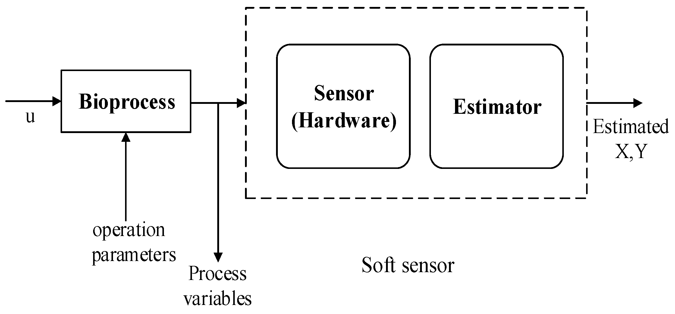
2. Soft Sensor
3. Soft Sensor Development Methodology
3.1. Data collection and Pre-Processing
3.2. Selection of Variables
3.3. Soft Sensor Model Selection, Training and Validation
3.4. Performance Evaluation of Soft Sensor Model
3.5. Use Case Implementation of Soft Sensor
4. Review of Modern Soft-Sensing Models and Optimization Techniques
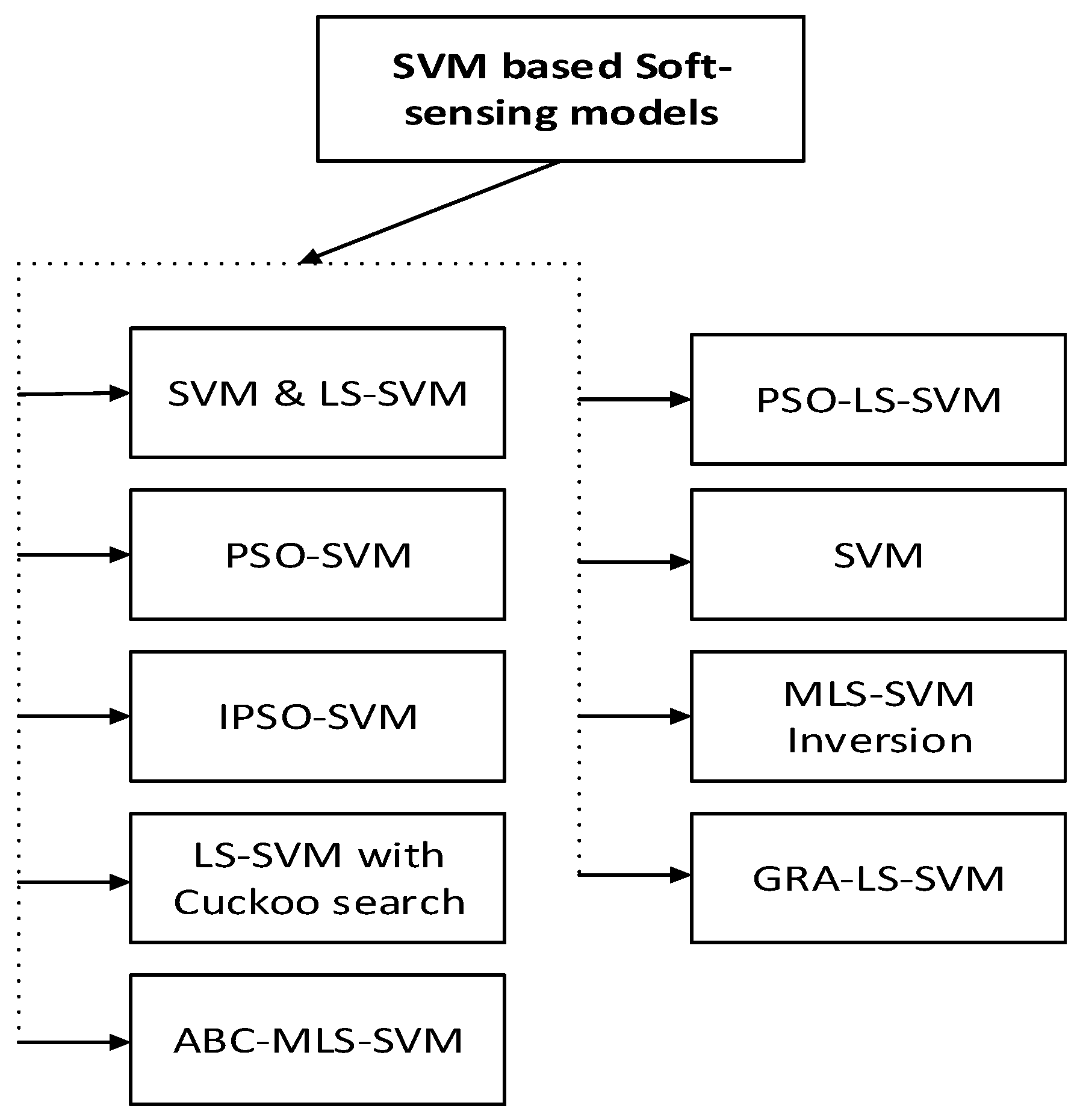
4.1. Support Vector Machine-Based Soft-Sensing Models
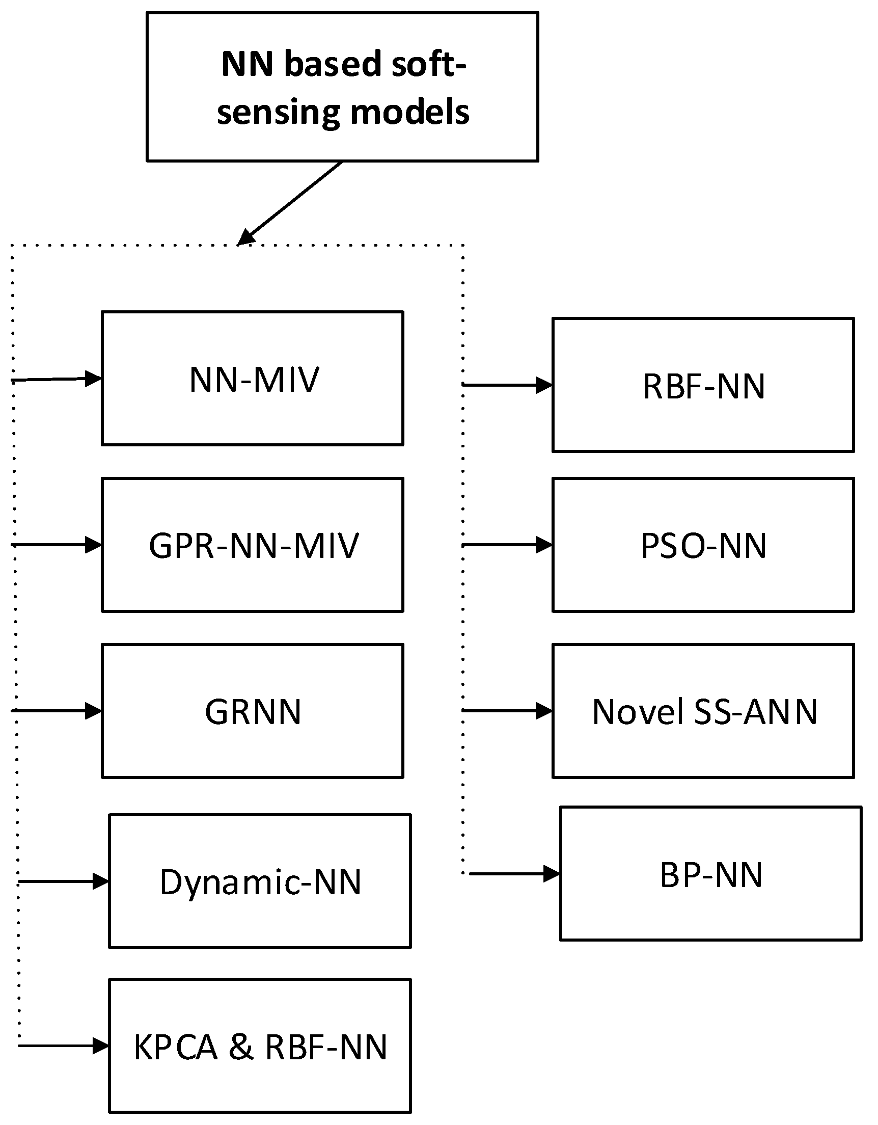
4.2. Neural Network-Based Soft-Sensing Models
4.3. Deep Learning Based Soft-Sensing Models
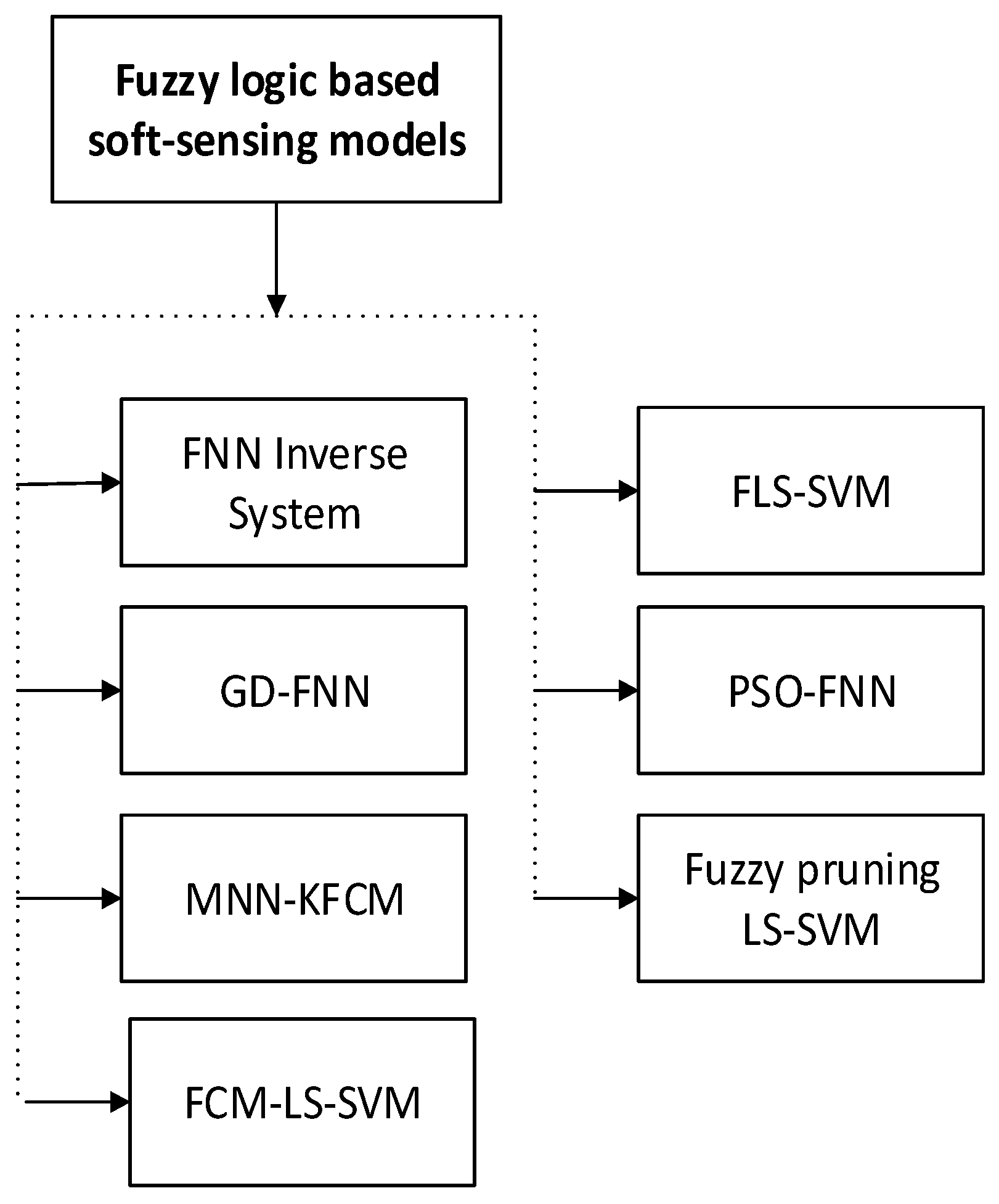
4.4. Fuzzy Logic Based Soft-Sensing Models
4.5. Genetic Algorithm-Based Soft Sensors
4.6. Probabilistic Latent Variable Modeling Methods
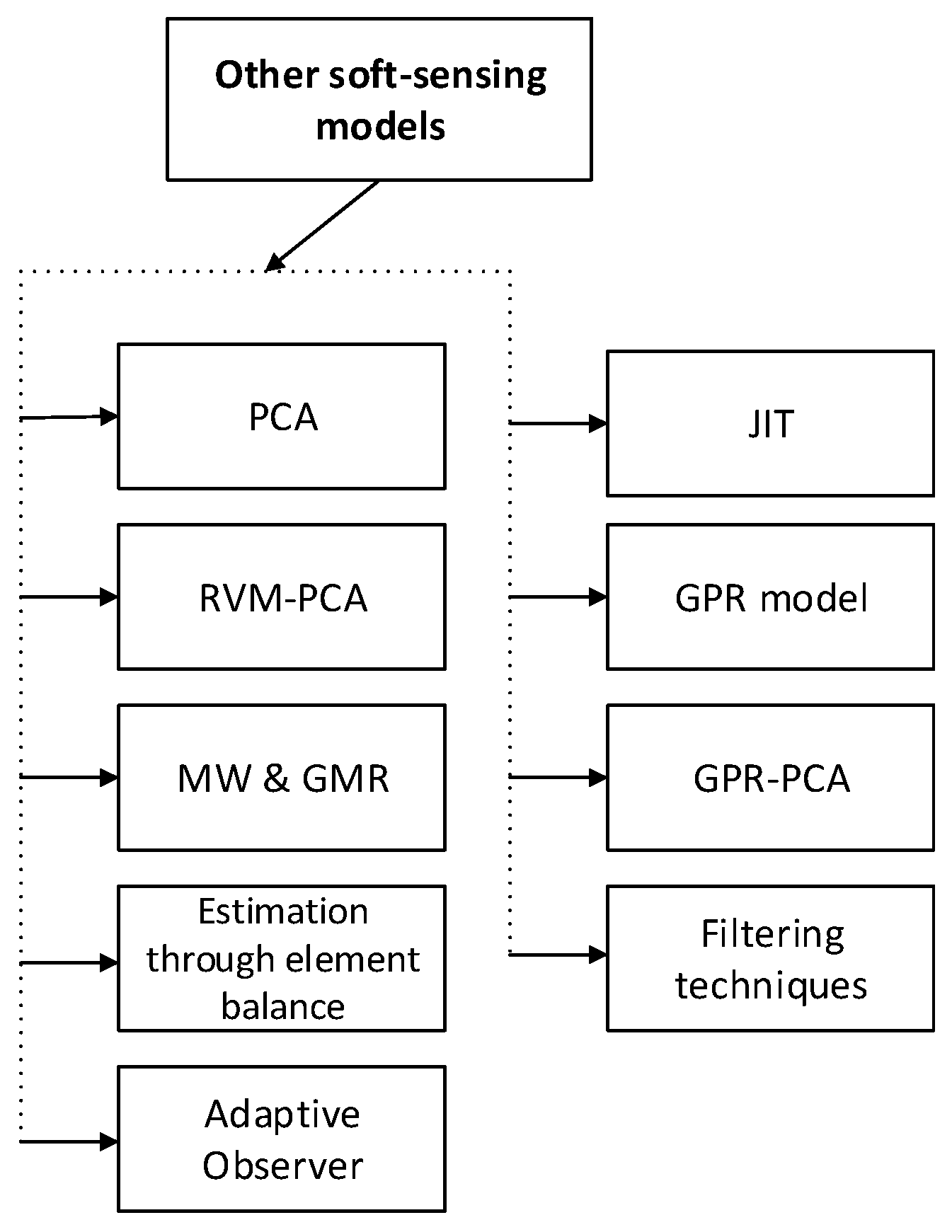
4.7. Other Useful Methods
- Filtering techniques, estimation through element balance and adaptive observer [112].
- Relevance vector machine (RVM) based on the PCA algorithm for fermentation [113].
- Gaussian mixture regression (GMR)-based soft-sensing modeling method presented in [114].
- Soft-sensing modeling methods based on multi-model adaptive by using local learning and online SVR for non-linear time-variant batch processes [115].
- Just-in-time (JIT) modeling with a combination of input and output similarity criteria for the soft-sensing modeling in fermentation processes [116].
- Dual learning-based online ensemble regression approach for adaptive soft-sensing modeling of nonlinear time-varying processes [117].
- A soft-sensing model based on GPR for the erythromycin fermentation process is presented in [118].
- A soft-sensing modeling method based on multi-model strategy by using GPR and PCA is presented in [119].
- A soft-sensing modeling method for product concentration monitoring in a fed-batch fermentation process based on dynamic principal component regression PCR proposed in [120].
5. Optimization Techniques
6. Comparative Analysis
7. Conclusions and Future Perspective
Author Contributions
Funding
Ethical Approval
Conflicts of Interest
Appendix A

| Abbreviation | Explanation |
|---|---|
| Methods | |
| SVM | Support Vector Machines |
| SVR | Support Vector Regression |
| LS-SVM | Least Square Support Vector Machine |
| PLS | Partial Least Squares |
| MLS-SVM | Multiple Output Least Squares Support Vector Machine |
| MSE | Mean Square Error |
| RMSE | Root Mean Square Error |
| NN | Neural Network |
| DNN | Deep Neural Network |
| ANN | Artificial Neural Network |
| DL | Deep Learning |
| NLP | Natural Language Processing |
| DAE | Denoising auto-encoders |
| SAE | Stacking auto-encoders |
| HELM | Hierarchical Extreme Learning Machine |
| MIV | Mean Impact Value |
| BPNN | Back-propagation Neural Network |
| RBF | Radial Basis Function |
| GPC | Generalized Predictive Control |
| PID | Proportional-Integral-Derivative |
| GRA | Gray Relational Analysis |
| PSO | Particle Swarm Optimization |
| IPSO | Improved Particle Swarm Optimization |
| ABC | Artificial Bee Colony |
| ACO | Ant colony optimization |
| CS | Cuckoo Search |
| GA | Genetic Algorithm |
| KNN | K-nearest Neighbors |
| GPR | Gaussian Process Regression |
| GRNN | Generalized Regression Neural Network |
| KPCA | Kernel Principal Component Analysis |
| PCA | Principal Component Analysis |
| ICA | Independent Component Analysis |
| FL | Fuzzy Logic |
| FNN | Fuzzy Neural Network |
| GD-FNN | Generalized Dynamic Fuzzy Neural Network |
| MNN | Multi-model Neural Network |
| KFCM | Kernel Fuzzy c-means Clustering |
| FLS | Fuzzy Least Square |
| FCM | Fuzzy c-means Clustering |
| AIC | Akaike information criterion |
| PLVM | Probabilistic Latent Variable Models |
| RVM | Relevance vector machine |
| GMR | Gaussian Mixture Regression |
| JIT | Just-In-Time |
| PCR | Principal Component Regression |
| AHP | Analytic Hierarchy Process |
References
- Buchholz, K.; Collins, J. The roots—A short history of industrial microbiology and biotechnology. Appl. Microbiol. Biotechnol. 2013, 97, 3747–3762. [Google Scholar] [CrossRef] [PubMed]
- Jelali, M. An overview of control performance assessment technology and industrial applications. Control Eng. Pract. 2006, 14, 441–466. [Google Scholar] [CrossRef]
- Alasalvar, C.; Miyashita, K.; Shahidi, F.; Wanasundara, U. Handbook of Seafood Quality, Safety and Health Applications; John Wiley & Sons: Hoboken, NJ, USA, 2011. [Google Scholar]
- Meihong, Z. Research Progress on the Medical Field of Marine Proteinases. Shandong Chem. Ind. 2016, 45, 60–63. [Google Scholar]
- Ren, X.; Hu, Y.; Hu, Q.; Yang, S.; Yu, H.; Zhen, G.; Yang, Z. Application of lysozyme in preservation of aquatic products. Sci.Technol. Food Ind. 2013, 34, 390–394. [Google Scholar]
- Kadlec, P.; Gabrys, B.; Strandt, S. Data-driven soft sensors in the process industry. Comput. Chem. Eng. 2009, 33, 795–814. [Google Scholar] [CrossRef]
- Luttmann, R.; Bracewell, D.G.; Cornelissen, G.; Gernaey, K.V.; Glassey, J.; Hass, V.C.; Kaiser, C.; Preusse, C.; Striedner, G.; Mandenius, C.F. Soft sensors in bioprocessing: A status report and recommendations. Biotechnol. J. 2012, 7, 1040–1048. [Google Scholar] [CrossRef]
- Fortuna, L.; Graziani, S.; Rizzo, A.; Xibilia, M.G. Soft Sensors for Monitoring and Control of Industrial Processes; Springer Science & Business Media: Berlin, Germany, 2007. [Google Scholar]
- Yan, W.; Tang, D.; Lin, Y. A data-driven soft sensor modeling method based on deep learning and its application. IEEE Trans. Ind. Electron. 2016, 64, 4237–4245. [Google Scholar] [CrossRef]
- Chéruy, A. Software sensors in bioprocess engineering. J. Biotechnol. 1997, 52, 193–199. [Google Scholar] [CrossRef]
- Chollet, F. Deep Learning mit Python und Keras: Das Praxis-Handbuch vom Entwickler der Keras-Bibliothek; MITP-Verlags GmbH & Co. KG: Frechen, Germany, 2018. [Google Scholar]
- Hastie, T.; Tibshirani, R.; Friedman, J. The elements of statistical learning. In Springer Series in Statistics; Springer: Berlin/Heidelberg, Germany, 2001. [Google Scholar]
- Andridge, R.R.; Little, R.J. A review of hot deck imputation for survey non-response. Int. Stat. Rev. 2010, 78, 40–64. [Google Scholar] [CrossRef]
- Enders, C.K. A primer on maximum likelihood algorithms available for use with missing data. Struct. Equ. Model. 2001, 8, 128–141. [Google Scholar] [CrossRef]
- Jerez, J.M.; Molina, I.; García-Laencina, P.J.; Alba, E.; Ribelles, N.; Martín, M.; Franco, L. Missing data imputation using statistical and machine learning methods in a real breast cancer problem. Artif. Intell. Med. 2010, 50, 105–115. [Google Scholar] [CrossRef]
- Pearson, R.K. Outliers in process modeling and identification. IEEE Trans. Control Syst. Technol. 2002, 10, 55–63. [Google Scholar] [CrossRef]
- Davies, L.; Gather, U. The identification of multiple outliers. J. Am. Stat. Assoc. 1993, 88, 782–792. [Google Scholar] [CrossRef]
- Liu, H.; Shah, S.; Jiang, W. On-line outlier detection and data cleaning. Comput. Chem. Eng. 2004, 28, 1635–1647. [Google Scholar] [CrossRef]
- Di Bella, A.; Fortuna, L.; Graziani, S.; Napoli, G.; Xibilia, M. A comparative analysis of the influence of methods for outliers detection on the performance of data driven models. In Proceedings of the 2007 IEEE Instrumentation & Measurement Technology Conference IMTC 2007, Warsaw, Poland, 1–3 May 2007; pp. 1–5. [Google Scholar]
- Warne, K.; Prasad, G.; Rezvani, S.; Maguire, L. Statistical and computational intelligence techniques for inferential model development: A comparative evaluation and a novel proposition for fusion. Eng. Appl. Artif. Intell. 2004, 17, 871–885. [Google Scholar] [CrossRef]
- Penny, K.I.; Jolliffe, I.T. A comparison of multivariate outlier detection methods for clinical laboratory safety data. J. R. Stat. Soc. Ser. D 2001, 50, 295–307. [Google Scholar] [CrossRef]
- Lee, H.W.; Lee, M.W.; Park, J.M. Robust adaptive partial least squares modeling of a full-scale industrial wastewater treatment process. Ind. Eng. Chem. Res. 2007, 46, 955–964. [Google Scholar] [CrossRef]
- Liu, Y.; Zhu, Z.; Zhu, X. Soft sensor modeling for key parameters of marine alkaline protease MP fermentation process. In Proceedings of the 2018 Chinese Control And Decision Conference (CCDC), Shenyang, China, 9–11 June 2018; pp. 6149–6154. [Google Scholar]
- Yonghong, H.; Hao, C.; Li, H.; Lina, S. Soft sensing modeling based on dynamic fuzzy neural network for penicillin fermentation. In Proceedings of the 31st Chinese Control Conference, Hefei, China, 23–25 May 2020; pp. 3383–3388. [Google Scholar]
- Fortuna, L.; Graziani, S.; Xibilia, M.G. Comparison of soft-sensor design methods for industrial plants using small data sets. IEEE Trans. Instrum. Meas. 2009, 58, 2444–2451. [Google Scholar] [CrossRef]
- Pani, A.K.; Mohanta, H.K. A survey of data treatment techniques for soft sensor design. Chem. Prod. Process Model. 2011, 6. [Google Scholar] [CrossRef]
- Gonzaga, J.; Meleiro, L.A.C.; Kiang, C.; Maciel Filho, R. ANN-based soft-sensor for real-time process monitoring and control of an industrial polymerization process. Comput. Chem. Eng. 2009, 33, 43–49. [Google Scholar] [CrossRef]
- Jolliffe, I.T. Principal components in regression analysis. In Principal component analysis; Springer: New York, NY, USA, 1986; pp. 129–155. [Google Scholar]
- Zamprogna, E.; Barolo, M.; Seborg, D.E. Optimal selection of soft sensor inputs for batch distillation columns using principal component analysis. J. Process Control 2005, 15, 39–52. [Google Scholar] [CrossRef]
- Guyon, I.; Elisseeff, A. An introduction to variable and feature selection. J. Mach. Learn. Res. 2003, 3, 1157–1182. [Google Scholar]
- Ding, Y.; Zeng, D.; Yang, P.; Liu, G.; Huang, Y.; Zhu, X. Soft sensor model of marine enzyme fermentation process based on NN-MIV variable selection. In Proceedings of the 2017 29th Chinese Control And Decision Conference (CCDC), Chongqing, China, 28–30 May 2017; pp. 6816–6820. [Google Scholar]
- Ge, Z. Process data analytics via probabilistic latent variable models: A tutorial review. Ind. Eng. Chem. Res. 2018, 57, 12646–12661. [Google Scholar] [CrossRef]
- Shang, C.; Yang, F.; Huang, D.; Lyu, W. Data-driven soft sensor development based on deep learning technique. J. Process Control 2014, 24, 223–233. [Google Scholar] [CrossRef]
- Yan, W.; Shao, H.; Wang, X. Soft sensing modeling based on support vector machine and Bayesian model selection. Comput. Chem. Eng. 2004, 28, 1489–1498. [Google Scholar] [CrossRef]
- Gösset, W. The probable error of a mean. Biometrika 1908, 6, 1–25. [Google Scholar]
- Brownlee, J. Deep Learning with Python: Develop Deep Learning Models on Theano and Tensorflow Using Keras; Machine Learning Mastery: Vermont, Australia, 2016. [Google Scholar]
- Hastie, T.; Tibshirani, R.; Friedman, J. The Elements of Statistical Learning: Data Mining, Inference, and Prediction; Springer Science & Business Media: Berlin, Germany, 2009. [Google Scholar]
- Ge, Z.; Liu, Y. Analytic hierarchy process based fuzzy decision fusion system for model prioritization and process monitoring application. Chemom. Intell. Lab. Syst. 2018, 15, 357–365. [Google Scholar] [CrossRef]
- Souza, F.A.; Araújo, R.; Mendes, J. Review of soft sensor methods for regression applications. Chemom. Intell. Lab. Syst. 2016, 152, 69–79. [Google Scholar] [CrossRef]
- LIN, B.; GU, X. Soft sensor modeling based on DE-LSSVM. J. Chem. Ind. Eng. (China) 2008, 7, 1681–1685. [Google Scholar]
- Wang, X.; Chen, J.; Liu, C.; Pan, F. Hybrid modeling of penicillin fermentation process based on least square support vector machine. Chem. Eng. Res. Des. 2010, 88, 415–420. [Google Scholar] [CrossRef]
- Jalel, N.; Shui, F.; Tsaptsinos, D.; Tang, R.; Vanichsriratana, W.; Leigh, J. Artificial intelligence in the control of a class of fermentation processes. In Artificial Intelligence in Real-Time Control 1992; Elsevier: Amsterdam, The Netherlands, 1993; pp. 441–446. [Google Scholar]
- Zhu, X.L.; Jiang, Z.Y.; Wang, B.; He, Y.J. Decoupling control based on fuzzy neural-network inverse system in marine biological enzyme fermentation process. IEEE Access 2018, 6, 36168–36175. [Google Scholar] [CrossRef]
- Zheng, J.; Song, Z. Semisupervised learning for probabilistic partial least squares regression model and soft sensor application. J. Process Control 2018, 64, 123–131. [Google Scholar] [CrossRef]
- Lei, L.-Y.; Sun, Z.-H. Soft sensor based on generalized support vector machines for microbiological fermentation. In Proceedings of the 2005 International Conference on Machine Learning and Cybernetics, Guangzhou, China, 18–21 August 2005; pp. 4305–4309. [Google Scholar]
- Benjamin, K.K.; Ammanuel, A.; David, A.; Benjamin, Y.K. Genetic algorithm using for a batch fermentation process identification. J. Appl. Sci. 2008, 8, 2272–2278. [Google Scholar] [CrossRef]
- Vapnik, V.N. An overview of statistical learning theory. IEEE Trans. Neural Netw. 1999, 10, 988–999. [Google Scholar] [CrossRef]
- Suykens, J.K.; Vandewalle, J. Least squares support vector machine classifiers. Neural Process. Lett. 1999, 6, 293–300. [Google Scholar] [CrossRef]
- Zhong, W.; Pi, D.; Sun, Y. SVM based soft sensor for antibiotic fermentation process. In Proceedings of the SMC’03. 2003 IEEE International Conference on Systems, Man and Cybernetics. Conference Theme-System Security and Assurance (Cat. No. 03CH37483), Washington, DC, USA, 8 October 2003; pp. 160–165. [Google Scholar]
- Zhu, X.; Zhu, Z. The generalized predictive control of bacteria concentration in marine lysozyme fermentation process. Food Sci. Nutr. 2018, 6, 2459–2465. [Google Scholar] [CrossRef]
- Robles-Rodriguez, C.E.; Bideaux, C.; Roux, G.; Molina-Jouve, C.; Aceves-Lara, C.A. Soft-sensors for lipid fermentation variables based on PSO Support Vector Machine (PSO-SVM). In Proceedings of the Distributed Computing and Artificial Intelligence, 13th International Conference, Avila, Spain, 26–28 June 2019; pp. 175–183. [Google Scholar]
- Wang, B.; Yu, M.; Zhu, X.; Zhu, L.; Jiang, Z. A Robust Decoupling Control Method Based on Artificial Bee Colony-Multiple Least Squares Support Vector Machine Inversion for Marine Alkaline Protease MP Fermentation Process. IEEE Access 2019, 7, 32206–32216. [Google Scholar] [CrossRef]
- Huang, Y.; Sun, Y.; Wang, B.; Ji, X. Decoupling Control Based on Support Vector Machine Inverse System in a L-lysine Fermentation Process. In Proceedings of the 2008 Fourth International Conference on Natural Computation, Jinan, China, 18–20 October 2008; pp. 51–55. [Google Scholar]
- Zheng, R.; Pan, F. Soft Sensor for Glutamate Fermentation Process Using Gray Least Squares Support Vector Machine. In Proceedings of the 2018 37th Chinese Control Conference (CCC), Wuhan, China, 25–27 July 2018; pp. 8110–8115. [Google Scholar]
- Zheng, R.; Pan, F. Multi-Phase Support Vector Regression Soft Sensor for Online Product Quality Prediction in Glutamate Fermentation Process. Am. J. Biochem. Biotechnol. 2017, 13, 90–98. [Google Scholar] [CrossRef][Green Version]
- Zhang, X.; Pan, F. Parameters optimization and application to glutamate fermentation model using SVM. Math. Prob. Eng. 2015, 2015, 1–7. [Google Scholar] [CrossRef]
- Feng, R.; Shen, W.; Shao, H. A soft sensor modeling approach using support vector machines. In Proceedings of the 2003 American Control Conference, Denver, CO, USA, 4–6 June 2003; pp. 3702–3707. [Google Scholar]
- Wang, B.; Ji, X. Soft-sensing Modeling Based on MLS-SVM Inversion for L-lysine Fermentation Processes. Int. J. Bioautomation 2015, 19, 207–222. [Google Scholar]
- Gu, B.; Pan, F. A Soft Sensor Modelling of Biomass Concentration during Fermentation using Accurate Incremental Online v-Support Vector Regression Learning Algorithm. Am. J. Biochem. Biotechnol. 2015, 11, 149. [Google Scholar] [CrossRef]
- Behnasr, M.; Jazayeri-Rad, H. Robust data-driven soft sensor based on iteratively weighted least squares support vector regression optimized by the cuckoo optimization algorithm. J. Nat. Gas Sci. Eng. 2015, 22, 35–41. [Google Scholar] [CrossRef]
- Yang, P.; Ding, Y.; Liu, G.; Mei, C.; Chen, X.; Jiang, H. Application of Gauss process regression modeling based on NN-MIV for marine enzyme fermentation process. In Proceedings of the 2018 Chinese Control And Decision Conference (CCDC), Shenyang, China, 9–11 June 2018; pp. 2023–2027. [Google Scholar]
- Chen, G.; Yu, J. Particle swarm optimization neural network and its application in soft-sensing modeling. In Proceedings of the International Conference on Natural Computation, Changsha, China, 27–29 August 2005; pp. 610–617. [Google Scholar]
- Yang, Q.; Yan, F. Soft Sensor of Biomass in Fermentation Process Based on Robust Neural Network. In Communications and Information Processing; Springer: Berlin, Germany, 2012; pp. 273–280. [Google Scholar]
- Hongyi, L.; Haoming, Z.; Yinhua, W. Study on soft sensor for lysine fermentation based on BP neural network. In Proceedings of the 2010 8th World Congress on Intelligent Control and Automation, Jinan, China, 7–9 July 2010; pp. 4120–4124. [Google Scholar]
- Liu, G.; Yu, S.; Mei, C.; Ding, Y. A novel soft sensor model based on artificial neural network in the fermentation process. Afr. J. Biotechnol. 2011, 10, 19780–19787. [Google Scholar]
- Wu, J.-Q.; Sun, Y.-K.; Huang, Y.-H.; Sun, L.-N. Soft sensor modeling based on GRNN for biological parameters of marine protease fermentation process. In Proceedings of the 33rd Chinese Control Conference, Nanjing, China, 28–30 July 2014; pp. 5102–5106. [Google Scholar]
- Yu, P.; Lu, J.; Wu, Y.; Sun, Y. Soft sensor based on kernel principal component analysis and radial basis function neural network for microbiological fermentation. In Proceedings of the 2006 6th World Congress on Intelligent Control and Automation, Dalian, China, 21–23 June 2006; pp. 4851–4855. [Google Scholar]
- Ding, Y.; Zhu, X.; Hao, J.; Wang, B.; Jiang, Z. Soft Sensing Method of Marine Enzyme Based on Dynamic Neural Network. Chem. Eng. Trans. 2017, 61, 1753–1758. [Google Scholar]
- Krizhevsky, A.; Sutskever, I.; Hinton, G.E. Imagenet classification with deep convolutional neural networks. In Proceedings of the Advances in neural information processing systems, Lake Tahoe, NV, USA, 3–6 December 2012; pp. 1097–1105. [Google Scholar]
- Mikolov, T.; Chen, K.; Corrado, G.; Dean, J. Efficient estimation of word representations in vector space. arXiv 2013, arXiv:1301.3781. [Google Scholar]
- Schmidhuber, J. Deep learning in neural networks: An overview. Neural Netw. 2015, 61, 85–117. [Google Scholar] [CrossRef]
- Gopakumar, V.; Tiwari, S.; Rahman, I. A deep learning based data driven soft sensor for bioprocesses. Biochem. Eng. J. 2018, 136, 28–39. [Google Scholar] [CrossRef]
- Shen, B.; Yao, L.; Ge, Z. Nonlinear probabilistic latent variable regression models for soft sensor application: From shallow to deep structure. Control Eng. Pract. 2020, 94, 104198. [Google Scholar] [CrossRef]
- Tsinghua, W.K.; Huang, D.; Yang, F.; Jiang, Y. Soft sensor development and applications based on LSTM in deep neural networks. In Proceedings of the 2017 IEEE Symposium Series on Computational Intelligence (SSCI), Honolulu, HI, USA, 27 November–1 December 2012; pp. 1–6. [Google Scholar]
- Yao, L.; Ge, Z. Deep learning of semisupervised process data with hierarchical extreme learning machine and soft sensor application. IEEE Trans. Ind. Electron. 2017, 65, 1490–1498. [Google Scholar] [CrossRef]
- Lin, Y.; Yan, W. Study of soft sensor modeling based on deep learning. In Proceedings of the 2015 American Control Conference (ACC), Chicago, IL, USA, 1–3 July 2015; pp. 5830–5835. [Google Scholar]
- Wang, X. A New Variable Selection Method for Soft Sensor Based on Deep Learning. In Proceedings of the 2018 5th IEEE International Conference on Cloud Computing and Intelligence Systems (CCIS), Nanjing, China, 23–25 November 2018; pp. 674–678. [Google Scholar]
- Qin, S.J. Process data analytics in the era of big data. AlChE J. 2014, 60, 3092–3100. [Google Scholar] [CrossRef]
- Zhu, J.; Ge, Z.; Song, Z.; Gao, F. Review and big data perspectives on robust data mining approaches for industrial process modeling with outliers and missing data. Annu. Rev. Control 2018, 46, 107–133. [Google Scholar] [CrossRef]
- Yao, L.; Ge, Z. Big data quality prediction in the process industry: A distributed parallel modeling framework. J. Process Control 2018, 68, 1–13. [Google Scholar] [CrossRef]
- Gaggero, M.; Leo, S.; Manca, S.; Santoni, F.; Schiaratura, O.; Zanetti, G.; CRS, E.; Ricerche, S. Parallelizing bioinformatics applications with MapReduce. Cloud Comput. Appl. 2008, 12, 22–23. [Google Scholar]
- Lin, J.; Dyer, C. Data-intensive text processing with MapReduce. Synth. Lect. Hum. Lang. Technol. 2010, 3, 1–177. [Google Scholar] [CrossRef]
- Yao, L.; Ge, Z. Scalable learning and probabilistic analytics of industrial big data based on parameter server: Framework, methods and applications. J. Process Control 2019, 78, 13–33. [Google Scholar] [CrossRef]
- Bottou, L. Large-scale machine learning with stochastic gradient descent. In Proceedings of the 19th International Conference on Computational Statistics, Paris, France, 22–27 August 2010; pp. 177–186. [Google Scholar]
- Robbins, H.; Monro, S. A stochastic approximation method. Ann. Math. Stat. 1951, 22, 400–407. [Google Scholar] [CrossRef]
- Yao, L.; Ge, Z. Scalable semisupervised GMM for big data quality prediction in multimode processes. IEEE Trans. Ind. Electron. 2018, 66, 3681–3692. [Google Scholar] [CrossRef]
- Zadeh, L.A.; Klir, G.J.; Yuan, B. Fuzzy Sets, Fuzzy Logic, and Fuzzy Systems: Selected Papers; World Scientific: Singapore, 1996; Volume 6. [Google Scholar]
- Singh, H.; Gupta, M.M.; Meitzler, T.; Hou, Z.-G.; Garg, K.K.; Solo, A.M.; Zadeh, L.A. Real-life applications of fuzzy logic. Adv. Fuzzy Syst. 2013, 2013. [Google Scholar] [CrossRef]
- Yong-Hong, H.; Li-Na, S.; Xin-Lei, S. Soft sensor modeling based on GD-FNN for microbial fermentation process. In Proceedings of the IET International Conference on Information Science and Control Engineering (ICISCE 2012), Shenzhen, China, 7–9 December 2012. [Google Scholar]
- Congli, M.; Haixia, X.; Jingjing, L. A novel NN-based soft sensor based on modified fuzzy kernel clustering for fermentation process. In Proceedings of the 2009 International Conference on Intelligent Human-Machine Systems and Cybernetics, Hangzhou, China, 26–27 Augest 2009; pp. 113–117. [Google Scholar]
- Yukun, S.; Bo, W.; Shenping, D. Soft sensor of Lysine fermentation based on fuzzy support vector machines. In Proceedings of the 2008 27th Chinese Control Conference, Kunming, China, 16–18 July 2008; pp. 280–284. [Google Scholar]
- Huang, Y.; Xia, C.; Sun, Y.; Zhu, X.; Wang, Y. Soft sensor modeling based on PSO-FNN for lysine fermentation process. In Proceedings of the 2010 2nd International Asia Conference on Informatics in Control, Automation and Robotics (CAR 2010), Wuhan, China, 6–7 March 2010; pp. 437–440. [Google Scholar]
- Xiong, W.; Zhang, W.; Liu, D.; Xu, B. Fuzzy pruning based LS-SVM modeling development for a fermentation process. Abstr. Appl. Anal. 2014, 2014, 794368. [Google Scholar]
- Wang, B.; Yu, M.; Zhu, X.; Jiang, Z. Soft-sensing method based on FDLS-SVM in marine alkaline protease fermentation process. Prep. Biochem. Biotechnol. 2019, 49, 783–789. [Google Scholar] [CrossRef]
- Goldberg, D.E.; Holland, J.H. Genetic algorithms and machine learning. Mach. Learn. 1988, 3, 95–99. [Google Scholar] [CrossRef]
- Huang, Z.; Mei, C. Soft sensor modeling using SVR based on Genetic Algorithm and Akaike Information Criterion. In Proceedings of the 2009 International Conference on Intelligent Human-Machine Systems and Cybernetics, Hangzhou, China, 26–27 Augest 2009; pp. 123–127. [Google Scholar]
- Sang, H.; Yuan, W.; Wang, F.; He, D. Support vector machines and Genetic Algorithms for soft-sensing modeling. In Proceedings of the International Symposium on Neural Networks, Nanjing, China, 3–7 June 2007; pp. 330–335. [Google Scholar]
- Wang, G.; Zhao, Y.; Zhang, Z.; Zhao, W.; Gao, S.; Xu, X. Research on the monitoring system method of GA-BP network soft-sensing. In Proceedings of the 2010 Chinese Control and Decision Conference, Xuzhou, China, 26–28 May 2010; pp. 3742–3747. [Google Scholar]
- Liu, G.; Yang, P.; Ding, Y.; Mei, C.; Huang, Y.; Zhu, X. Application of variable selection method based on genetic algorithm in marine enzyme fermentation. Chem. Eng. Trans. 2017, 61, 1741–1746. [Google Scholar] [CrossRef]
- Fidanova, S.; Paprzycki, M.; Roeva, O. Hybrid GA-ACO algorithm for a model parameters identification problem. In Proceedings of the 2014 Federated Conference on Computer Science and Information Systems, Warsaw, Poland, 7–10 September 2014; Volume 9, pp. 413–420. [Google Scholar]
- Li, G.; Liu, B.; Qin, S.J.; Zhou, D. Quality relevant data-driven modeling and monitoring of multivariate dynamic processes: The dynamic T-PLS approach. IEEE Trans. Neural Netw. 2011, 22, 2262–2271. [Google Scholar]
- Ni, W.; Tan, S.K.; Ng, W.J.; Brown, S.D. Localized, adaptive recursive partial least squares regression for dynamic system modeling. Ind. Eng. Chem. Res. 2012, 51, 8025–8039. [Google Scholar] [CrossRef]
- Yin, S.; Zhu, X.; Kaynak, O. Improved PLS focused on key-performance-indicator-related fault diagnosis. IEEE Trans. Ind. Electron. 2014, 62, 1651–1658. [Google Scholar] [CrossRef]
- Yu, J. Multiway Gaussian mixture model based adaptive kernel partial least squares regression method for soft sensor estimation and reliable quality prediction of nonlinear multiphase batch processes. Ind. Eng. Chem. Res. 2012, 51, 13227–13237. [Google Scholar] [CrossRef]
- Ge, Z.; Gao, F.; Song, Z. Mixture probabilistic PCR model for soft sensing of multimode processes. Chemom. Intell. Lab. Syst. 2011, 105, 91–105. [Google Scholar] [CrossRef]
- Khatibisepehr, S.; Huang, B.; Xu, F.; Espejo, A. A Bayesian approach to design of adaptive multi-model inferential sensors with application in oil sand industry. J. Process Control 2012, 22, 1913–1929. [Google Scholar] [CrossRef]
- Li, G.; Qin, S.J.; Zhou, D. A new method of dynamic latent-variable modeling for process monitoring. IEEE Trans. Ind. Electron. 2014, 61, 6438–6445. [Google Scholar] [CrossRef]
- Ge, Z.; Chen, X. Dynamic probabilistic latent variable model for process data modeling and regression application. IEEE Trans. Control Syst. Technol. 2017, 27, 323–331. [Google Scholar] [CrossRef]
- Shao, W.; Ge, Z.; Song, Z. Semi-supervised mixture of latent factor analysis models with application to online key variable estimation. Control Eng. Pract. 2019, 84, 32–47. [Google Scholar] [CrossRef]
- Shao, W.; Ge, Z.; Song, Z.; Wang, K. Nonlinear industrial soft sensor development based on semi-supervised probabilistic mixture of extreme learning machines. Control Eng. Pract. 2019, 91, 104098. [Google Scholar] [CrossRef]
- Yang, Z.; Yao, L.; Ge, Z. Streaming parallel variational Bayesian supervised factor analysis for adaptive soft sensor modeling with big process data. J. Process Control 2020, 85, 52–64. [Google Scholar] [CrossRef]
- De Assis, A.J.; Maciel Filho, R. Soft sensors development for on-line bioreactor state estimation. Comput. Chem. Eng. 2000, 24, 1099–1103. [Google Scholar] [CrossRef]
- Shen, Y.; Liu, G.; Liu, H. Soft sensor modeling using RVM and PCA in fermentation process. In Proceedings of the 29th Chinese Control Conference, Beijing, China, 29–31 July 2010; pp. 3140–3143. [Google Scholar]
- Ding, Y.; Su, Y.; Mei, C. Soft Sensor Development in Fermentation Processes Using Recursive Gaussian Mixture Regression Based on Model Performance Assessment. Chem. Eng. Trans. 2017, 61, 1837–1842. [Google Scholar]
- Jin, H.; Chen, X.; Yang, J.; Zhang, H.; Wang, L.; Wu, L. Multi-model adaptive soft sensor modeling method using local learning and online support vector regression for nonlinear time-variant batch processes. Chem. Eng. Sci. 2015, 131, 282–303. [Google Scholar] [CrossRef]
- Mei, C.; Chen, Y.; Jiang, H.; Ding, Y.; Chen, X.; Liu, G. Just-in-time Modeling with a Combination of Input and Output Similarity Criterions for Soft Sensor Modeling in Fermentation Processes. Chem. Eng. Trans. 2017, 61, 1045–1050. [Google Scholar]
- Jin, H.; Chen, X.; Wang, L.; Yang, K.; Wu, L. Dual learning-based online ensemble regression approach for adaptive soft sensor modeling of nonlinear time-varying processes. Chemom. Intell. Lab. Syst. 2016, 151, 228–244. [Google Scholar] [CrossRef]
- Mei, C.; Yang, M.; Shu, D.; Jiang, H.; Liu, G.; Liao, Z. Soft sensor based on Gaussian process regression and its application in erythromycin fermentation process. Chem. Ind. Chem. Eng. Q. 2016, 22, 127–135. [Google Scholar] [CrossRef]
- Mei, C.; Chen, Y.; Zhang, H.; Chen, X.; Liu, G. Development of a multi-model strategy based soft sensor using gaussian process regression and principal component analysis in fermentation processes. Chem. Eng. Trans. 2017, 61, 385–390. [Google Scholar]
- Ahuja, K.; Pani, A.K. Software sensor development for product concentration monitoring in fed-batch fermentation process using dynamic principal component regression. In Proceedings of the 2018 International Conference on Soft-computing and Network Security (ICSNS), Coimbatore, India, 14–16 February 2018; pp. 1–6. [Google Scholar]
- Eberhart, R.; Kennedy, J. Particle swarm optimization. In Proceedings of the IEEE international conference on neural networks, Perth, Australia, 27 November–1 December 1995; pp. 1942–1948. [Google Scholar]
- Shi, Y.; Eberhart, R. A modified particle swarm optimizer. In Proceedings of the 1998 IEEE international conference on evolutionary computation proceedings, IEEE world congress on computational intelligence (Cat. No. 98TH8360), Anchorage, AK, USA, 4–9 May 1998; pp. 69–73. [Google Scholar]
- Karaboga, D.; Basturk, B. A powerful and efficient algorithm for numerical function optimization: Artificial bee colony (ABC) algorithm. J. Global Optim. 2007, 39, 459–471. [Google Scholar] [CrossRef]
- Dorigo, M.; Gambardella, L.M. Ant colony system: A cooperative learning approach to the traveling salesman problem. IEEE Trans. Evol. Comput. 1997, 1, 53–66. [Google Scholar] [CrossRef]
- Yang, X.-S.; Deb, S. Cuckoo search via Lévy flights. In Proceedings of the 2009 World Congress on Nature & Biologically Inspired Computing (NaBIC), Coimbatore, India, 9–11 December 2009; pp. 210–214. [Google Scholar]
- Viswanathan, G.; Raposo, E.; Da Luz, M. Lévy flights and superdiffusion in the context of biological encounters and random searches. Phys. Life Rev. 2008, 5, 133–150. [Google Scholar] [CrossRef]


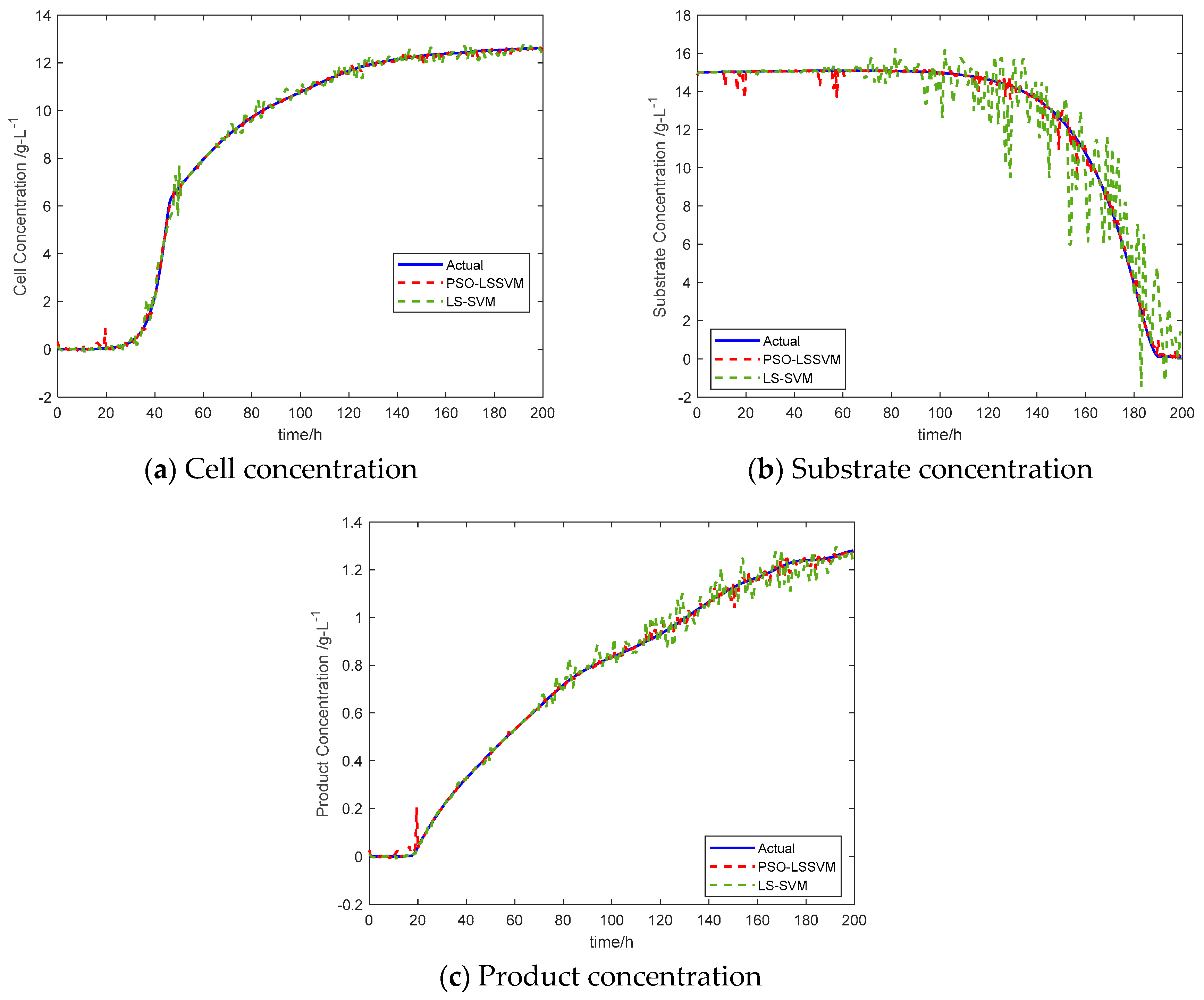
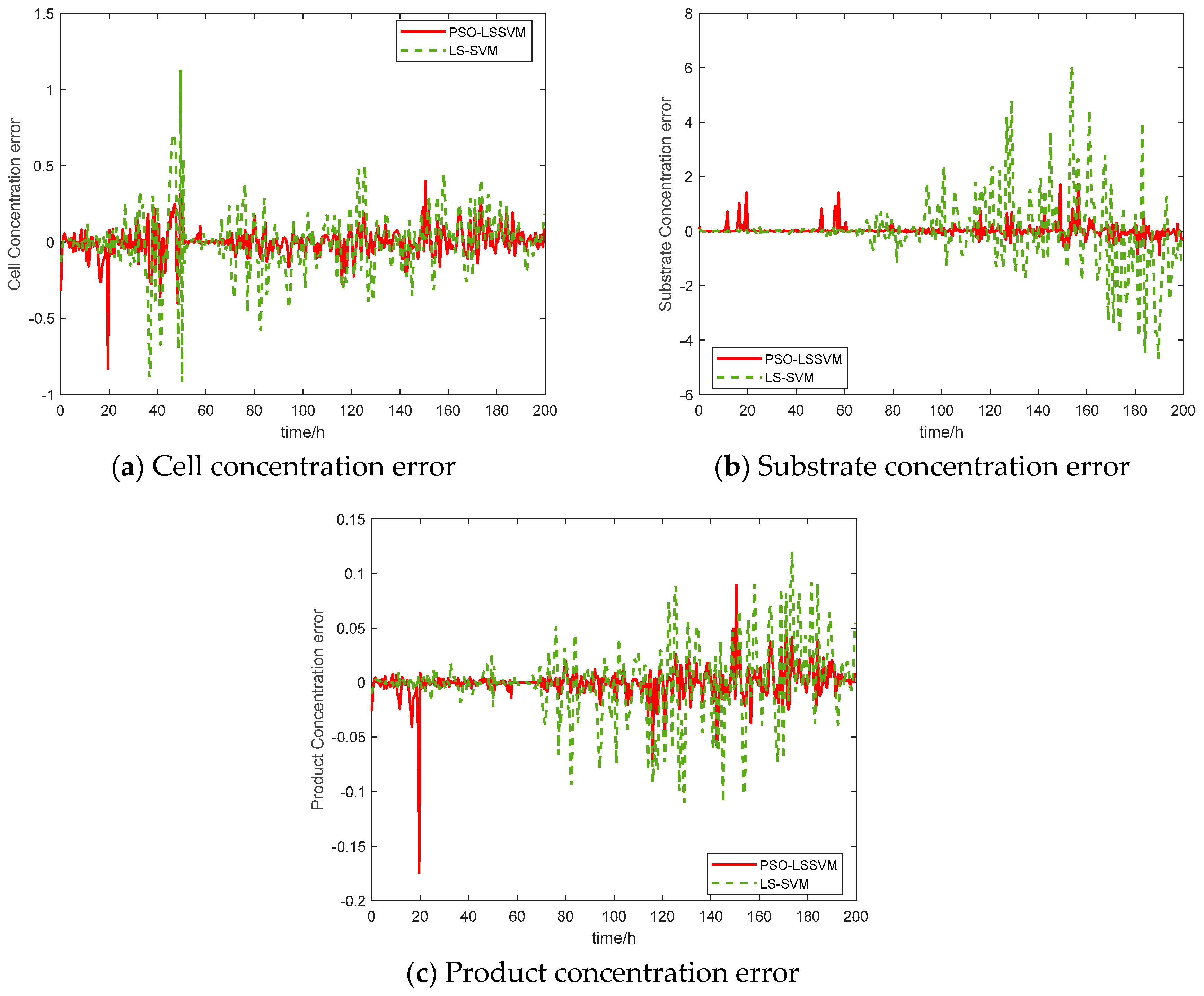
| Key Variables | LS-SVM | PSO-LS-SVM | ||
|---|---|---|---|---|
| RMSE | MAE | RMSE | MAE | |
| X | 0.2114 | 0.139 | 0.1028 | 0.067 |
| S | 1.2761 | 0.741 | 0.2597 | 0.125 |
| P | 0.0339 | 0.022 | 0.0160 | 0.008 |
| Ref | Prediction model | Compared with | RMSE/MSE | MAXE | Best Performance |
|---|---|---|---|---|---|
| [57] | LS-SVM | RBF-NN | - | - | LS-SVM |
| [45] | LS-SVM | NN | - | - | LS-SVM |
| [49] | SVM | BP-NN | - | - | SVM |
| [50] | PSO-LS-SVM | 0.7835 | 0.486 | PSO-LS-SVM | |
| LS-SVM | 0.1032 | 1.493 | |||
| [51] | PSO-SVM | SVM | - | - | PSO-SVM |
| [52] | ABC-MLS-SVM | PID control | - | - | ABC-MLS-SVM |
| [54] | GRA-LS-SVM | 2.518 | 2.641 | GRA-LS-SVM | |
| RBF-NN | 14.273 | 6.271 | |||
| LS-SVM | 3.219 | 2.847 | |||
| GRA-RBFNN | 4.162 | 3.594 | |||
| [56] | IPSO-SVM | PSO | - | - | IPSO-SVM |
| [58] | MLS-SVM Inversion | LS-SVM | - | - | MLS-SVM Inversion |
| Ref | Prediction model | Compared with | RMSE/MSE | MAXE | Best Performance |
|---|---|---|---|---|---|
| [31] | NN-MIV | 27.512 | - | NN-MIV | |
| NN | 37.943 | ||||
| [61] | GPR-NN MIV | 0.0436 | 0.1440 | GPR-NN-MIV | |
| GPR | 0.1082 | 0.4373 | |||
| [23] | RBF-NN | BP | - | - | RBF-NN |
| [62] | PSO-NN | BPNN | - | - | PSO-NN |
| [65] | Novel SS ANN | General SS-ANN | - | - | Novel SS-ANN |
| [66] | GRNN | RBF-NN | - | - | GRNN |
| [67] | KPCA-RBF-NN | PCA | - | - | KPCA-RBF-NN |
| Ref | Prediction Model | Compared with | RMSE/MSE | MAXE | Best Performance |
|---|---|---|---|---|---|
| [43] | FNN Inverse System | PID control | - | - | FNN Inverse sys |
| [89] | GD-FNN | 0.0064 | |||
| RBF-NN | 0.0194 | GD-FNN | |||
| [90] | MNN-KFCM | 0.1963 | - | MNN-MFKC | |
| Single NN | 0.5441 | ||||
| [91] | FLS-SVM | LS-SVM | - | - | FLS-SVM |
| [92] | PSO-FNN | 0.1141 | 0.6151 | PSO-FNN | |
| FNN | 1.3658 | 3.5640 | |||
| [93] | Fuzzy LS-SVM | 0.0097 | - | Fuzzy LS-SVM | |
| LS-SVM | 0.0244 |
| Ref | Prediction Model | Compared with | RMSE/MSE | MAXE | Best Performance |
|---|---|---|---|---|---|
| [96] | GA-SVR | 0.1353 | 0.8872 | GA-SVR | |
| ANN | 0.9217 | 2.3529 | |||
| [97] | GA-SVM | NN | - | - | GA-SVM |
| GA-BPNN | - | - | - | GA-BPNN | |
| [98] | Hybrid GA-ACO | Conventional GA and stand-alone ACO | - | - | Hybrid GA-ACO |
© 2020 by the authors. Licensee MDPI, Basel, Switzerland. This article is an open access article distributed under the terms and conditions of the Creative Commons Attribution (CC BY) license (http://creativecommons.org/licenses/by/4.0/).
Share and Cite
Zhu, X.; Rehman, K.U.; Wang, B.; Shahzad, M. Modern Soft-Sensing Modeling Methods for Fermentation Processes. Sensors 2020, 20, 1771. https://doi.org/10.3390/s20061771
Zhu X, Rehman KU, Wang B, Shahzad M. Modern Soft-Sensing Modeling Methods for Fermentation Processes. Sensors. 2020; 20(6):1771. https://doi.org/10.3390/s20061771
Chicago/Turabian StyleZhu, Xianglin, Khalil Ur Rehman, Bo Wang, and Muhammad Shahzad. 2020. "Modern Soft-Sensing Modeling Methods for Fermentation Processes" Sensors 20, no. 6: 1771. https://doi.org/10.3390/s20061771
APA StyleZhu, X., Rehman, K. U., Wang, B., & Shahzad, M. (2020). Modern Soft-Sensing Modeling Methods for Fermentation Processes. Sensors, 20(6), 1771. https://doi.org/10.3390/s20061771