A New Fault Feature Extraction Method for Rotating Machinery Based on Multiple Sensors


Abstract
:1. Introduction
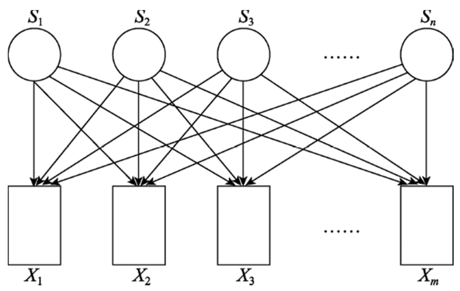
2. Multi-Sensor Test System Model
3. Median Filter
4. Independent Component Analysis Based on JADE
4.1. Hybrid Matrix A Estimation Based on the Fourth-Order Cumulant
4.2. Signal Whitening
4.3. Joint Approximate Diagonalization
5. Blind Source Separation of Multi-Fault Vibration Signals Based on MF-JADE
5.1. Basic Steps
5.2. Evaluation Index of Separation Effect
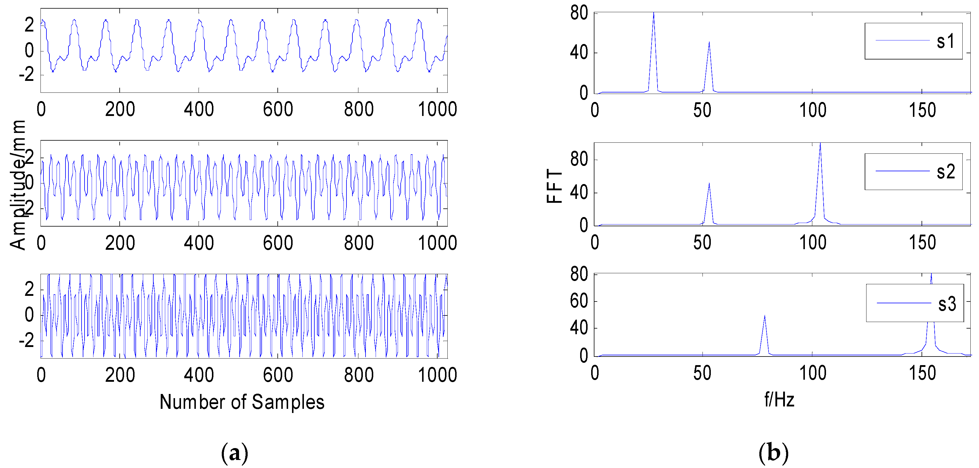
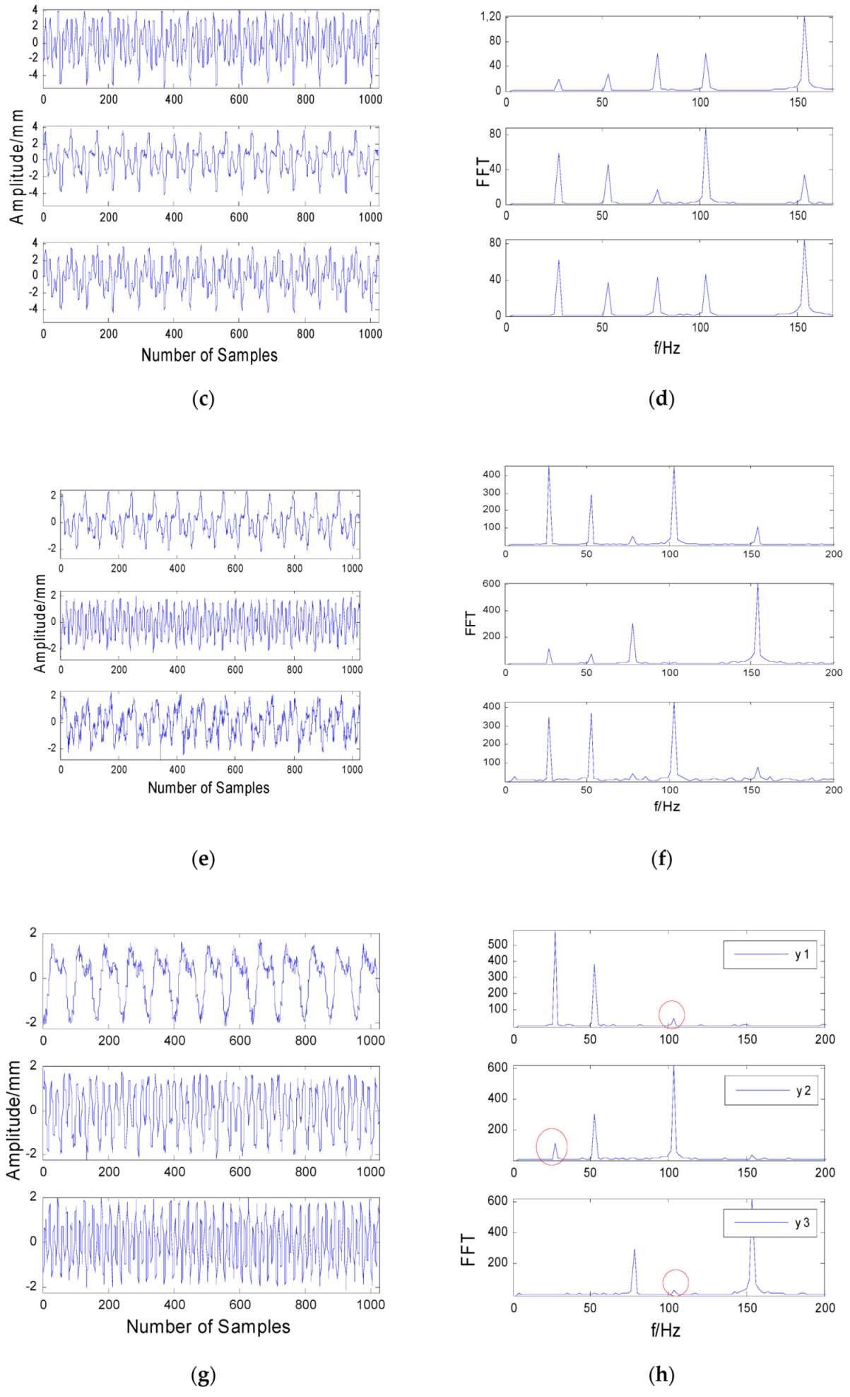
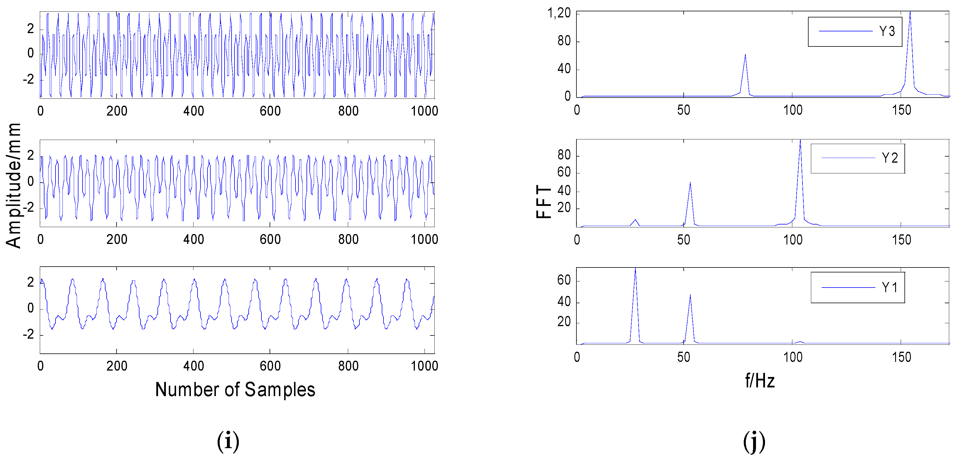
6. Simulations
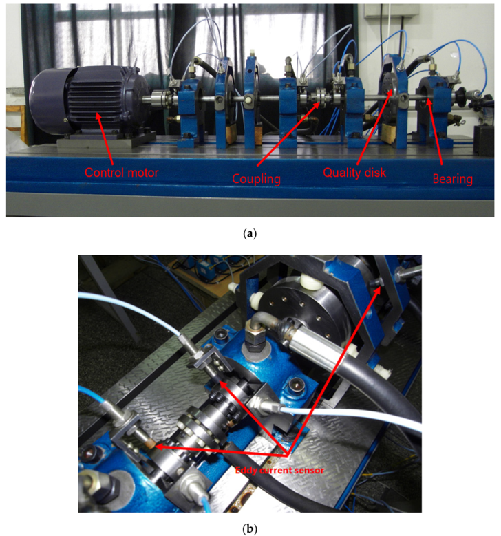
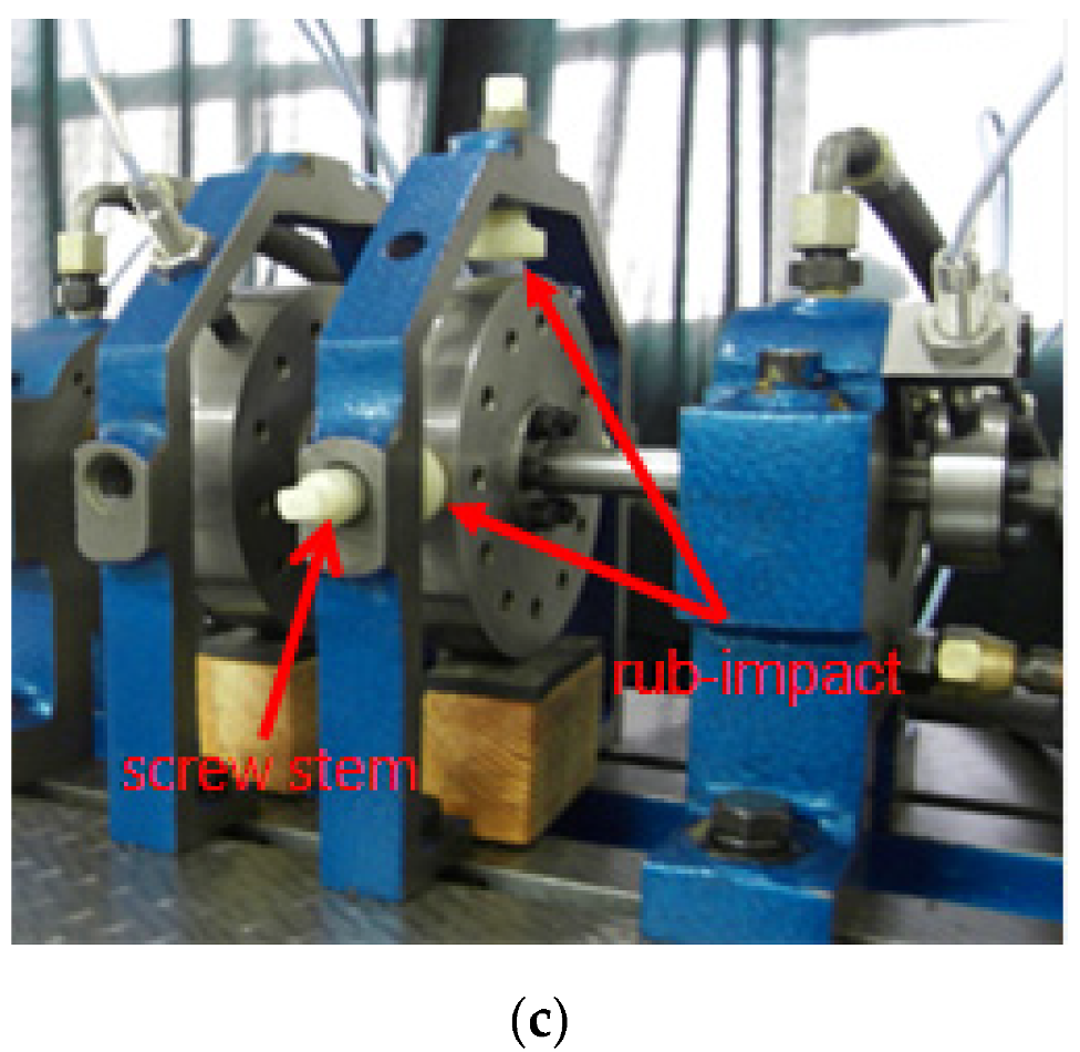
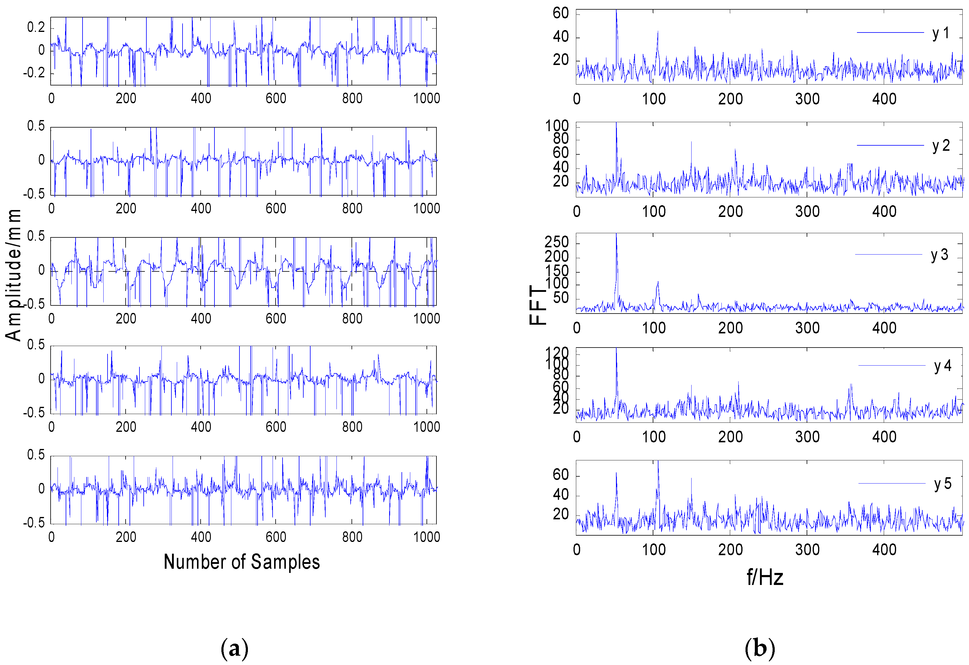
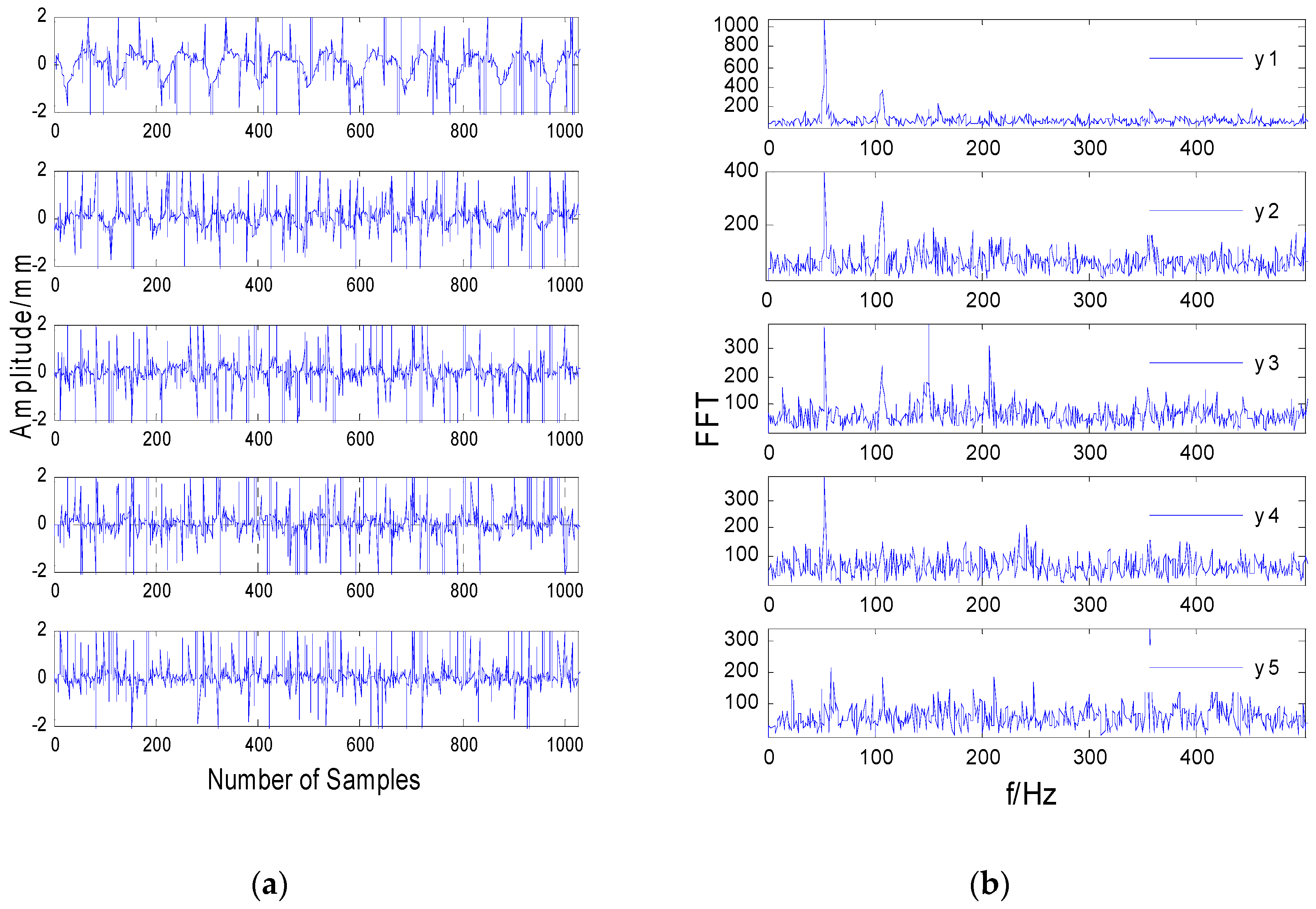
7. Experiments
8. Conclusions
- Blind separation of the observation signal with strong impulse noise was carried out directly, and the error of the separation result was large, where even an incorrect result could be obtained.
- The median filtering method can effectively remove the impulse noise signal without losing the useful components of the original signal, improve the signal-to-noise ratio, and provide precondition for the accurate realization of blind separation.
- For the measured signal, although the independence assumption of blind source separation is not strictly true, the MF-JADE algorithm is still effective in the actual vibration signal separation.
- The combination of a median filtering method and a blind source separation algorithm provides a new method for the separation of aliased signals in strong impulse noise environments.
Author Contributions
Funding
Conflicts of Interest
References
- Fu, W.; Tan, J.; Zhang, X.; Chen, T.; Wang, K. Blind Parameter Identification of MAR Model and Mutation Hybrid. GWO-SCA Optimized SVM for Fault Diagnosis of Rotating Machinery. Complexity 2019, 2019, 3264969. [Google Scholar] [CrossRef]
- Glowacz, A. Fault diagnosis of single-phase induction motor based on acoustic signals. Mech. Syst. Signal Process. 2019, 117, 65–80. [Google Scholar] [CrossRef]
- Xia, M.; Li, T.; Xu, L.; Liu, L.; De, W. Fault Diagnosis for Rotating Machinery Using Multiple Sensors and Convolutional Neural Networks. IEEE-Asme Trans. Mechatron. 2018, 23, 101–110. [Google Scholar] [CrossRef]
- Jiang, X.; Wang, J.; Shi, J.; Shen, C.; Huang, W.; Zhu, Z. A coarse-to-fine decomposing strategy of VMD for extraction of weak repetitive transients in fault diagnosis of rotating machines. Mech. Syst. Signal Process. 2019, 116, 668–692. [Google Scholar] [CrossRef]
- Song, L.; Wang, H.; Chen, P. Vibration-Based Intelligent Fault Diagnosis for Roller Bearings in Low-Speed Rotating Machinery. IEEE Trans. Instrum. Meas. 2018, 67, 1887–1899. [Google Scholar] [CrossRef]
- Shao, H.; Jiang, H.; Zhao, H.; Wang, F. A novel deep autoencoder feature learning method for rotating machinery fault diagnosis. Mech. Syst. Signal Process. 2017, 95, 187–204. [Google Scholar] [CrossRef]
- Shao, H.; Jiang, H.; Zhao, H.; Wang, F. An enhancement deep feature fusion method for rotating machinery fault diagnosis. Knowl. Based Syst. 2017, 119, 200–220. [Google Scholar] [CrossRef]
- Rostaghi, M.; Ashory, M.R.; Azami, H. Application of dispersion entropy to status characterization of rotary machines. J. Sound Vib. 2019, 438, 291–308. [Google Scholar] [CrossRef]
- Lun, D.P.K.; Chan, Y.-H. Robust Single-Shot Fringe Projection Profilometry Based on Morphological Component Analysis. IEEE Trans. Image Process. 2018, 27, 5393–5405. [Google Scholar]
- Conci, A.; Rodrigues, E.O.; Liatsis, P. Morphological classifiers. Pattern Recognit. 2018, 84, 82–96. [Google Scholar]
- Huang, W.; Liu, J. Robust Seismic Image Interpolation with Mathematical Morphological Constraint. IEEE Trans. Image Process. 2020, 29, 819–829. [Google Scholar] [CrossRef] [PubMed]
- Legaz-Aparicio, A.-G.; Verdu-Monedero, R.; Angulo, J. Adaptive morphological filters based on a multiple orientation vector field dependent on image local features. J. Comput. Appl. Math. 2018, 330, 965–981. [Google Scholar] [CrossRef] [Green Version]
- Lin, H.; Hu, Y.; Chen, S.; Yao, J.; Zhang, L. Fine-grained classification of cervical cells using morphological and appearance based convolutional neural networks. IEEE Access 2019, 7, 71541–71549. [Google Scholar] [CrossRef]
- Luo, B.; Zhang, L. Robust autodual morphological profiles for the classification of high-resolution satellite images. IEEE Trans. Geosci. Remote Sens. 2014, 52, 1451–1462. [Google Scholar] [CrossRef]
- Lv, Z.; Zhang, P.; Benediktsson, J.; Shi, W. Morphological profiles based on differently shaped structuring elements for classi fication of images with very high spatial resolution. IEEE J. Sel. Top. Appl. Earth Obs. Remote Sens. 2014, 7, 4644–4652. [Google Scholar] [CrossRef]
- Ma, W.; Wan, Y.; Li, J.; Zhu, S.; Wang, M. An automatic morphological attribute building extraction approach for satellite high spatial resolution imagery. Remote Sens. 2019, 11, 337. [Google Scholar] [CrossRef] [Green Version]
- Naderi, H.; Fathianpour, N.; Tabaei, M. MORPHSIM: A new multiple-point pattern-based unconditional simulation algorithm using morphological image processing tools. J. Pet. Sci. Eng. 2019, 173, 1417–1437. [Google Scholar] [CrossRef]
- Nair, V.; Ram, P.G.K.; Sundararaman, S. Shadow detection and removal from images using machine learning and morphological operations. J. Eng. 2019, 2019, 11–18. [Google Scholar] [CrossRef]
- Ritchey, T. General morphological analysis as a basic scientific modelling method. Technol. Forecast. Soc. Chang. 2018, 126, 81–91. [Google Scholar] [CrossRef]
- Salazar-Colores, S.; Cabal-Yepez, E.; Ramos-Arreguin, J.; Botella, G.; Ledesma-Carrillo, L.; Ledesma, S. A Fast Image Dehazing Algorithm Using Morphological Reconstruction. IEEE Trans. Image Process. 2019, 28, 2357–2366. [Google Scholar] [CrossRef]
- Tong, W.; Li, H.; Chen, G. Blob detection based on soft morphological filter. IEICE Trans. Inf. Syst. 2020, E103D, 152–162. [Google Scholar] [CrossRef] [Green Version]
- Wang, Z. A new clustering method based on morphological operations. Expert Syst. Appl. 2020, 145, 113102. [Google Scholar] [CrossRef] [Green Version]
- Xue, B.; Hong, H.; Zhou, S.; Chen, G.; Li, Y.; Wang, Z.; Zhu, X. Morphological Filtering Enhanced Empirical Wavelet Transform for Mode Decomposition. IEEE Access 2019, 7, 14283–14293. [Google Scholar] [CrossRef]
- Yan, X.; Liu, Y.; Jia, M. A feature selection framework-based multiscale morphological analysis algorithm for fault diagnosis of rolling element bearing. IEEE Access 2019, 7, 123436–123452. [Google Scholar] [CrossRef]
- Zhang, B.; Hu, Q.; Wei, L.; Li, S. Improved morphological filtering algorithm of interferograms. Xi Tong Gong Cheng Yu Dian Zi Ji Shu/Syst. Eng. Electron. 2018, 40, 2230–2236. [Google Scholar]
- Zhang, X.; Tang, C.; Zhou, R.; Lei, W. Adaptive Morphological Filtering Algorithm with Applications in Bearing Fault Diagnosis. Hsi-Chiao Tung Ta Hsueh/J. Xi’an Jiaotong Univ. 2018, 52, 1–8, 37. [Google Scholar]
- Benko, G.; Juhasz, Z. GPU implementation of the FastICA algorithm. In Proceedings of the 42nd International Convention on Information and Communication Technology, Electronics and Microelectronics, MIPRO 2019, Opatija, Croatia, 20–24 May 2019; Institute of Electrical and Electronics Engineers Inc.: Opatija, Croatia, 2019. [Google Scholar]
- Chen, L.; Gan, S.; Zhang, L.; Wang, G. Nonlinear blind source separation algorithm based on spline interpolation and artificial bee colony optimization. Tongxin Xuebao/J. Commun. 2017, 38, 36–46. [Google Scholar]
- Li, C.; De Oliveira, J.V.; Cerrada, M.; Cabrera, D.; Sanchez, R.; Zurita, G. A Systematic Review of Fuzzy Formalisms for Bearing Fault Diagnosis. IEEE Trans. Fuzzy Syst. 2019, 27, 1362–1382. [Google Scholar]
- Zhang, H.; Ma, J.; Jing, J.; Li, P. Fabric defect detection method based on improved fast weighted median filtering and K-means. J. Text. Res. 2019, 40, 50–56. [Google Scholar]
- Lu, S.; He, Q.; Wang, J. A review of stochastic resonance in rotating machine fault detection. Mech. Syst. Signal Process. 2019, 116, 230–260. [Google Scholar] [CrossRef]
- Aldhahab, A.; Mikhael, W.B. Face Recognition Employing DMWT Followed by FastICA. Circuits Syst. Signal Process. 2018, 37, 2045–2073. [Google Scholar] [CrossRef]
- Fantinato, D.; Duarte, L.; Deville, Y.; Attux, R.; Jutten, C.; Neves, A. A second-order statistics method for blind source separation in post-nonlinear mixtures. Signal Process. 2019, 155, 63–72. [Google Scholar] [CrossRef] [Green Version]
- Huang, J.; Sun, J. Sampling Adaptive Learning Algorithm for Mobile Blind Source Separation. Wirel. Commun. Mob. Comput. 2018, 2018, 5048419. [Google Scholar] [CrossRef] [Green Version]
- Li, Y.; Nie, W.; Ye, F.; Wang, Q. A complex mixing matrix estimation algorithm in under-determined blind source separation problems. Signal Image Video Process. 2017, 11, 301–308. [Google Scholar] [CrossRef]
- Zhou, Y.; Li, S.; Zhang, D.; Chen, Y. Seismic noise attenuation using an online subspace tracking algorithm. Geophys. J. Int. 2018, 212, 1072–1097. [Google Scholar] [CrossRef] [Green Version]
- Yang, J.; Zhang, Y.; Yin, W. An Efficient Tvl1 Algorithm for Deblurring Multichannel Images Corrupted by Impulsive Noise. Siam J. Sci. Comput. 2009, 31, 2842–2865. [Google Scholar] [CrossRef]
- Babaee, M.; Tung, D.D.; Rigoll, G. A deep convolutional neural network for video sequence background subtraction. Pattern Recognit. 2018, 76, 635–649. [Google Scholar] [CrossRef]
- Qin, Z.; Yi, Y.-Q.; Lin, Y.-P. Robust watermark based on JADE algorithm. Tien Tzu Hsueh Pao/Acta Electron. Sin. 2008, 36, 1149–1153. [Google Scholar]

| Algorithm | VQM/dB | PI | ||
|---|---|---|---|---|
| Fast-ICA | 0.455 | 1.612 | ||
| 0.523 | −2.765 | 3.415 | ||
| 0.632 | −3.316 | |||
| JADE | 0.579 | −3.422 | ||
| 0.814 | −8.563 | 3.413 | ||
| 0.611 | −2.013 | |||
| MF-FastICA | 0.915 | −14.213 | ||
| 0.921 | −13.612 | 0.965 | ||
| 0.936 | −15.518 | |||
| MF-JADE | 0.998 | −23.612 | ||
| 0.986 | −20.965 | 0.311 | ||
| 0.997 | −22.953 |
© 2020 by the authors. Licensee MDPI, Basel, Switzerland. This article is an open access article distributed under the terms and conditions of the Creative Commons Attribution (CC BY) license (http://creativecommons.org/licenses/by/4.0/).
Share and Cite
Miao, F.; Zhao, R.; Wang, X.; Jia, L. A New Fault Feature Extraction Method for Rotating Machinery Based on Multiple Sensors. Sensors 2020, 20, 1713. https://doi.org/10.3390/s20061713
Miao F, Zhao R, Wang X, Jia L. A New Fault Feature Extraction Method for Rotating Machinery Based on Multiple Sensors. Sensors. 2020; 20(6):1713. https://doi.org/10.3390/s20061713
Chicago/Turabian StyleMiao, Feng, Rongzhen Zhao, Xianli Wang, and Leilei Jia. 2020. "A New Fault Feature Extraction Method for Rotating Machinery Based on Multiple Sensors" Sensors 20, no. 6: 1713. https://doi.org/10.3390/s20061713
APA StyleMiao, F., Zhao, R., Wang, X., & Jia, L. (2020). A New Fault Feature Extraction Method for Rotating Machinery Based on Multiple Sensors. Sensors, 20(6), 1713. https://doi.org/10.3390/s20061713