An Improved LDA-Based ELM Classification for Intrusion Detection Algorithm in IoT Application


Abstract
:1. Introduction
- (1)
- For IoT intrusion detection, we use the similarity measure function of high-dimensional data space as the weight to improve the between-class scatter matrix, and then combine it with LDA to obtain the optimal transformation matrix to achieve the dimensionality reduction of the data. The addition of the similarity measure function of high-dimensional data space gives the data better spatial separation, thereby improving the dimensionality reduction performance.
- (2)
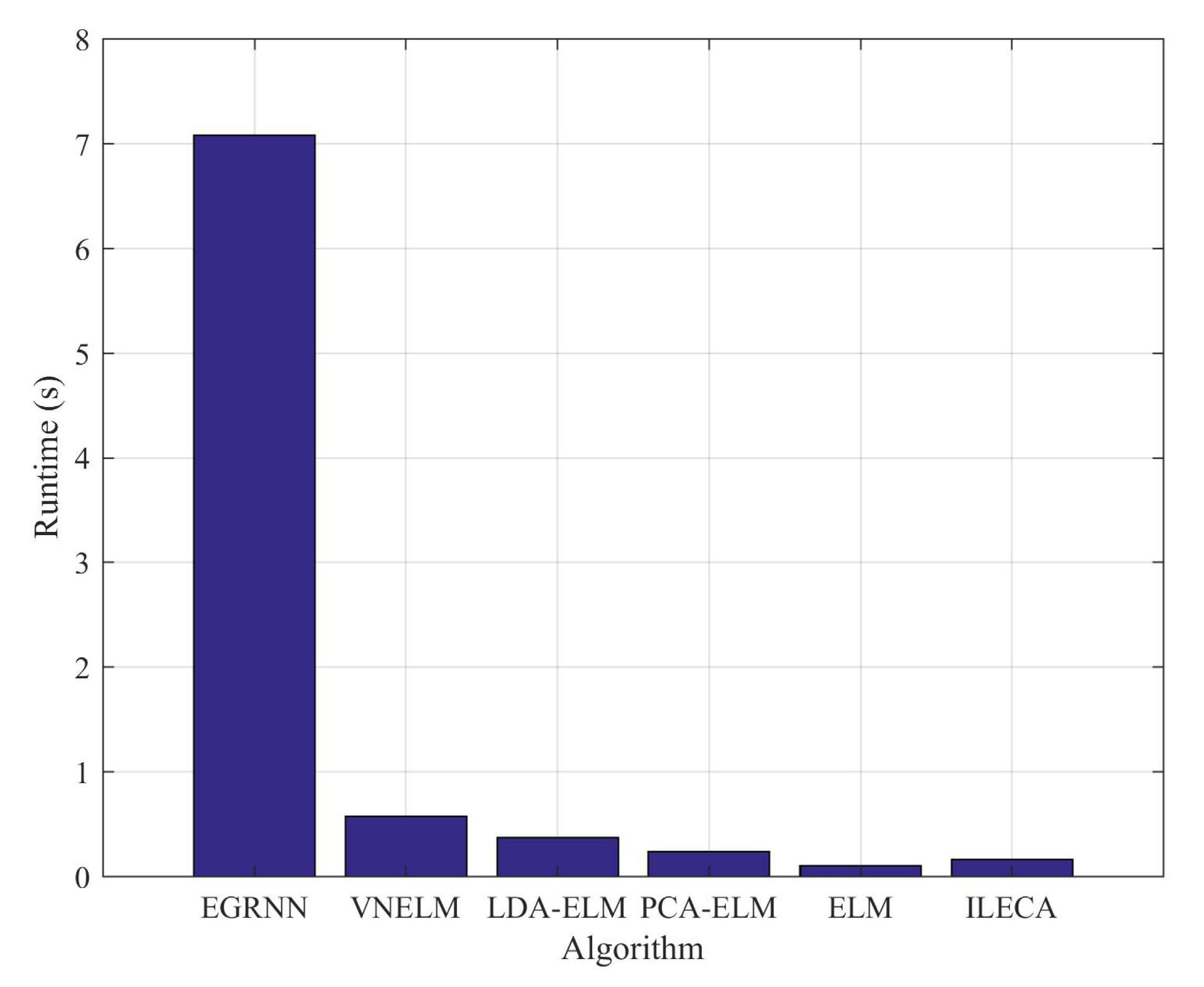
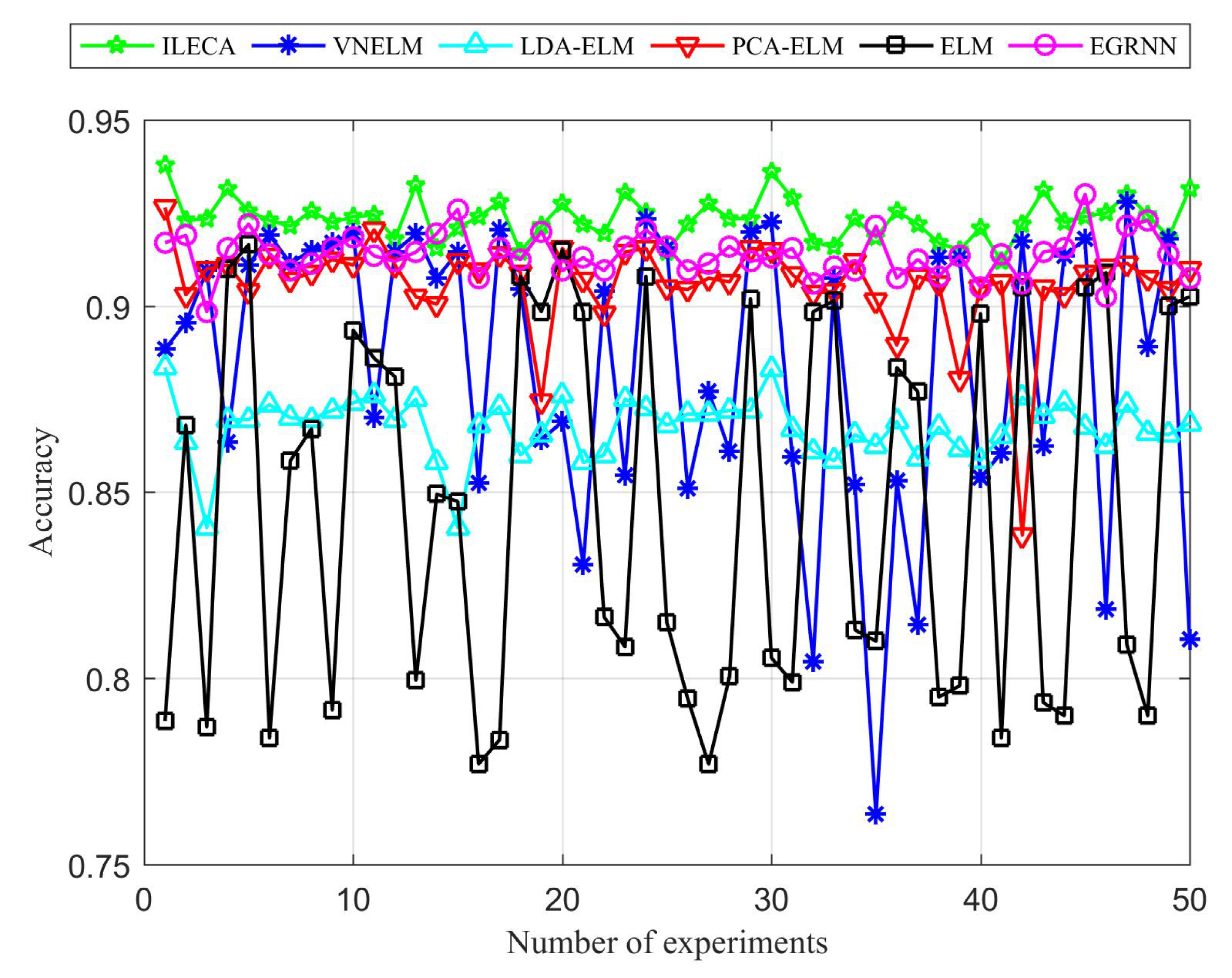
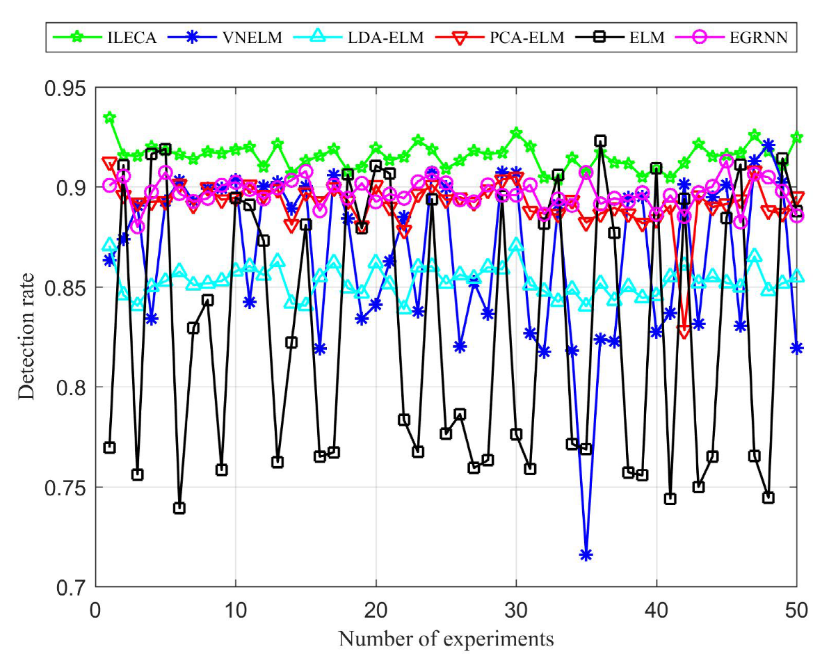
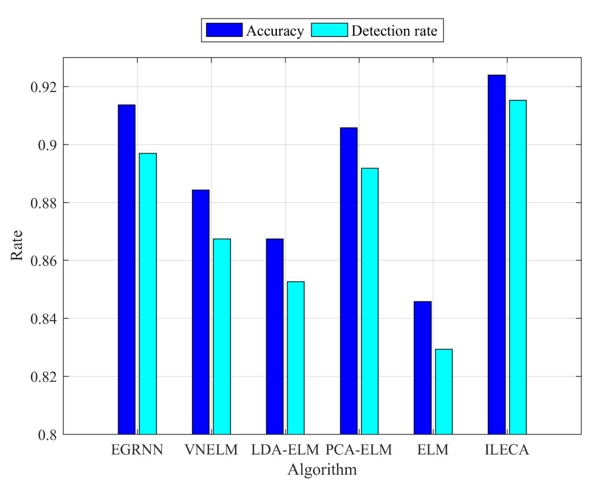
- We use the ELM classification to classify and detect the data after dimension reduction. ELM classification indeed helps speed up the overall learning rate of the algorithm as well as strengthening the capabilities of generalization. After evaluation tests using NSL-KDD, the accuracy and detection rate of our algorithm are, respectively, up to 92.35% and 91.53%, but its runtime is only 0.1632 s, of which the overall performance is better than the other five typical algorithms.
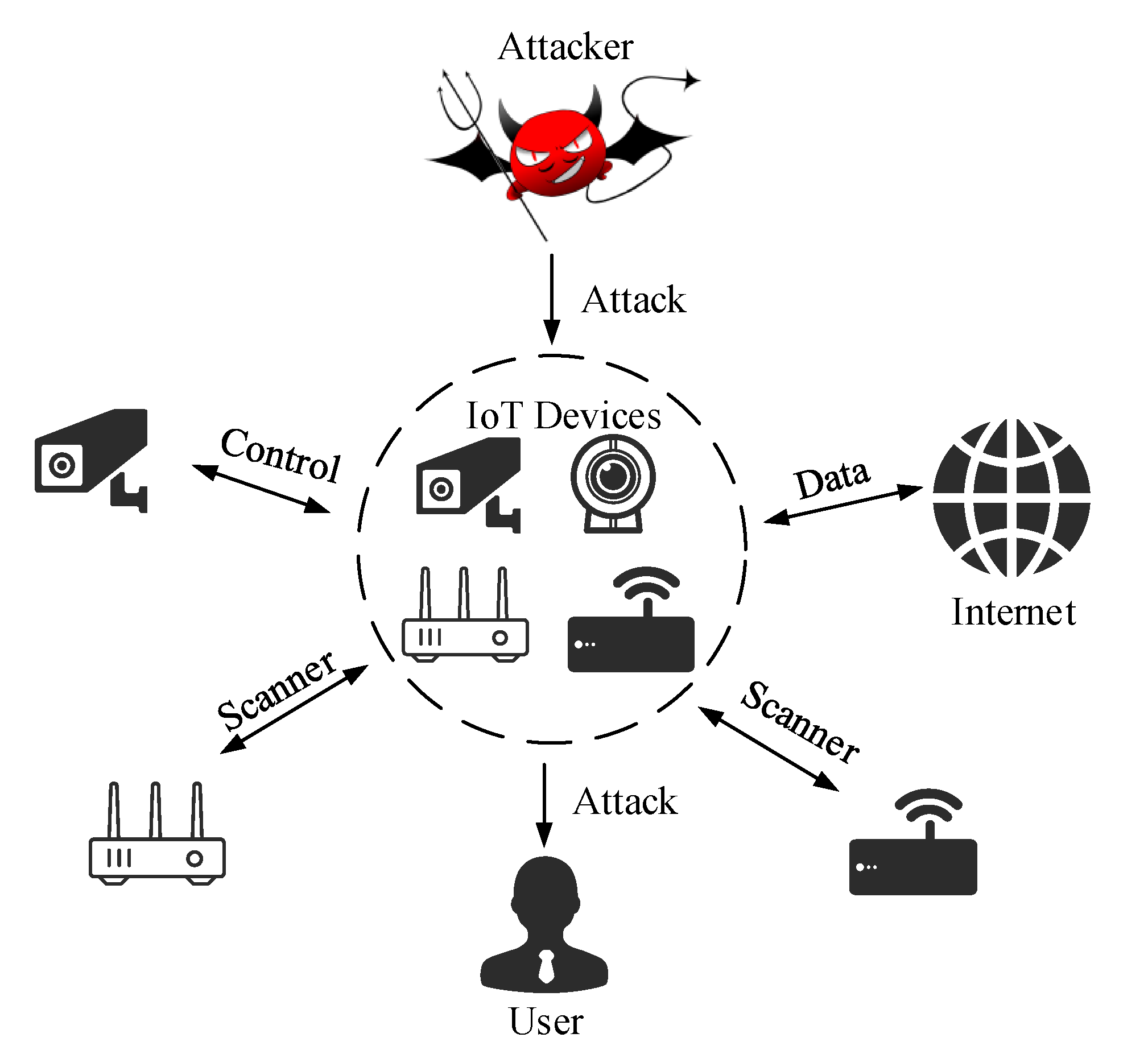
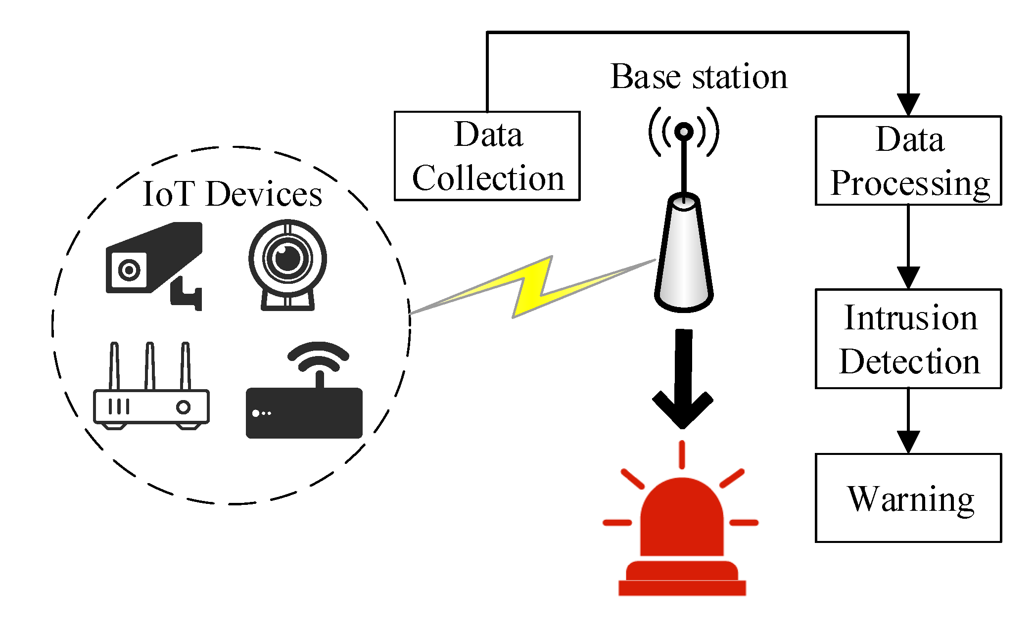
2. Intrusion Detection Model
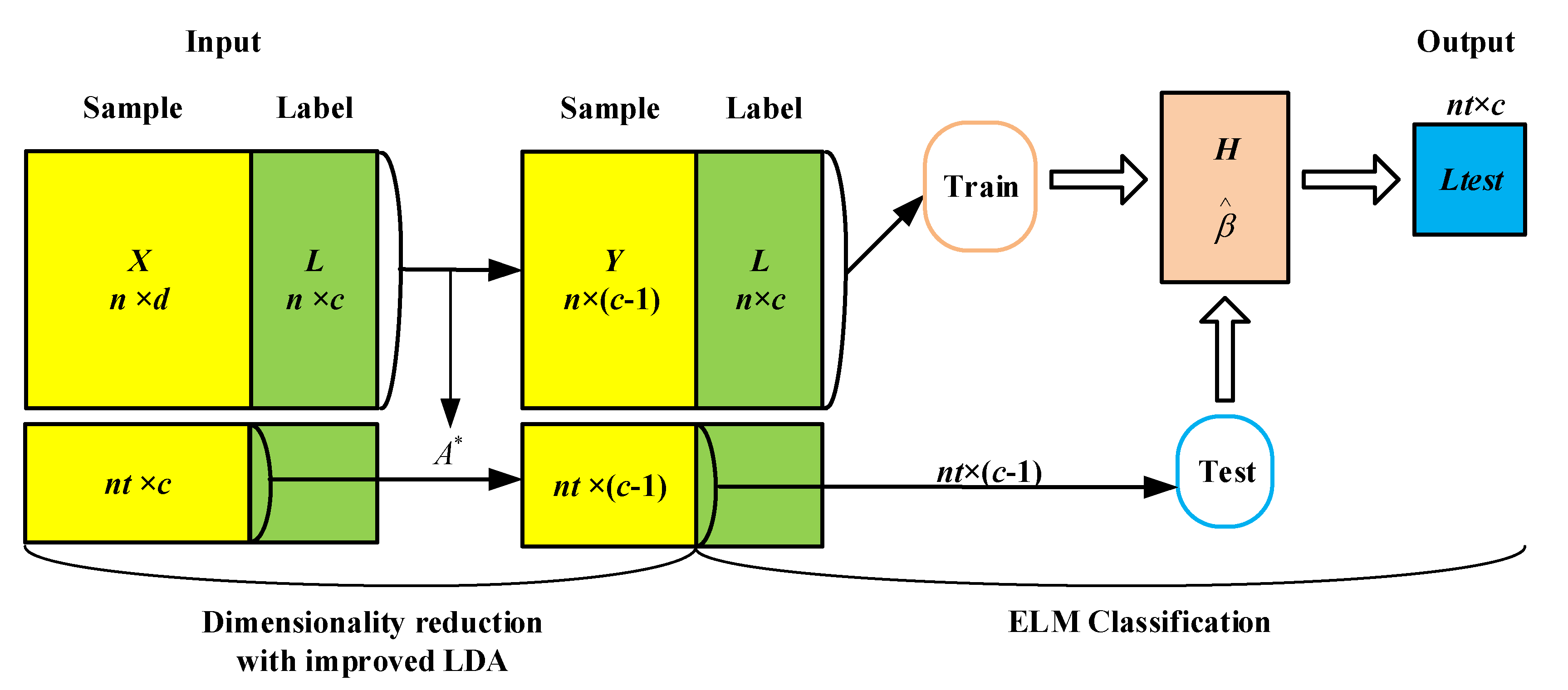
3. The Proposed ILECA
3.1. The Correlated Variables
3.2. Data Preprocessing
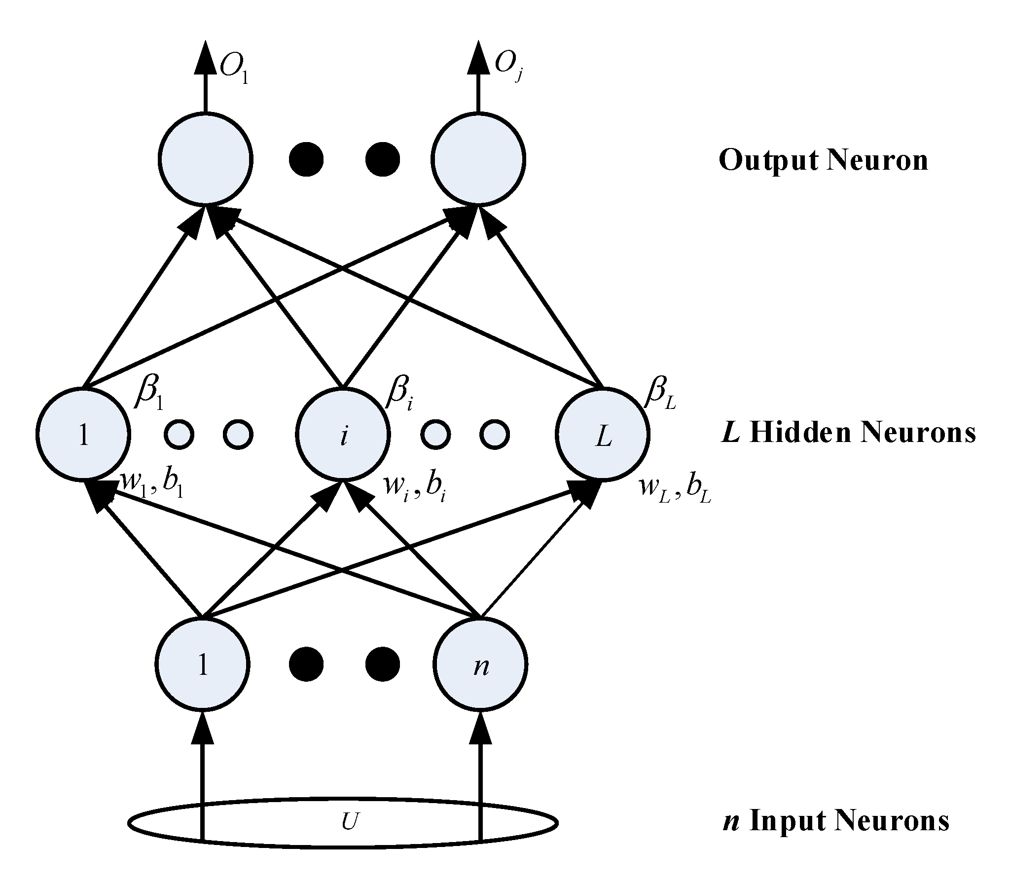
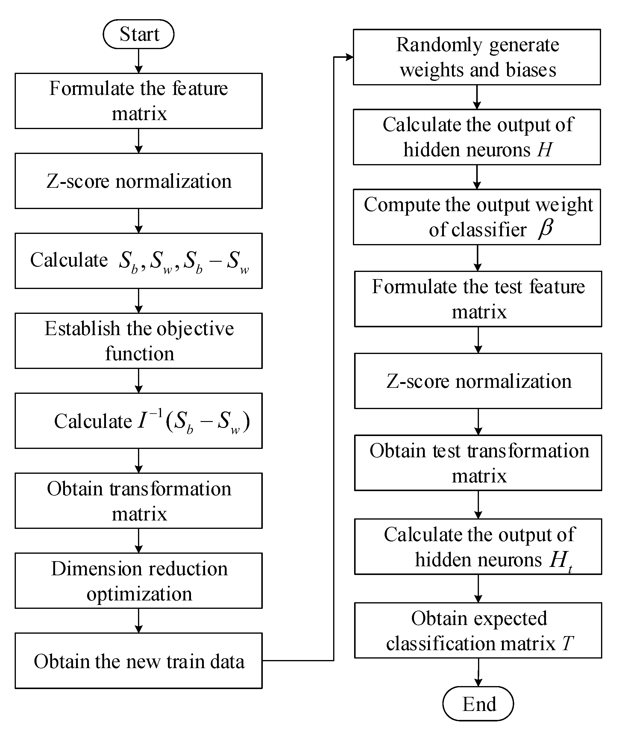
3.3. The Proposed Algorithm
- Step 1: randomly generate the input weight and the offset of the hidden layer node .
- Step 2: calculate the hidden layer output matrix H according to Equation (13).
- Step 3: calculate the optimal output weight according to Equation (14).
| Algorithm 1: ILECA |
| Input: train set , test set Output: expected classification matrix T
|
- Step 1: Perform Z-score normalization on the train samples according to Equation (1).
- Step 3: Establish the objective function according to Equation (7), calculate , and decompose the characteristic problem to obtain the eigenvalues and eigenvectors. Take the eigenvectors corresponding to the first m largest eigenvalues as the transformation matrix , .
- Step 4: Calculate according to Equation (8), and obtain the new train data .
- Step 5: Generate and randomly, and set the number of hidden neurons L.
- Step 6: Calculate the output of hidden neurons H according to the Equation (13).
- Step 7: Calculate the output weight of classifier according to the Equation (14).
- Step 8: Calculate .
- Step 9: Calculate the output of hidden neurons for test data according the to Equation (13).
- Step 10: Calculate the output for test data by Equation (12) with and .
4. Performance Evaluation
4.1. Experimental Set-Up
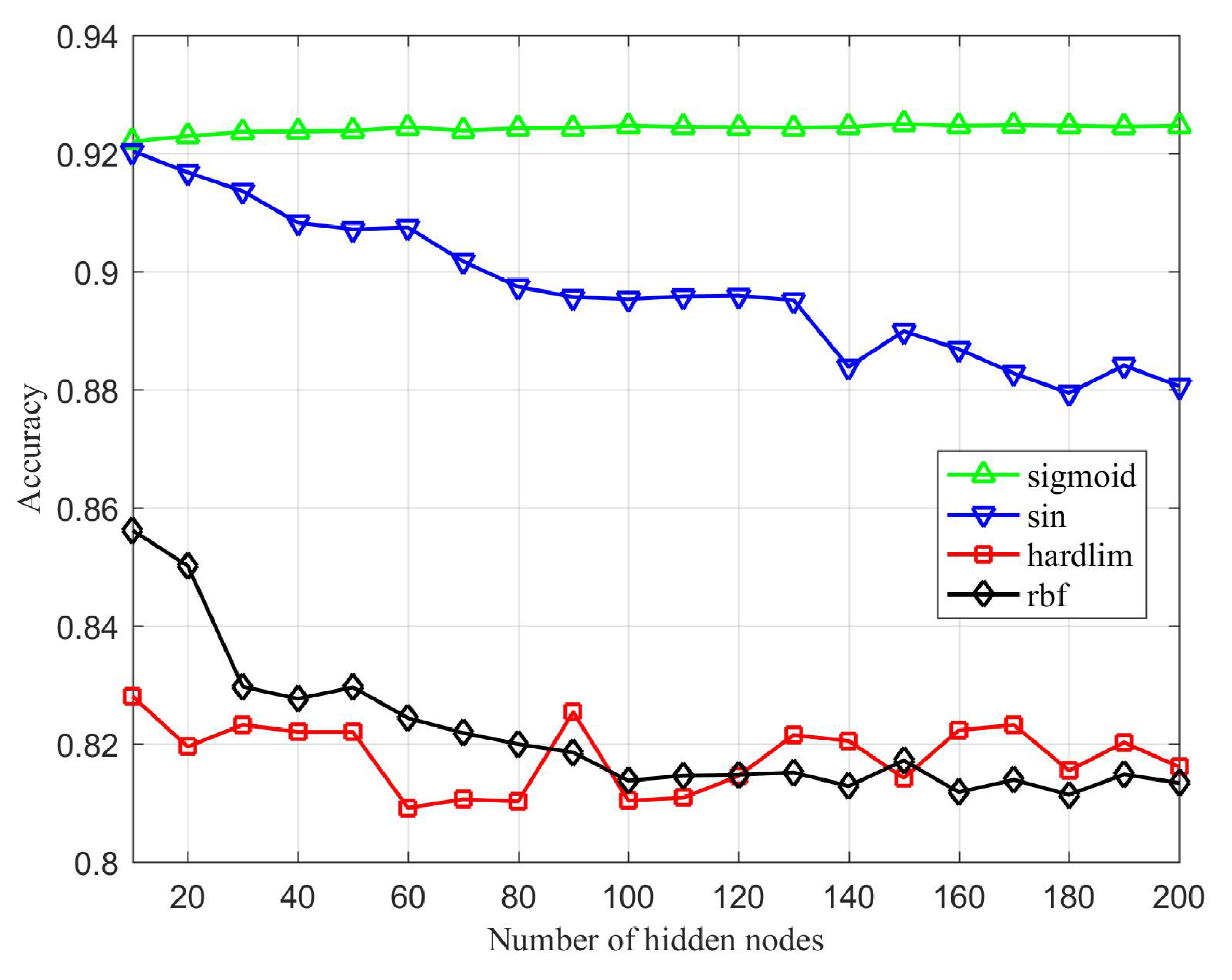
- Accuracy: The proportion of samples predicted to be correct.
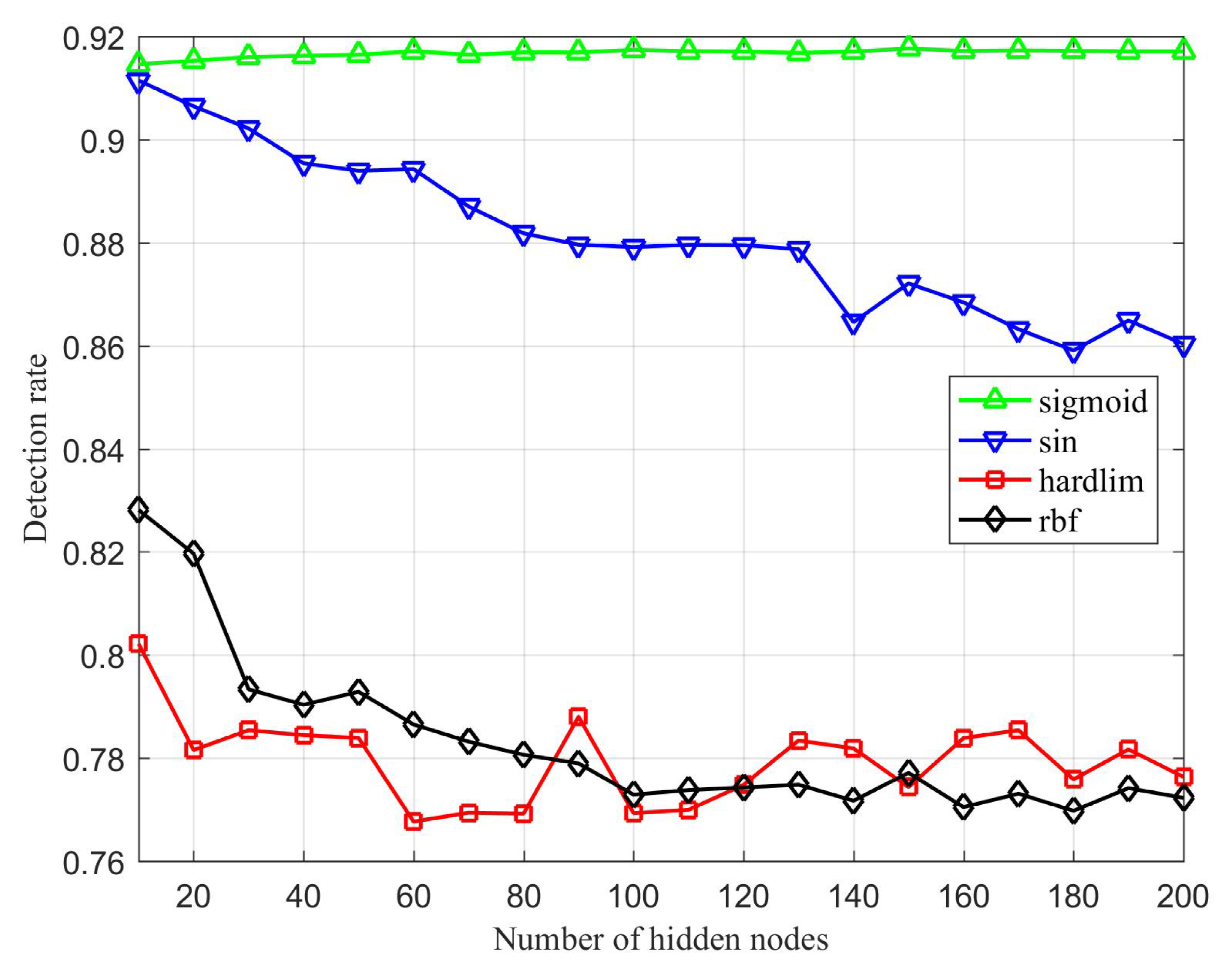
- Detection rate: The proportion of the number of attack samples that are correctly detected to the total number of attack samples.
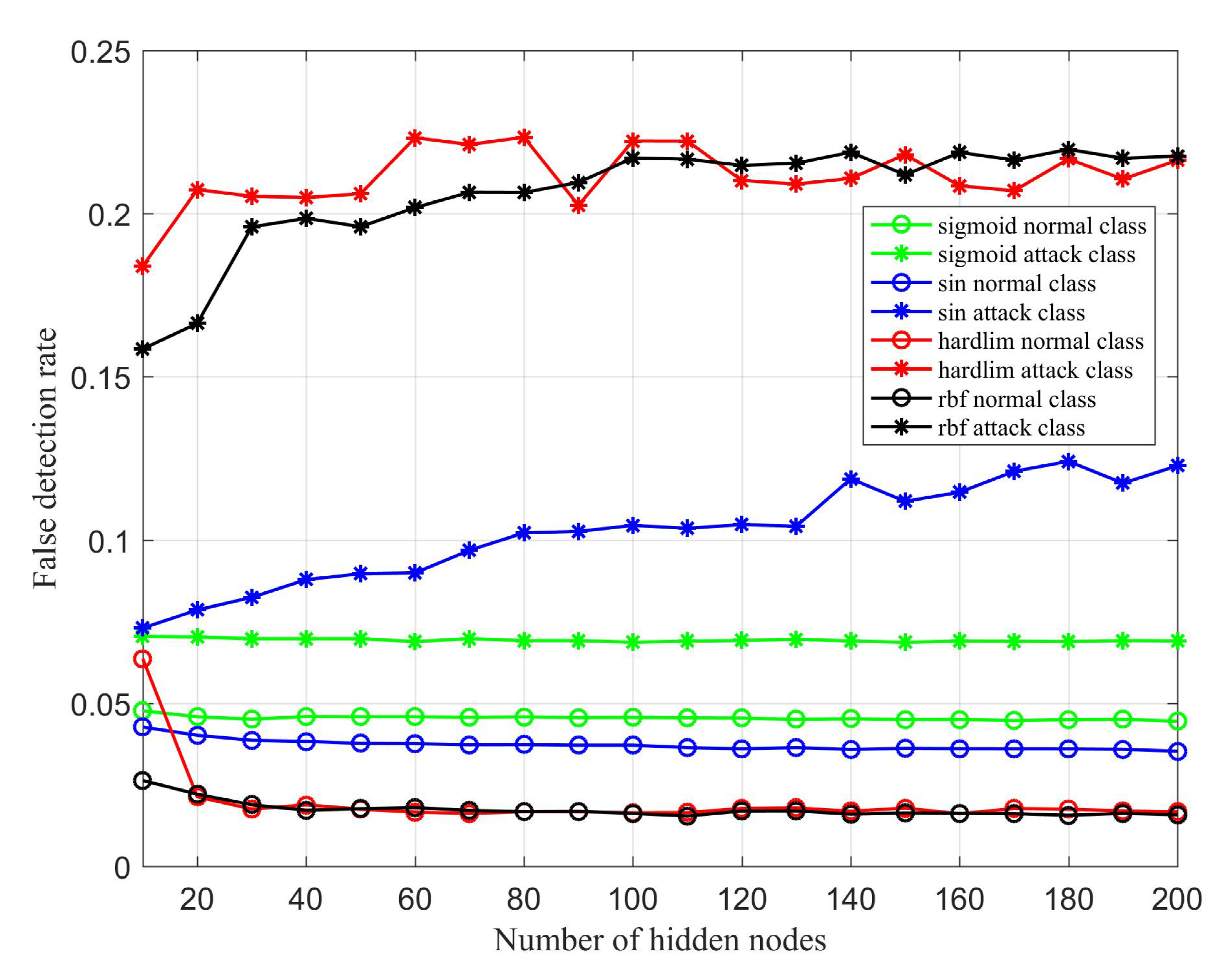
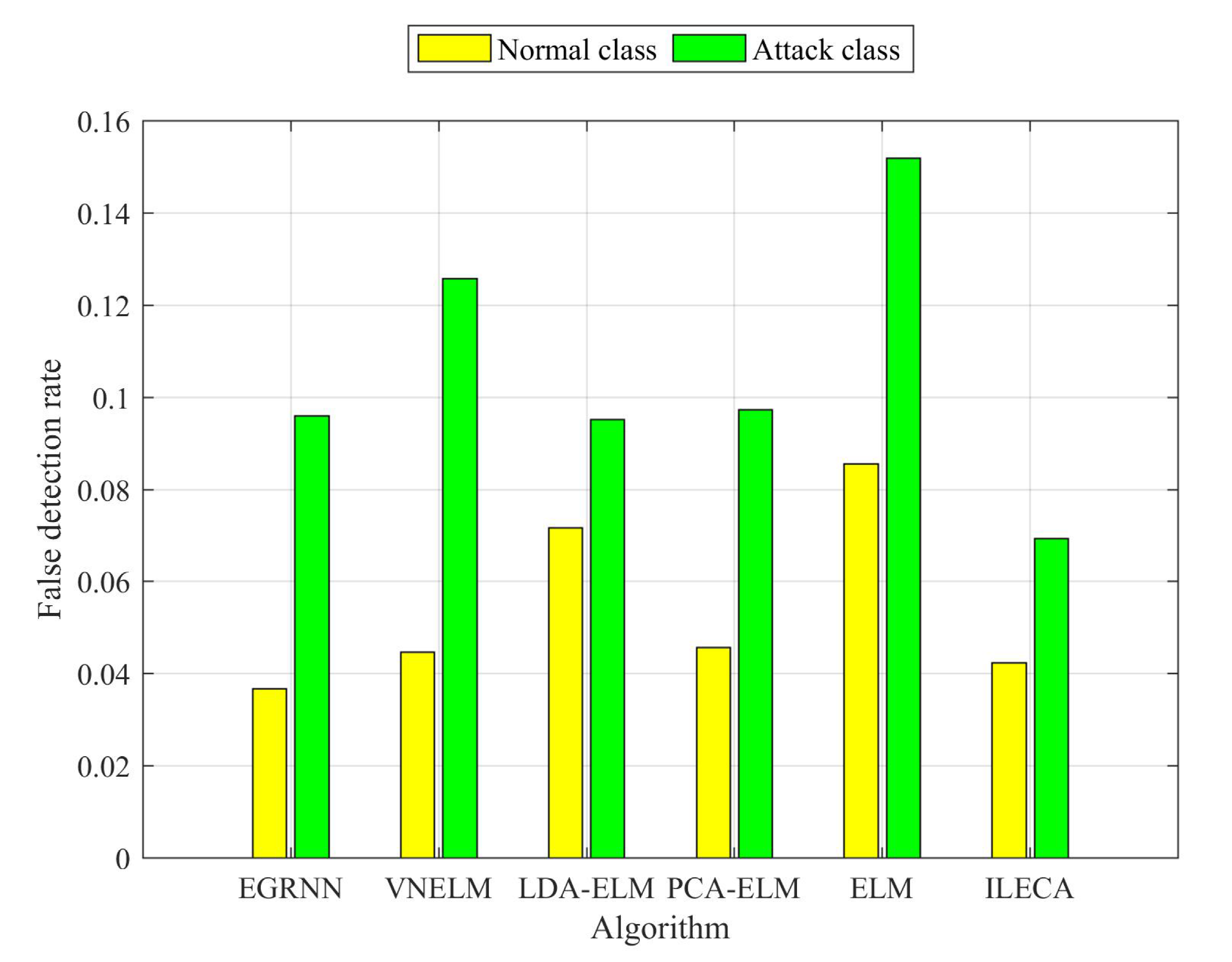
- False detection rate of normal class: The proportion of the normal class samples that are falsely detected as attack classes to the total number of normal class samples.
- False detection rate of attack class: The proportion of the attack class samples that are falsely detected as normal classes to the total number of attack class samples.
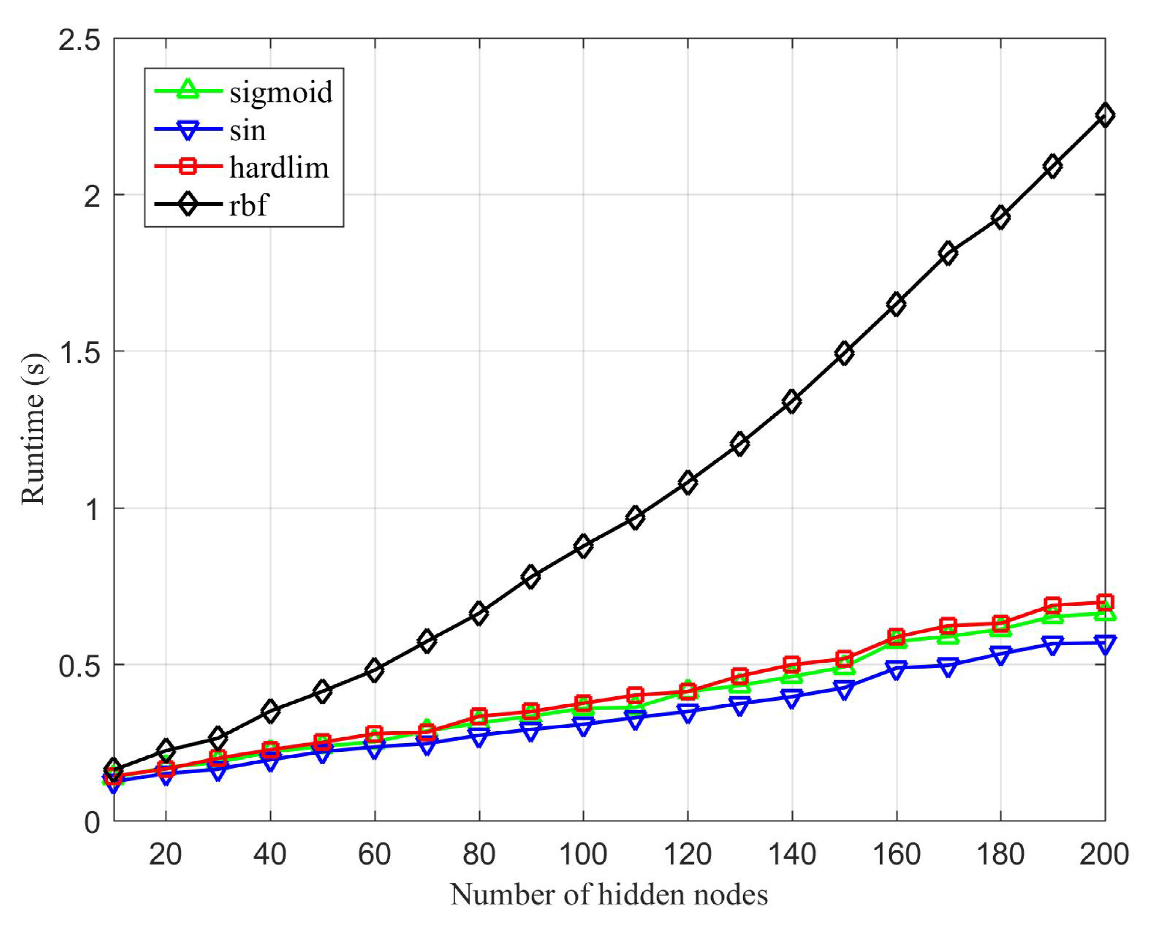
4.2. Meta-Parameter Analysis
4.3. Results and Discussion
5. Conclusion and Future Work
Author Contributions
Funding
Acknowledgments
Conflicts of Interest
References
- Olasupo, T.O. Wireless communication modeling for the deployment of tiny IoT devices in rocky and mountainous environments. IEEE Sens. Lett. 2019, 3, 1–4. [Google Scholar] [CrossRef]
- Roy, S.K.; Misra, S.; Raghuwanshi, N.S. SensPnP: Seamless integration of heterogeneous sensors with IoT devices. IEEE Trans. Consum. Electron. 2019, 65, 205–214. [Google Scholar] [CrossRef]
- Yang, Y.; Zheng, X.; Guo, W.; Liu, X.; Victor, C. Privacy-preserving smart IoT-based healthcare big data storage and self-adaptive access control system. Inf. Sci. 2019, 479, 567–592. [Google Scholar] [CrossRef]
- Meneghello, F.; Calore, M.; Zucchetto, D.; Polese, M.; Zanella, A. IoT: Internet of threats? A survey of practical security vulnerabilities in real iot devices. IEEE IoT J. 2019, 6, 8182–8201. [Google Scholar] [CrossRef]
- Ruhul, A.; Neeraj, K.; Biswas, G.P.; Rahat, I.; Victor, C. A light weight authentication protocol for IoT-enabled devices in distributed cloud computing environment. Future Gener. Comp. Syst. 2018, 78, 1005–1019. [Google Scholar]
- Pajouh, H.H.; Javidan, R.; Khayami, R.; Ali, D.; Choo, K.K.R. A two-layer dimension reduction and two-tier classification model for anomaly-based intrusion detection in IoT backbone networks. IEEE Trans. Emerg. Top. Comput. 2019, 7, 314–323. [Google Scholar] [CrossRef]
- Amandeep, S.S.; Rajinder, S.; Sandeep, K.S.; Victor, C. A cybersecurity framework to identify malicious edge device in fog computing and cloud-of-things environments. Comput. Secur. 2018, 74, 340–354. [Google Scholar]
- Sharma, V.; You, I.; Chen, R.; Cho, J.H. BRIoT: Behavior rule specification-based misbehavior detection for IoT-embedded cyber-physical systems. IEEE Access 2019, 7, 118556–118580. [Google Scholar] [CrossRef]
- Yang, Z.; Ding, Y.; Jin, Y.; Hao, K. Immune-endocrine system inspired hierarchical coevolutionary multiobjective optimization algorithm for IoT service. IEEE Trans. Cybern. 2020, 50, 164–177. [Google Scholar] [CrossRef]
- Kumar, R.; Zhang, X.; Wang, W.; Khan, R.U.; Kumar, J.; Sharif, A. A multimodal malware detection technique for Android IoT devices using various features. IEEE Access 2019, 7, 64411–64430. [Google Scholar] [CrossRef]
- Zhang, Y.; Wang, K.; Gao, M.; Ouyang, Z.; Chen, S. LKM: A LDA-based k-means clustering algorithm for data analysis of intrusion detection in mobile sensor networks. Int. J. Distrib. Sens. Netw. 2015, 13. [Google Scholar] [CrossRef]
- Wang, H.; Gu, J.; Wang, S. An effective intrusion detection framework based on SVM with feature augmentation. Knowl.-Based Syst. 2017, 136, 130–139. [Google Scholar] [CrossRef]
- Shen, M.; Tang, X.; Zhu, L.; Du, X.; Guizani, M. Privacy-preserving support vector machine training over blockchain-based encrypted IoT data in smart cities. IEEE IoT J. 2019, 6, 7702–7712. [Google Scholar] [CrossRef]
- Subba, B.; Biswas, S.; Karmakar, S. A neural network based system for intrusion detection and attack classification. In Proceedings of the 2016 Twenty Second National Conference on Communication (NCC), Guwahati, India, 4–6 March 2016; pp. 1–6. [Google Scholar]
- Barreto, R.; Lobo, J.; Menezes, P. Edge Computing: A neural network implementation on an IoT device. In Proceedings of the 2019 5th Experiment International Conference, Funchal (Madeira Island), Funchal, Portugal, 12–14 June 2019; pp. 244–246. [Google Scholar]
- Leem, S.G.; Yoo, I.C.; Yook, D. Multitask learning of deep neural network-based keyword spotting for IoT devices. IEEE Trans. Consum. Electr. 2019, 65, 188–194. [Google Scholar] [CrossRef]
- Manzoor, I.; Kumar, N. A feature reduced intrusion detection system using ANN classifier. Expert Syst. Appl. 2017, 88, 249–257. [Google Scholar]
- Aburomman, A.A.; Reaz, M.B.I. A novel weighted support vector machines multiclass classifier based on differential evolution for intrusion detection systems. Inf. Sci. 2017, 414, 225–246. [Google Scholar] [CrossRef]
- Zhang, M.; Guo, J.; Xu, B.; Gong, J. Detecting network intrusion using probabilistic neural network. In Proceedings of the 2015 11th International Conference on Natural Computation (ICNC), Zhangjiajie, China, 15–17 August 2015; pp. 1151–1158. [Google Scholar]
- Brown, J.; Anwar, M.; Dozier, G. An evolutionary general regression neural network classifier for intrusion detection. In Proceedings of the 2016 25th International Conference on Computer Communication and Networks (ICCCN), Waikoloa, HI, USA, 1–4 August 2016; pp. 1–6. [Google Scholar]
- Cheng, C.; Tay, W.P.; Huang, G.B. Extreme learning machines for intrusion detection. In Proceedings of the 2012 International Joint Conference on Neural Networks (IJCNN), Brisbane, QLD, Australia, 10–15 June 2012; pp. 1–8. [Google Scholar]
- Huang, G.B.; Zhu, Q.Y.; Siew, C.K. Extreme learning machine. Theory Appl. 2006, 70, 489–501. [Google Scholar]
- Singh, D.; Bedi, S.S. Multiclass ELM based smart trustworthy IDS for MANETs. Arab. J. Sci. Eng. 2016, 41, 3127–3137. [Google Scholar] [CrossRef]
- Singh, R.; Kumar, H.; Singla, R.K. Performance analysis of an intrusion detection system using Panjab university intrusion dataSet. In Proceedings of the 2015 2nd International Conference on Recent Advances in Engineering & Computational Sciences (RAECS), Chandigarh, India, 21–22 December 2015; pp. 1–6. [Google Scholar]
- Banerjee, K.S. Generalized inverse of matrices and its applications. Technometrics 1971, 15, 197. [Google Scholar] [CrossRef]
- Serre, D. Matrices: Theory and applications. Mathematics 2002, 32, 221. [Google Scholar]
- Li, L.; Yu, Y.; Bai, S.; Hou, Y.; Chen, X. An effective two-step intrusion detection approach based on binary classification and k-NN. IEEE Access 2018, 6, 12060–12073. [Google Scholar] [CrossRef]
- Hou, H.R.; Meng, Q.H.; Zhang, X.N. A voting-near-extreme-learning-machine classification algorithm. In Proceedings of the 2018 24th International Conference on Pattern Recognition (ICPR), Beijing, China, 20–24 August 2018; pp. 237–241. [Google Scholar]
- Lin, J.; Zhang, Q.; Sheng, G.; Yan, Y.; Jiang, X. Prediction system for dynamic transmission line load capacity based on PCA and online sequential extreme learning machine. In Proceedings of the 2018 IEEE International Conference on Industrial Technology (ICIT), Lyon, France, 20–22 February 2018; pp. 1714–1717. [Google Scholar]
- Bequé, A.; Lessmann, S. Extreme learning machines for credit scoring: An empirical eEvaluation. Expert Syst. Appl. 2017, 86, 42–53. [Google Scholar] [CrossRef]
- Hwang, C.L.; Yoon, K. Methods for multiple attribute decision making. In Multiple Attribute Decision Making; Springer: Berlin/Heidelberg, Germany, 1981; pp. 58–191. [Google Scholar]

| Variable | Description |
|---|---|
| D | training set |
| the j-th sample feature vector of the i-th class | |
| sample label corresponding to | |
| within-class scatter matrix | |
| between-class scatter matrix | |
| high-dimensional data spatial similarity measurement function | |
| optimal transformation matrix | |
| dimensionality-reduced training set | |
| input weight between the i-th hidden layer node and the input layer node | |
| offset of the i-th hidden layer node | |
| H | output matrix of the hidden layer nodes |
| output weight matrix | |
| T | expected output |
| Type | Name | Description | Numerical Type |
|---|---|---|---|
| Basic | duration | connection duration | continuous |
| protocol_type | protocol type | discrete | |
| service | targeted network service type | discrete | |
| src_bytes | number of bytes sent from source to destination | continuous | |
| dst_bytes | number of bytes sent from destination to source | continuous | |
| flag | the connection is normal or not | discrete | |
| land | whether the connection is from/to the same host/port | discrete | |
| wrong_fragment | number of “wrong” fragment | continuous | |
| urgent | number of urgent packets | continuous | |
| Traffic | count | number of connections to the same host in the first two seconds | continuous |
| serror_rate | “SYN” error on the same host connection | continuous | |
| rerror_rate | “REJ” error on the same host connection | continuous | |
| same_srv_rate | number of of same service connected to the same host | continuous | |
| diff_srv_rate | number of of different services connected to the same host | continuous | |
| srv_count | number of connections to the same service in the first two seconds | continuous | |
| srv_serror_rate | “SYN” error on the same service connection | continuous | |
| srv_rerror_rate | “REJ” error on the same service connection | continuous | |
| srv_diff_host_rate | number of different targeted host connected to the same service | continuous |
| L | TOPSIS Proximity | L | TOPSIS Proximity |
|---|---|---|---|
| 10 | 0.8933 | 110 | 0.5744 |
| 20 | 0.9154 | 120 | 0.4798 |
| 30 | 0.9019 | 130 | 0.4450 |
| 40 | 0.8368 | 140 | 0.3913 |
| 50 | 0.8033 | 150 | 0.3379 |
| 60 | 0.7788 | 160 | 0.1923 |
| 70 | 0.7140 | 170 | 0.1727 |
| 80 | 0.6663 | 180 | 0.1361 |
| 90 | 0.6261 | 190 | 0.0924 |
| 100 | 0.5795 | 200 | 0.1041 |
| C | TOPSIS Proximity | C | TOPSIS Proximity |
|---|---|---|---|
| 0.4272 | 0.6406 | ||
| 0.4247 | 0.6171 | ||
| 0.7210 | 0.5681 | ||
| 0.7246 | 0.6046 | ||
| 0.7239 |
| Algorithm | Accuracy | Detection Rate | False Detection Rate of Normal Class | False Detection Rate of Attack Class | Runtime(/s) |
|---|---|---|---|---|---|
| VNELM | 88.43% | 86.74% | 4.47% | 12.58% | 0.5788 |
| LDA-ELM | 86.74% | 85.27% | 7.16% | 9.51% | 0.3732 |
| PCA-ELM | 90.58% | 89.18% | 4.56% | 9.73% | 0.2381 |
| ELM | 84.59% | 82.94% | 8.55% | 15.19% | 0.1036 |
| EGRNN | 91.37% | 89.70% | 3.67% | 9.60% | 7.0790 |
| ILECA | 92.35% | 91.53% | 4.24% | 6.93% | 0.1632 |
© 2020 by the authors. Licensee MDPI, Basel, Switzerland. This article is an open access article distributed under the terms and conditions of the Creative Commons Attribution (CC BY) license (http://creativecommons.org/licenses/by/4.0/).
Share and Cite
Zheng, D.; Hong, Z.; Wang, N.; Chen, P. An Improved LDA-Based ELM Classification for Intrusion Detection Algorithm in IoT Application. Sensors 2020, 20, 1706. https://doi.org/10.3390/s20061706
Zheng D, Hong Z, Wang N, Chen P. An Improved LDA-Based ELM Classification for Intrusion Detection Algorithm in IoT Application. Sensors. 2020; 20(6):1706. https://doi.org/10.3390/s20061706
Chicago/Turabian StyleZheng, Dehua, Zhen Hong, Ning Wang, and Ping Chen. 2020. "An Improved LDA-Based ELM Classification for Intrusion Detection Algorithm in IoT Application" Sensors 20, no. 6: 1706. https://doi.org/10.3390/s20061706
APA StyleZheng, D., Hong, Z., Wang, N., & Chen, P. (2020). An Improved LDA-Based ELM Classification for Intrusion Detection Algorithm in IoT Application. Sensors, 20(6), 1706. https://doi.org/10.3390/s20061706