Cutting Pose Prediction from Point Clouds


Abstract
1. Introduction
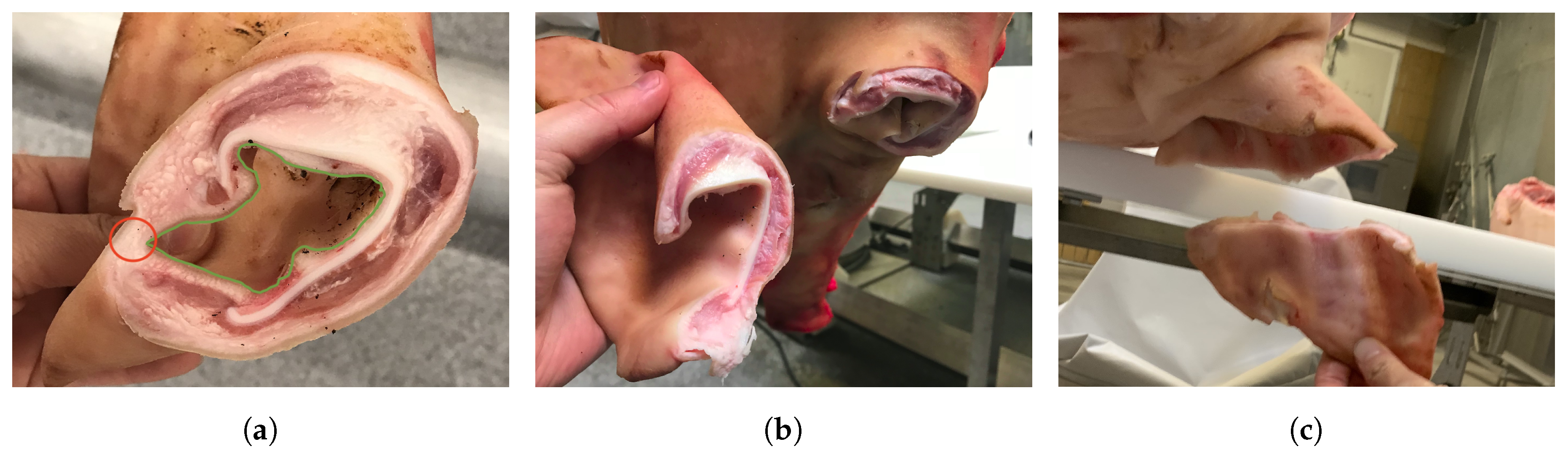
1.1. Case
1.2. Related Work
1.3. Contribution
- A framework for pose prediction from point clouds.
- A novel 5-DoF pose representation for a specific category of tasks.
- Considerations and future work for pose prediction in a challenging setting.
2. Materials and Methods
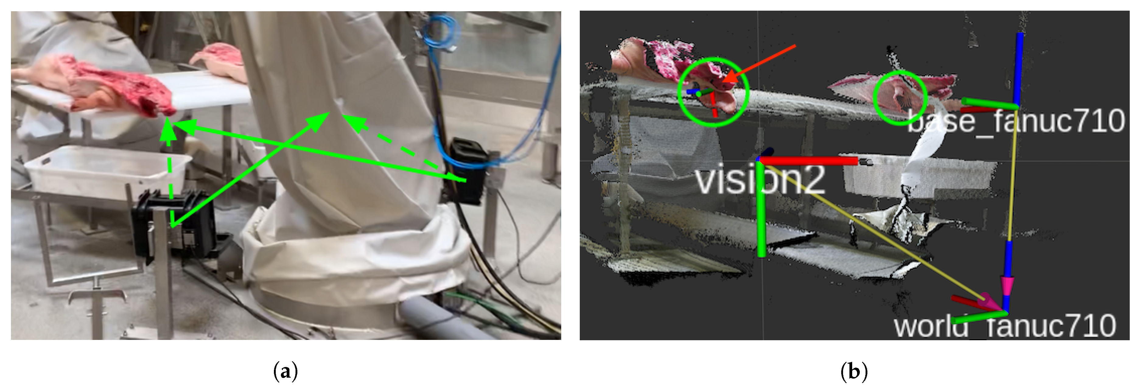
2.1. Sensors
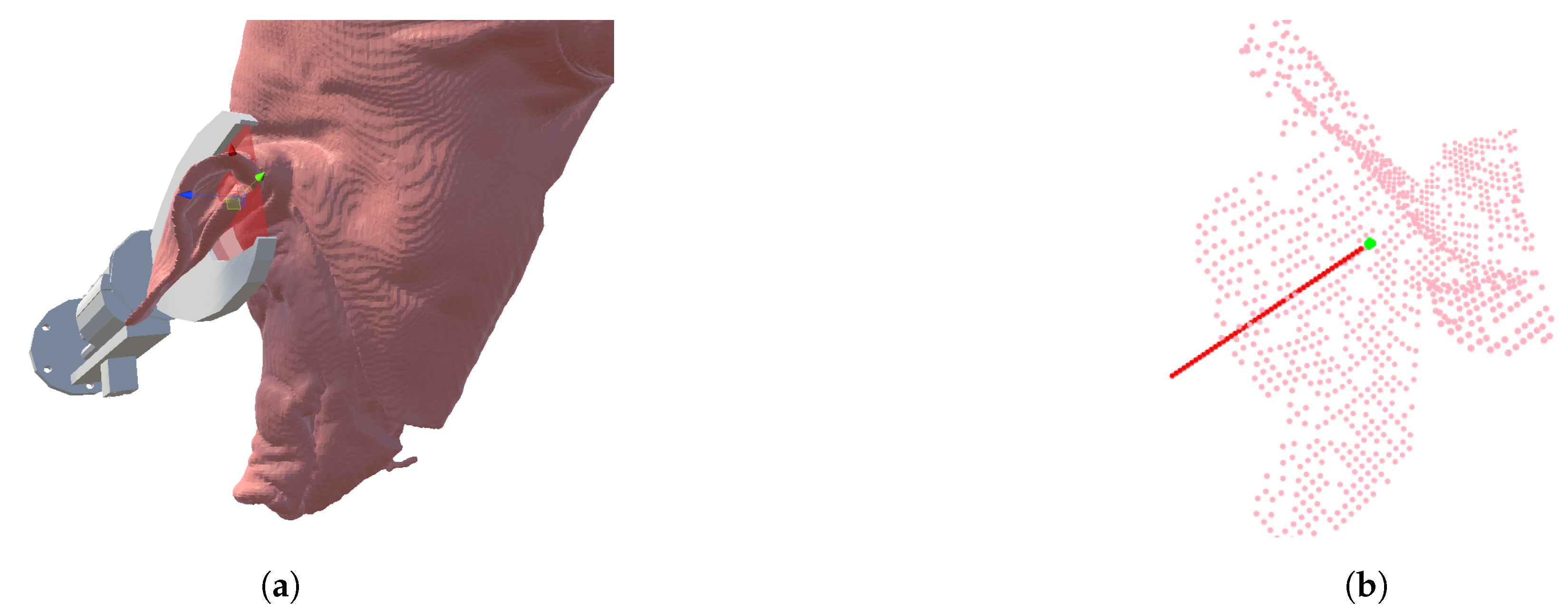
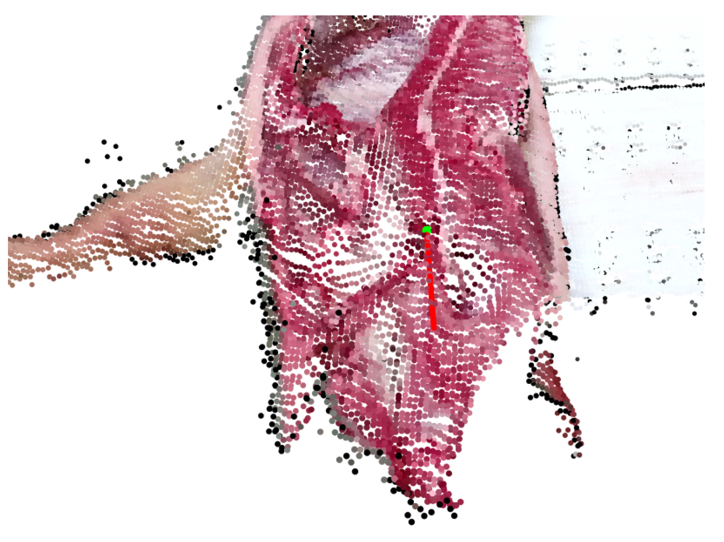
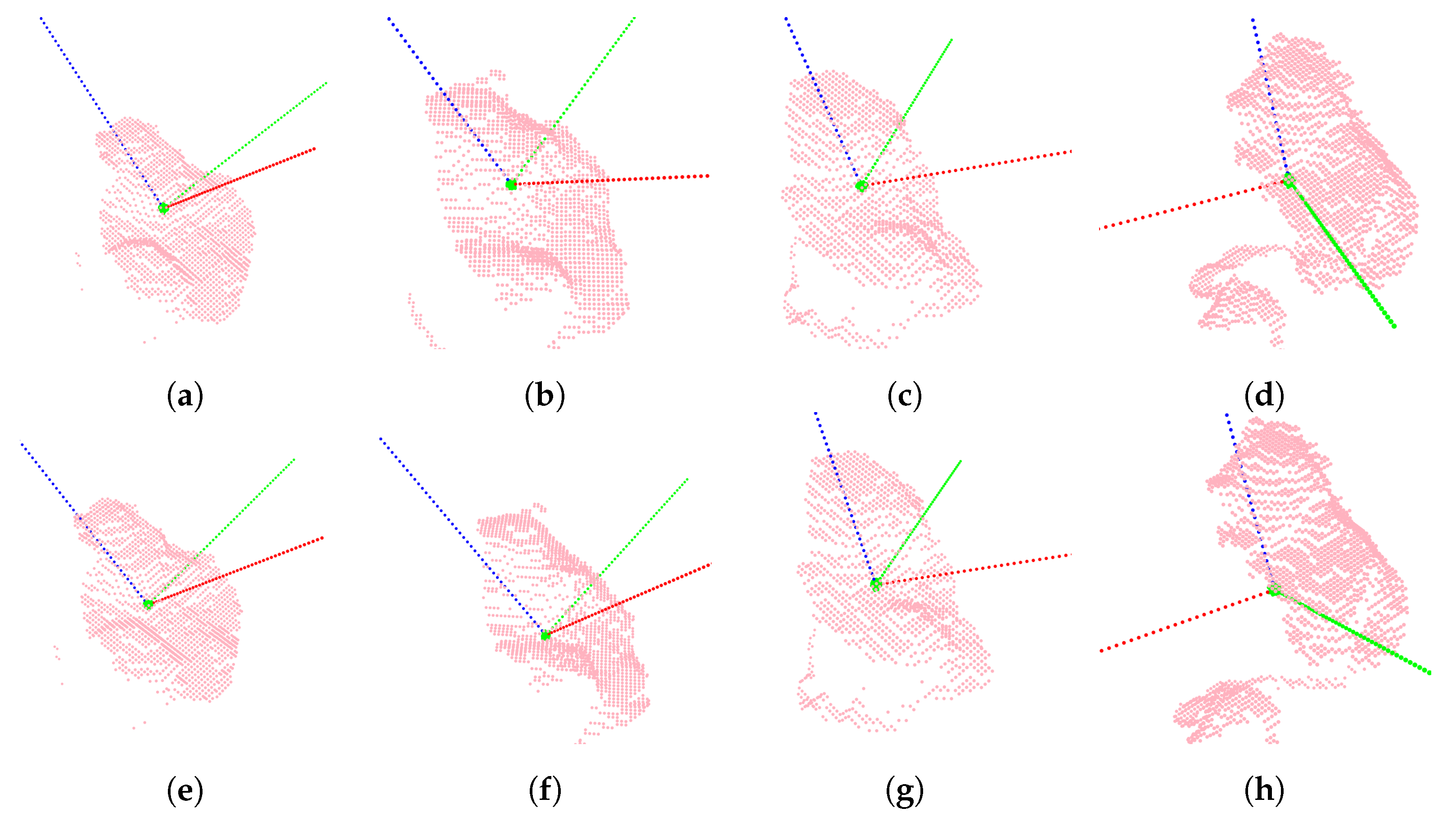
2.2. Tool Pose Representation
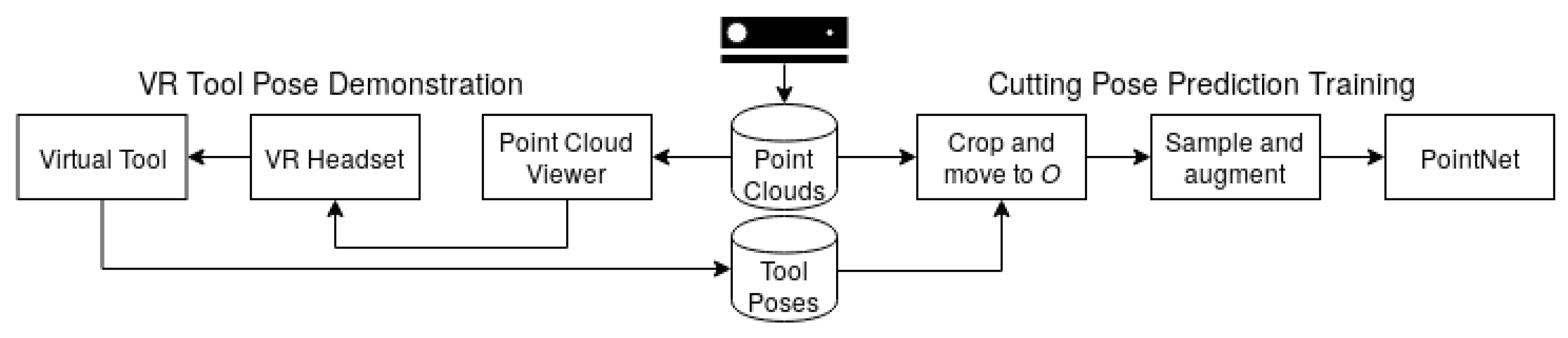
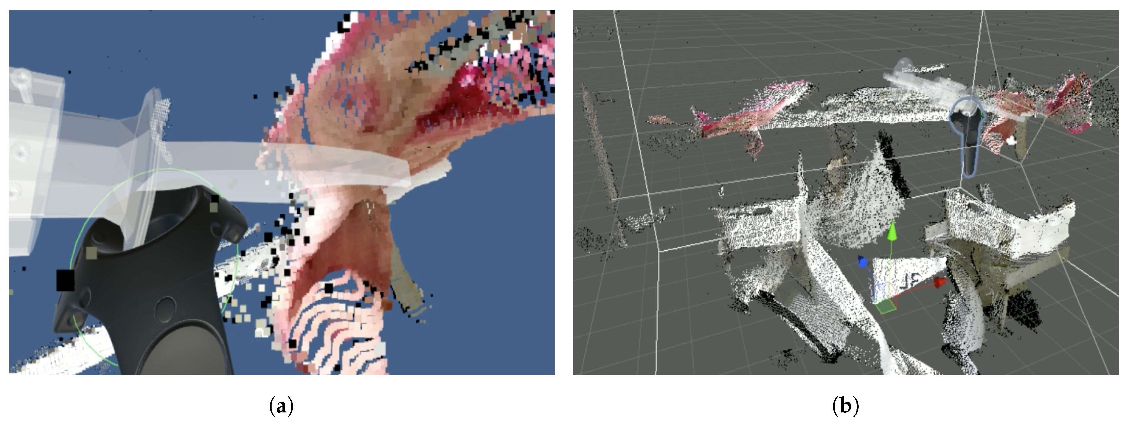
2.3. Demonstration in Virtual Reality
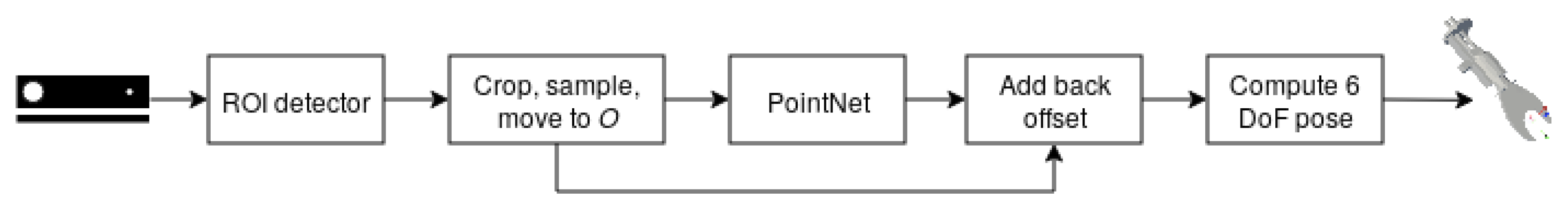
2.4. Region of Interest
2.5. Point Cloud Preprocessing
Cropping
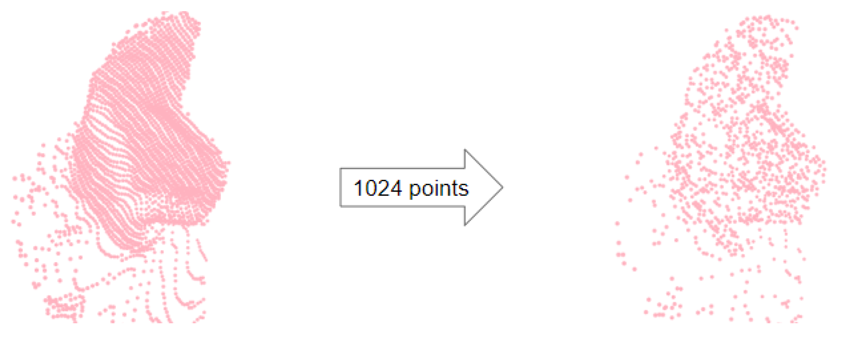
Sampling
Augmentation
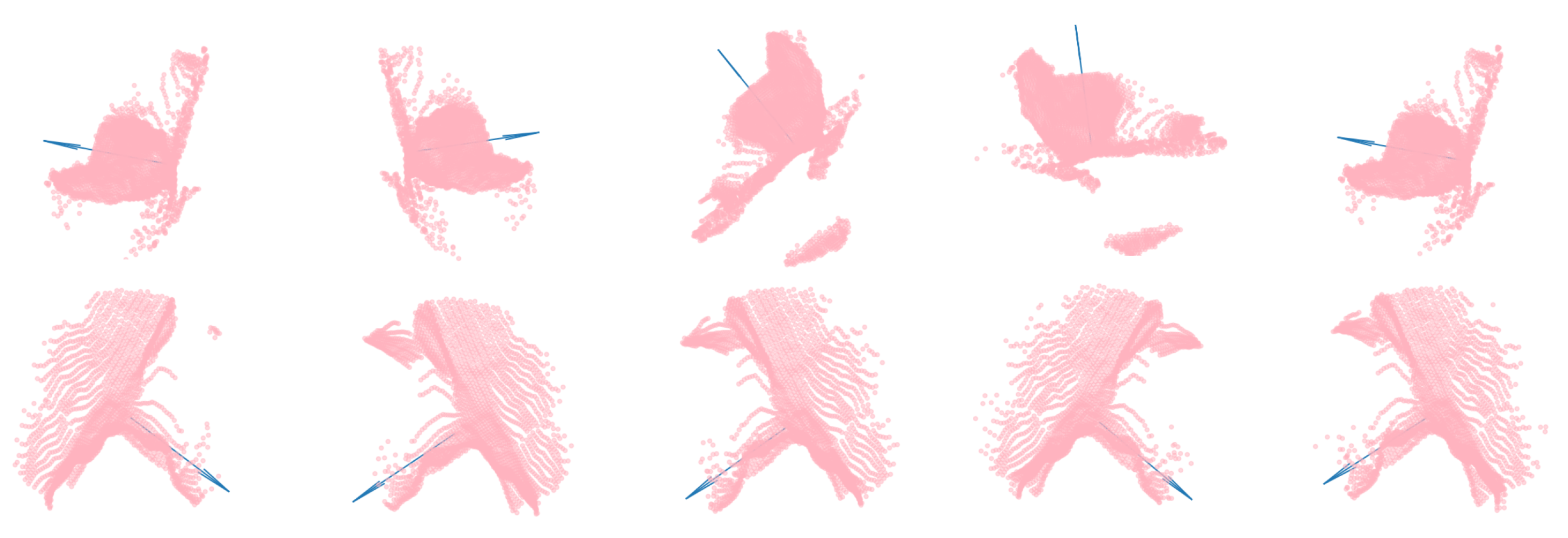
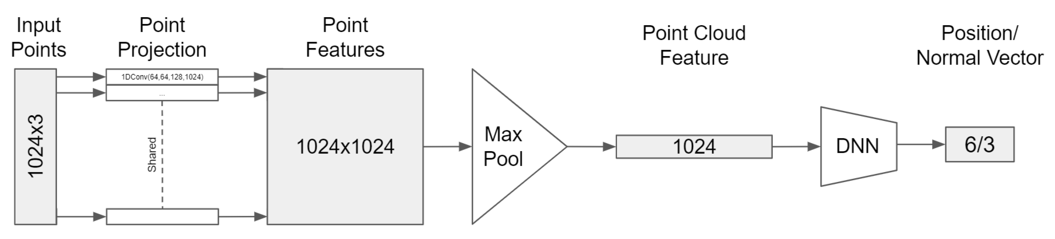
2.6. Cutting Pose Prediction
2.7. Cutting Pose → 6-DoF Tool Pose
3. Results
- Cutting pose prediction performance.
- Network architecture design choices.
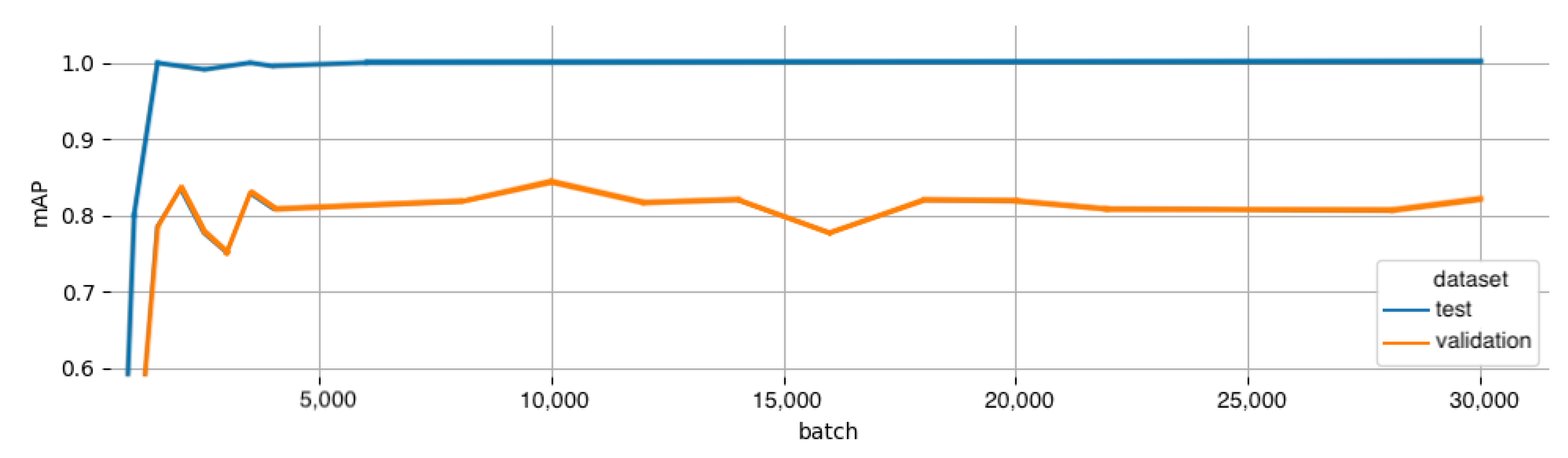
- Impact of training set size.
- Live test in the robot cell.
- Demonstration quality.
- Future applications.
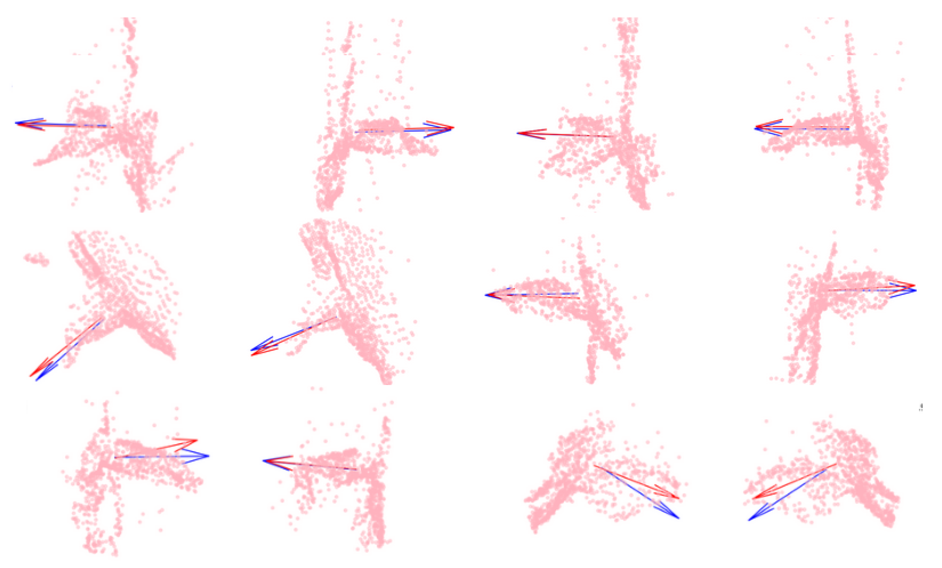
3.1. Cutting Pose Prediction Performance
3.2. Network Architecture Design
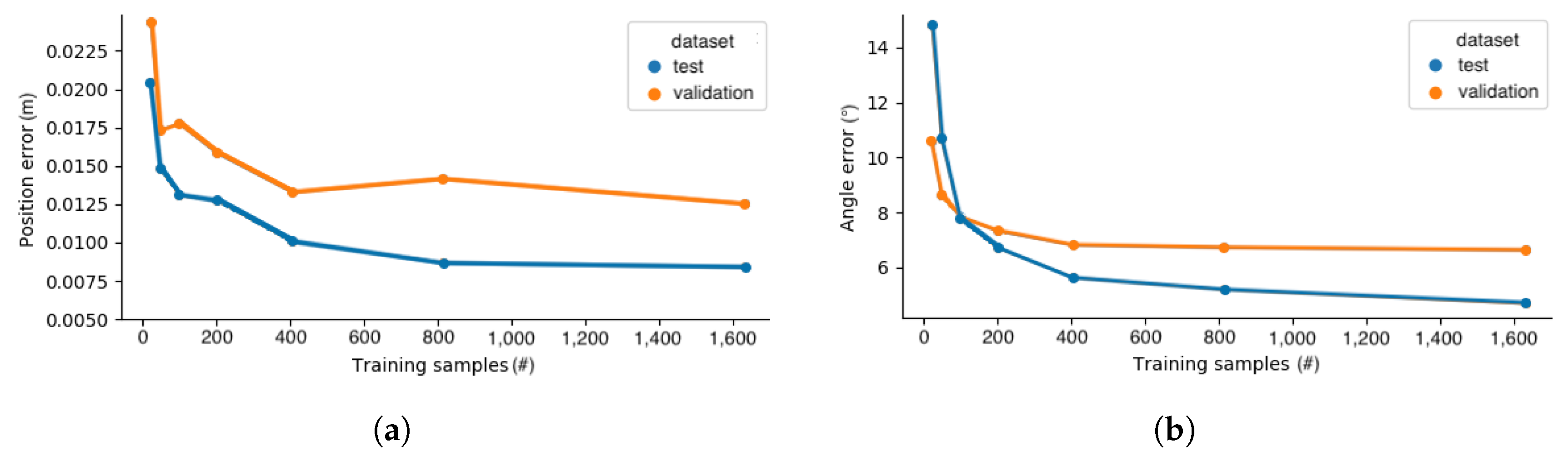
3.3. Training Set Size Impact
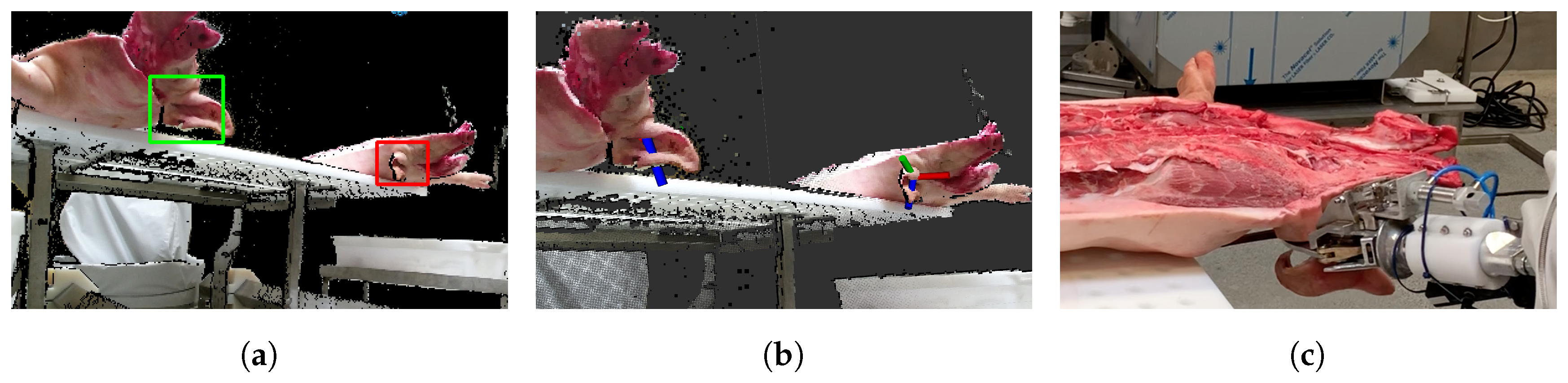
3.4. Live Test
3.5. Quality of Demonstrations
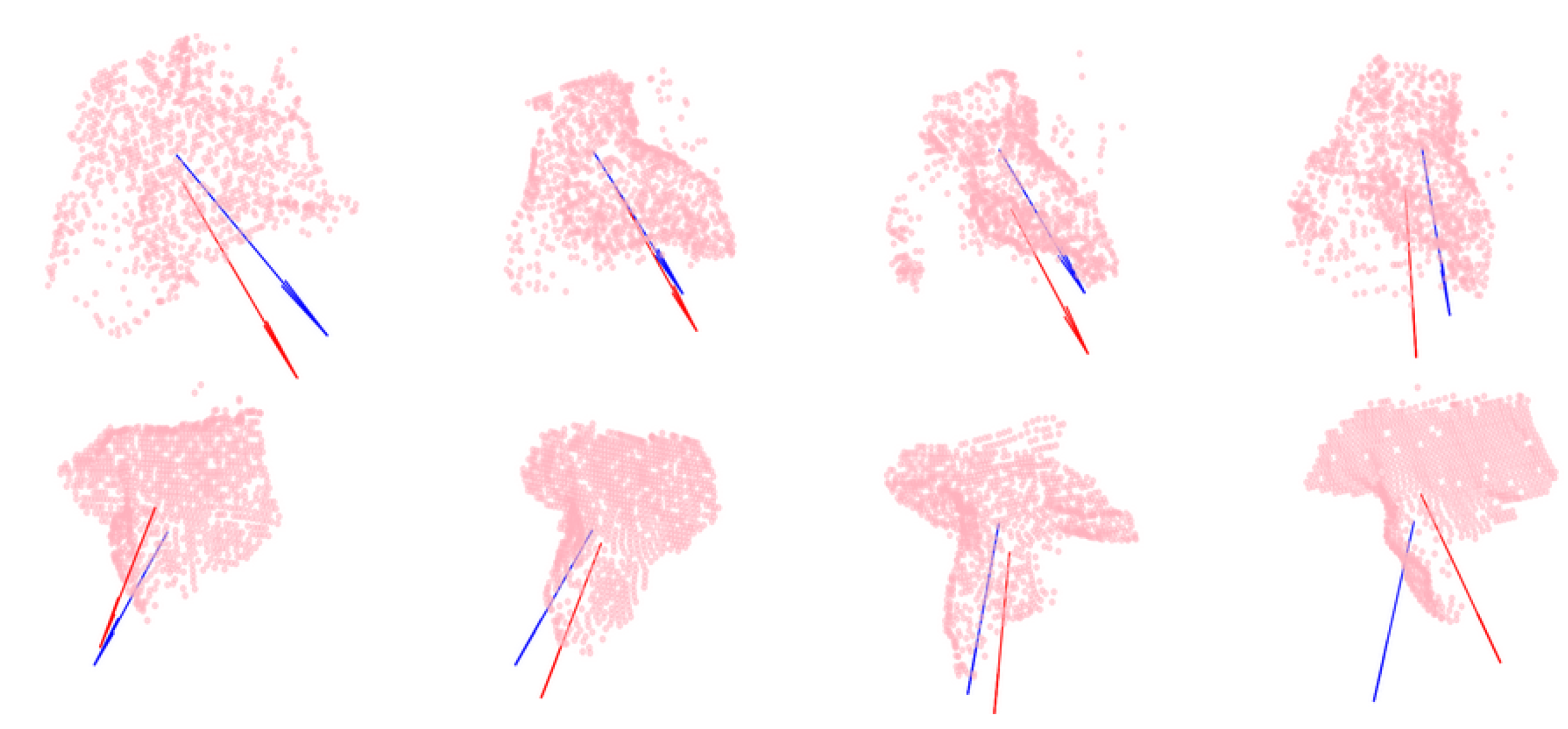
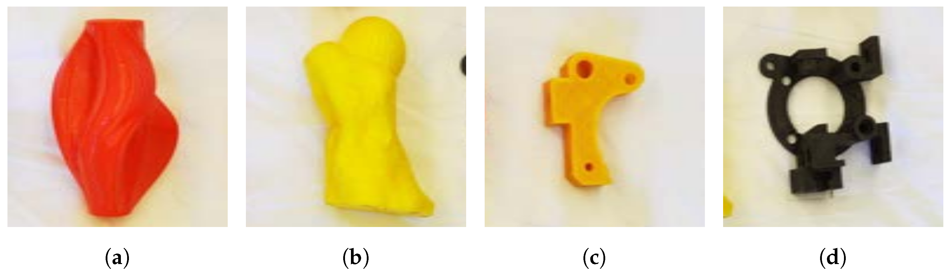
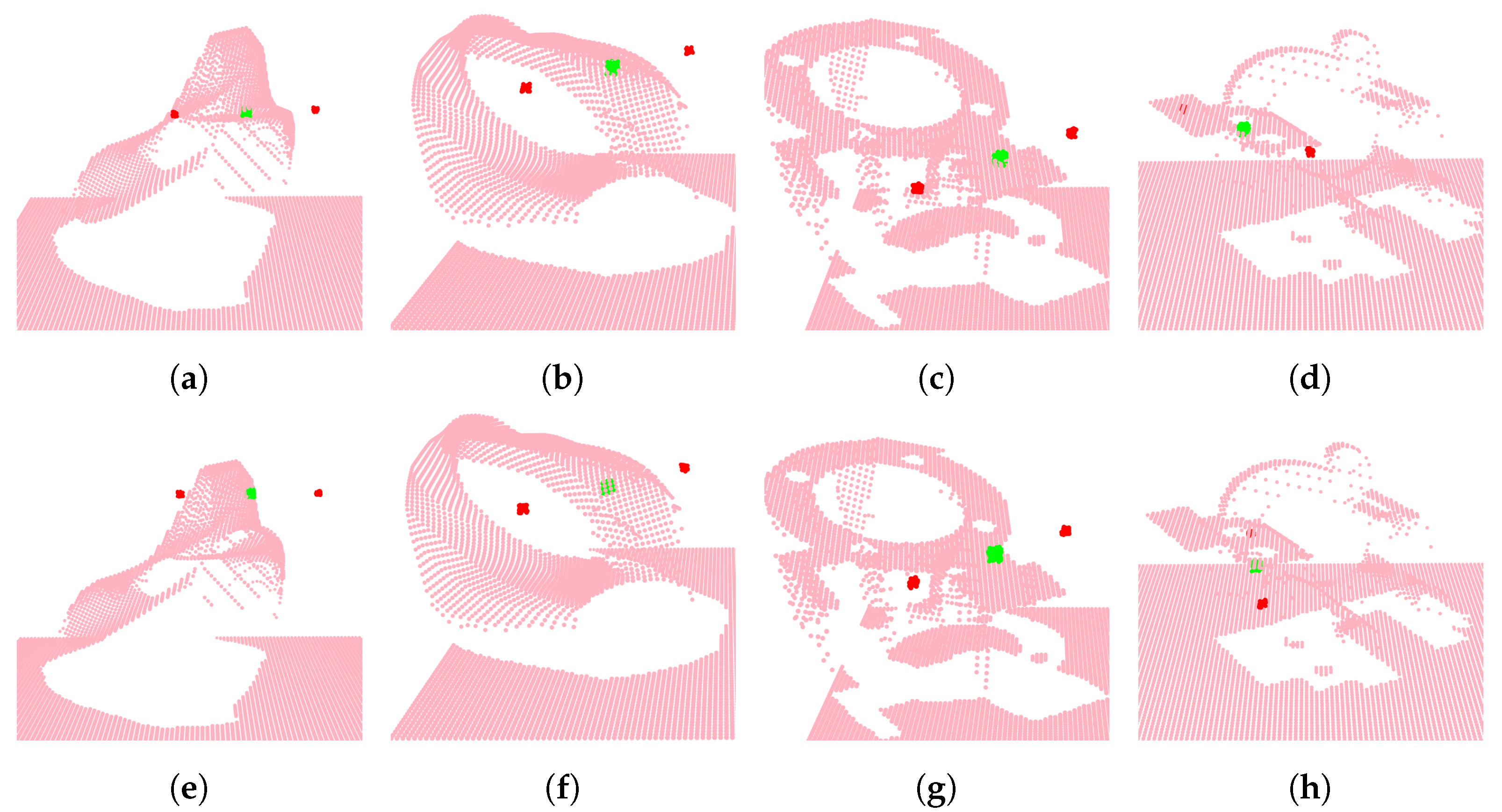
3.6. Generalization of the Method
4. Discussion
Future Work
5. Conclusions
Author Contributions
Funding
Acknowledgments
Conflicts of Interest
Abbreviations
| Convolutional Neural Network | (CNN) |
| Deep Learning | (DL) |
| Deep Neural Networks | (DNN) |
| Degrees of Freedom | (DoF) |
| Fully Convolutional Network | (FCN) |
| Iterative Closest Point | (ICP) |
| Machine Learning | (ML) |
| Mean Average Error | (MAE) |
| Mean Squared Error | (MSE) |
| Perspective-n-Point | (PnP) |
| Region of Interest | (ROI) |
| Virtual Reality | (VR) |
References
- Hassabis, D. Artificial Intelligence: Chess match of the century. Nature 2017, 544, 413. [Google Scholar] [CrossRef]
- Szegedy, C.; Zaremba, W.; Sutskever, I.; Bruna, J.; Erhan, D.; Goodfellow, I.; Fergus, R. Intriguing properties of neural networks. arXiv 2013, arXiv:1312.6199v4. [Google Scholar]
- Alcorn, M.A.; Li, Q.; Gong, Z.; Wang, C.; Mai, L.; Ku, W.; Nguyen, A. Strike (With) a Pose: Neural Networks Are Easily Fooled by Strange Poses of Familiar Objects. In Proceedings of the IEEE Conference on Computer Vision and Pattern Recognition (CVPR), Long Beach, CA, USA, 16–20 June 2019; pp. 4845–4854. [Google Scholar]
- Kohli, M.D.; Summers, R.M.; Geis, J.R. Medical image data and datasets in the era of machine learning—Whitepaper from the 2016 C-MIMI meeting dataset session. J. Digit. Imaging 2017, 30, 392–399. [Google Scholar] [CrossRef] [PubMed]
- Animalia. Meat2.0. 2018. Available online: https://www.animalia.no/no/animalia/om-animalia/arsrapporter-og-strategi/aret-som-gikk–2017/forsker-pa-framtidens-slakterier/ (accessed on 10 March 2020).
- Institute, D.T. Augmented Cellular Meat Production. 2018. Available online: https://www.teknologisk.dk/ydelser/intelligente-robotter-skal-fastholde-koedproduktion-i-danmark/39225 (accessed on 10 March 2020).
- Boylan, W.; Seale, M.; Rahnefeld, G. Ear characteristics and performance in swine. Can. J. Anim. Sci. 1966, 46, 41–46. [Google Scholar] [CrossRef]
- Hinterstoisser, S.; Lepetit, V.; Ilic, S.; Holzer, S.; Bradski, G.; Konolige, K.; Navab, N. Model based training, detection and pose estimation of texture-less 3D objects in heavily cluttered scenes. In Proceedings of the 11th Asian Conference on Computer Vision, Daejeon, Korea, 5–9 November 2012; pp. 548–562. [Google Scholar]
- Hinterstoisser, S.; Holzer, S.; Cagniart, C.; Ilic, S.; Konolige, K.; Navab, N.; Lepetit, V. Multimodal templates for real-time detection of texture-less objects in heavily cluttered scenes. In Proceedings of the 2011 International Conference on Computer Vision, Barcelona, Spain, 6–13 November 2011; pp. 858–865. [Google Scholar]
- Kehl, W.; Manhardt, F.; Tombari, F.; Ilic, S.; Navab, N. SSD-6D: Making RGB-based 3D detection and 6D pose estimation great again. In Proceedings of the IEEE International Conference on Computer Vision (ICCV), Venice, Italy, 22–29 October 2017; pp. 1521–1529. [Google Scholar]
- Xiang, Y.; Schmidt, T.; Narayanan, V.; Fox, D. Posecnn: A convolutional neural network for 6D object pose estimation in cluttered scenes. arXiv 2017, arXiv:1711.00199. [Google Scholar]
- Wong, J.M.; Kee, V.; Le, T.; Wagner, S.; Mariottini, G.L.; Schneider, A.; Hamilton, L.; Chipalkatty, R.; Hebert, M.; Johnson, D.M.S.; et al. SegICP: Integrated Deep Semantic Segmentation and Pose Estimation. In Proceedings of the 2017 IEEE/RSJ International Conference on Intelligent Robots and Systems (IROS), Vancouver, BC, Canada, 24–28 September 2017. [Google Scholar]
- Wang, C.; Xu, D.; Zhu, Y.; Martín, R.; Lu, C.; Fei, L.; Savarese, S. DenseFusion: 6D Object Pose Estimation by Iterative Dense Fusion. In Proceedings of the IEEE Conference on Computer Vision and Pattern Recognition (CVPR), Long Beach, CA, USA, 16–20 June 2019; pp. 3343–3352. [Google Scholar]
- Krull, A.; Brachmann, E.; Michel, F.; Yang, M.; Gumhold, S.; Rother, C. Learning analysis-by-synthesis for 6D pose estimation in RGB-D images. In Proceedings of the IEEE International Conference on Computer Vision (ICCV), Santiago, Chile, 13–16 December 2015; pp. 954–962. [Google Scholar]
- Zeng, A.; Yu, K.T.; Song, S.; Suo, D.; Walker, E., Jr.; Rodriguez, A.; Xiao, J. Multi-view Self-supervised Deep Learning for 6D Pose Estimation in the Amazon Picking Challenge. In Proceedings of the 2017 IEEE International Conference on Robotics and Automation (ICRA), Singapore, 29 May–3 June 2017. [Google Scholar]
- Tekin, B.; Sinha, S.N.; Fua, P. Real-time seamless single shot 6d object pose prediction. In Proceedings of the The IEEE Conference on Computer Vision and Pattern Recognition (CVPR), Salt Lake City, UT, USA, 12–18 June 2018; pp. 292–301. [Google Scholar]
- Hu, Y.; Hugonot, J.; Fua, P.; Salzmann, M. Segmentation-driven 6D object pose estimation. In Proceedings of the IEEE Conference on Computer Vision and Pattern Recognition (CVPR), Long Beach, CA, USA, 16–20 June 2019; pp. 3385–3394. [Google Scholar]
- Saxena, A.; Driemeyer, J.; Ng, A.Y. Robotic grasping of novel objects using vision. Int. J. Rob. Res. 2008, 27, 157–173. [Google Scholar] [CrossRef]
- Fischinger, D.; Vincze, M. Empty the basket-a shape based learning approach for grasping piles of unknown objects. In Proceedings of the 2012 IEEE/RSJ International Conference on Intelligent Robots and Systems, Vilamoura, Portugal, 7–12 October 2012; pp. 2051–2057. [Google Scholar]
- Lenz, I.; Lee, H.; Saxena, A. Deep learning for detecting robotic grasps. Int. J. Rob. Res. 2015, 34, 705–724. [Google Scholar] [CrossRef]
- Pinto, L.; Gupta, A. Supersizing self-supervision: Learning to grasp from 50k tries and 700 robot hours. In Proceedings of the 2016 IEEE international conference on robotics and automation (ICRA), Stockholm, Sweden, 16–21 May 2016; pp. 3406–3413. [Google Scholar]
- Kumra, S.; Kanan, C. Robotic grasp detection using deep convolutional neural networks. In Proceedings of the 2017 IEEE/RSJ International Conference on Intelligent Robots and Systems (IROS), Vancouver, BC, Canada, 24–28 September 2017; pp. 769–776. [Google Scholar]
- Du, G.; Wang, K.; Lian, S. Vision-based Robotic Grasping from Object Localization, Pose Estimation, Grasp Detection to Motion Planning: A Review. arXiv 2019, arXiv:1905.06658. [Google Scholar]
- Sanchez, J.; Corrales, J.A.; Bouzgarrou, B.C.; Mezouar, Y. Robotic manipulation and sensing of deformable objects in domestic and industrial applications: A survey. Int. J. Rob. Res. 2018, 37, 688–716. [Google Scholar] [CrossRef]
- Lin, G.; Tang, Y.; Zou, X.; Xiong, J.; Li, J. Guava detection and pose estimation using a low-cost RGB-D sensor in the field. Sensors 2019, 19, 428. [Google Scholar] [CrossRef]
- ten Pas, A.; Platt, R. Localizing antipodal grasps in point clouds. arXiv 2015, arXiv:1501.03100. [Google Scholar]
- ten Pas, A.; Gualtieri, M.; Saenko, K.; Platt, R. Grasp Pose Detection in Point Clouds. SAGE J. 2017, 13–14, 1455–1473. [Google Scholar] [CrossRef]
- Dyrstad, J.S.; Mathiassen, J.R. Grasping virtual fish: A step towards robotic deep learning from demonstration in virtual reality. In Proceedings of the 2017 IEEE International Conference on Robotics and Biomimetics (ROBIO), Macau, China, 5–8 December 2017; pp. 1181–1187. [Google Scholar]
- Dyrstad, J.S.; Øye, E.R.; Stahl, A.; Mathiassen, J.R. Teaching a Robot to Grasp Real Fish by Imitation Learning from a Human Supervisor in Virtual Reality. In Proceedings of the 2018 IEEE/RSJ International Conference on Intelligent Robots and Systems (IROS), Madrid, Spain, 1–5 October 2018; pp. 7185–7192. [Google Scholar]
- Qi, C.R.; Su, H.; Mo, K.; Guibas, L.J. PointNet: Deep Learning on Point Sets for 3D Classification and Segmentation. In Proceedings of the IEEE Conference on Computer Vision and Pattern Recognition (CVPR), Honolulu, HI, USA, 21–26 July 2017; pp. 652–660. [Google Scholar]
- Liang, H.; Ma, X.; Li, S.; Görner, M.; Tang, S.; Fang, B.; Sun, F.; Zhang, J. PointNetGPD: Detecting Grasp Configurations from Point Sets. In Proceedings of the 2019 International Conference on Robotics and Automation (ICRA), Montreal, QC, Canada, 20–24 May 2019. [Google Scholar]
- Ge, L.; Cai, Y.; Weng, J.; Yuan, J. Hand PointNet: 3D hand pose estimation using point sets. In Proceedings of the IEEE Conference on Computer Vision and Pattern Recognition (CVPR), Salt Lake City, UT, USA, 18–22 June 2018; pp. 8417–8426. [Google Scholar]
- Wiedemeyer, T. IAI Kinect2. 2014–2015. Available online: https://github.com/code-iai/iai_kinect2 (accessed on 10 January 2020).
- Herzog, A.; Pastor, P.; Kalakrishnan, M.; Righetti, L.; Bohg, J.; Asfour, T.; Schaal, S. Learning of grasp selection based on shape-templates. Auton. Robots 2014, 36, 51–65. [Google Scholar] [CrossRef]
- Redmon, J.; Angelova, A. Real-time grasp detection using convolutional neural networks. In Proceedings of the 2015 IEEE International Conference on Robotics and Automation (ICRA), Seattle, WA, USA, 26–30 May 2015; pp. 1316–1322. [Google Scholar]
- Mahler, J.; Liang, J.; Niyaz, S.; Laskey, M.; Doan, R.; Liu, X.; Ojea, J.A.; Goldberg, K. Dex-Net 2.0: Deep Learning to Plan Robust Grasps with Synthetic Point Clouds and Analytic Grasp Metrics. arXiv 2017, arXiv:1703.09312v3. [Google Scholar]
- Mahendran, S.; Ali, H.; Vidal, R. 3D Pose Regression Using Convolutional Neural Networks. In Proceedings of the IEEE International Conference on Computer Vision (ICCV), Venice, Italy, 22–29 October 2017. [Google Scholar]
- Manhardt, F.; Kehl, W.; Navab, N.; Tombari, F. Deep model-based 6d pose refinement in rgb. In Proceedings of the European Conference on Computer Vision (ECCV), Munich, Gemany, 8–14 September 2018; pp. 800–815. [Google Scholar]
- Do, T.; Cai, M.; Pham, T.; Reid, I.D. Deep-6DPose: Recovering 6D Object Pose from a Single RGB Image. arXiv 2018, arXiv:1802.10367v1. [Google Scholar]
- Siemens. ROS#. 2020. Available online: https://github.com/siemens/ros-sharp (accessed on 10 March 2020).
- Technologies, U. Unity. 2020. Available online: https://unity.com (accessed on 10 March 2020).
- Philipsen, M.P.; Wu, H.; Moeslund, T.B. Virtual Reality for Demonstrating Tool Pose. In Proceedings of the 2018 Abstract from Automating Robot Experiments, Madrid, Spain, 5 October 2018. [Google Scholar]
- Redmon, J.; Divvala, S.; Girshick, R.; Farhadi, A. You Only Look Once: Unified, Real-Time Object Detection. In Proceedings of the IEEE Conference on Computer Vision and Pattern Recognition (CVPR), Las Vegas, NV, USA, 26 June–1 July 2016. [Google Scholar]
- Redmon, J.; Farhadi, A. YOLOv3: An Incremental Improvement. arXiv 2018, arXiv:1804.02767v1. [Google Scholar]
- Lin, T.; Maire, M.; Belongie, S.J.; Bourdev, L.D.; Girshick, R.B.; Hays, J.; Perona, P.; Ramanan, D.; Dollár, P.; Zitnick, C.L. Microsoft COCO: Common Objects in Context. In Proceedings of the 13th European Conference, Zurich, Switzerland, 6–12 September 2014. [Google Scholar]
- Atzmon, M.; Maron, H.; Lipman, Y. Point Convolutional Neural Networks by Extension Operators. arXiv 2018, arXiv:1803.10091. [Google Scholar] [CrossRef]
- Sarabandi, S.; Thomas, F. A survey on the computation of quaternions from rotation matrices. J. Mech. Rob. 2019, 11, 021006. [Google Scholar] [CrossRef]
- Sarabandi, S.; Thomas, F. Accurate computation of quaternions from rotation matrices. In Proceedings of the International Symposium on Advances in Robot Kinematics, Bologna, Italy, 1–5 July 2018; pp. 39–46. [Google Scholar]
- Brachmann, E.; Michel, F.; Krull, A.; Yang, M.; Gumhold, S.; Rother, C. Uncertainty-driven 6d pose estimation of objects and scenes from a single rgb image. In Proceedings of the IEEE Conference on Computer Vision and Pattern Recognition (CVPR), Las Vegas, NV, USA, 26 June–1 July 2016; pp. 3364–3372. [Google Scholar]
- Kleppe, A.; Bjørkedal, A.; Larsen, K.; Egeland, O. Automated assembly using 3D and 2D cameras. Robotics 2017, 6, 14. [Google Scholar] [CrossRef]
- Xu, H.; Chen, G.; Wang, Z.; Sun, L.; Su, F. RGB-D-Based Pose Estimation of Workpieces with Semantic Segmentation and Point Cloud Registration. Sensors 2019, 19, 1873. [Google Scholar] [CrossRef]
- Le, T.T.; Lin, C.Y. Bin-Picking for Planar Objects Based on a Deep Learning Network: A Case Study of USB Packs. Sensors 2019, 19, 3602. [Google Scholar] [CrossRef] [PubMed]
- Shotton, J.; Glocker, B.; Zach, C.; Izadi, S.; Criminisi, A.; Fitzgibbon, A. Scene coordinate regression forests for camera relocalization in RGB-D images. In Proceedings of the IEEE Conference on Computer Vision and Pattern Recognition (CVPR), Portland, OR, USA, 25–27 June 2013; pp. 2930–2937. [Google Scholar]
- Hietanen, A.; Latokartano, J.; Foi, A.; Pieters, R.; Kyrki, V.; Lanz, M.; Kämäräinen, J. Benchmarking 6D Object Pose Estimation for Robotics. arXiv 2019, arXiv:1906.02783v2. [Google Scholar]
- Kendall, A.; Grimes, M.; Cipolla, R. Posenet: A convolutional network for real-time 6-dof camera relocalization. In Proceedings of the IEEE international conference on computer vision (ICCV), Santiago, Chile, 13–16 December 2015; pp. 2938–2946. [Google Scholar]
- Rad, M.; Lepetit, V. BB8: A Scalable, Accurate, Robust to Partial Occlusion Method for Predicting the 3D Poses of Challenging Objects without Using Depth. In Proceedings of the IEEE International Conference on Computer Vision (ICCV), Venice, Italy, 22–29 October 2017. [Google Scholar]
- Satish, V.; Mahler, J.; Goldberg, K. On-policy dataset synthesis for learning robot grasping policies using fully convolutional deep networks. IEEE Rob. Autom. Lett. 2019, 4, 1357–1364. [Google Scholar] [CrossRef]
- Ho, J.; Ermon, S. Generative Adversarial Imitation Learning. In Proceedings of the Neural Information Processing Systems 2016, Barcelona, Spain, 5–10 December 2016. [Google Scholar]
- Wu, Z.; Song, S.; Khosla, A.; Yu, F.; Zhang, L.; Tang, X.; Xiao, J. 3d shapenets: A deep representation for volumetric shapes. In Proceedings of the IEEE conference on computer vision and pattern recognition (CVPR), Boston, MA, USA, 8–10 June 2015; pp. 1912–1920. [Google Scholar]
- Chang, A.X.; Funkhouser, T.A.; Guibas, L.J.; Hanrahan, P.; Huang, Q.; Li, Z.; Savarese, S.; Savva, M.; Song, S.; Su, H.; et al. ShapeNet: An Information-Rich 3D Model Repository. arXiv 2015, arXiv:1512.03012v1. [Google Scholar]


| Name | Frames | Unique Instances | From Unique Viewpoint | Samples |
|---|---|---|---|---|
| Train set | 545 | 355 | 724 | 1632 |
| Validation set | 372 | 116 | 158 | 393 |
| Test set | 112 | 75 | 148 | 220 |
| Data Sets | Position Error (std) (m) | Angle Error (std) (°) |
|---|---|---|
| Training | 0.007 (0.003) | 2.025 (1.151) |
| Validation | 0.012 (0.010) | 6.555 (4.942) |
| Test | 0.008 (0.004) | 4.481 (2.692) |
| Position Error (std) (m) | Angle Error (std) (°) | |
|---|---|---|
| Full | 0.014 (0.009) | 6.465 (4.902) |
| Early | 0.020 (0.009) | 6.517 (5.082) |
| Late | 0.029 (0.294) | 6.730 (7.504) |
| Position Error (std) (m) | Angle Error (std) (°) | |
|---|---|---|
| Preliminary | 0.015 (0.008) | 4.592 (2.721) |
| Final | 0.008 (0.004) | 4.481 (2.692) |
| Data Sets | Samples | Position Error (std) (m) | Angle Error (std) (°) |
|---|---|---|---|
| Training | 188 | 0.003 (0.002) | 0.362 (0.229) |
| Validation | 64 | 0.013 (0.007) | 4.566 (2.460) |
| Test | 64 | 0.012 (0.006) | 3.241 (1.775) |
© 2020 by the authors. Licensee MDPI, Basel, Switzerland. This article is an open access article distributed under the terms and conditions of the Creative Commons Attribution (CC BY) license (http://creativecommons.org/licenses/by/4.0/).
Share and Cite
Philipsen, M.P.; Moeslund, T.B. Cutting Pose Prediction from Point Clouds. Sensors 2020, 20, 1563. https://doi.org/10.3390/s20061563
Philipsen MP, Moeslund TB. Cutting Pose Prediction from Point Clouds. Sensors. 2020; 20(6):1563. https://doi.org/10.3390/s20061563
Chicago/Turabian StylePhilipsen, Mark P., and Thomas B. Moeslund. 2020. "Cutting Pose Prediction from Point Clouds" Sensors 20, no. 6: 1563. https://doi.org/10.3390/s20061563
APA StylePhilipsen, M. P., & Moeslund, T. B. (2020). Cutting Pose Prediction from Point Clouds. Sensors, 20(6), 1563. https://doi.org/10.3390/s20061563