Joint Adaptive Sampling Interval and Power Allocation for Maneuvering Target Tracking in a Multiple Opportunistic Array Radar System

Abstract

In this paper, a joint adaptive sampling interval and power allocation (JASIPA) scheme based on chance-constraint programming (CCP) is proposed for maneuvering target tracking (MTT) in a multiple opportunistic array radar (OAR) system. In order to conveniently predict the maneuvering target state of the next sampling instant, the best-fitting Gaussian (BFG) approximation is introduced and used to replace the multimodal prior target probability density function (PDF) at each time step. Since the mean and covariance of the BFG approximation can be computed by a recursive formula, we can utilize an existing Riccati-like recursion to accomplish effective resource allocation. The prior Cramér-Rao lower boundary (prior CRLB-like) is compared with the upper boundary of the desired tracking error range to determine the adaptive sampling interval, and the Bayesian CRLB-like (BCRLB-like) gives a criterion used for measuring power allocation. In addition, considering the randomness of target radar cross section (RCS), we adopt the CCP to package the deterministic resource management model, which minimizes the total transmitted power by effective resource allocation. Lastly, the stochastic simulation is embedded into a genetic algorithm (GA) to produce a hybrid intelligent optimization algorithm (HIOA) to solve the CCP optimization problem. Simulation results show that the global performance of the radar system can be improved effectively by the resource allocation scheme.

1. Introduction

1.1. Background and Motivation

The opportunistic array radar (OAR), proposed by the United States Naval Postgraduate School (NPS), is a new system radar for the next generation naval stealth destroyer DD(X) [1,2,3]. In the OAR system, the stealth of the platform is taken as the core and the digital array is regarded as the base, and then the array elements and the transmit/receive (T/R) modules are placed arbitrarily and aperiodically at available open areas over the entire 3-D space of carrier platforms [4,5]. Due to the unique structure of the antenna array, the resource management of OAR is flexible. On the other hand, the maneuvering target tracking (MTT) plays a vital part for various commercial and military applications and receives plenty of attention [6,7,8,9]. For example, the application areas include battlefield surveillance, air traffic control, air defense, and fire control. Hence, the resource management for MTT in the OAR system is a significant and worthwhile research direction.

So far, many studies has been done to enhance the utilization efficiency of a scarce radar resource in the target tracking process [10,11,12,13,14,15,16]. Reference [10] proposes a sensor selection policy for static target location in distributed multiple-radar architectures. This policy is formulated in a combinatorial optimization framework as a knapsack problem (KP) to obtain a performance level with the lowest cost. Referring to the Bayesian Cramér-Rao lower bound (BCRLB) as a criteria, Reference [11] puts forward a joint power and beams allocation algorithm for multiple target tracking in a co-located multiple input multiple output (MIMO) radar system. Besides, by incorporating an information reduction factor (IRF), the BCRLB is efficiently computed with a measurement origin uncertainty (MOU) and the radar resource is allocated to the targets reasonably in clutter [12]. A joint node selection and power allocation strategy is developed with the objective of tracking multiple targets in Reference [15]. In order to improve the worst-case tracking accuracy with multiple targets, the proposed mechanism implements the optimal resource allocation based on the feedback information in the tracking recursion cycle. In Reference [16], the resource allocation problem concerns the sensor subset, power, and bandwidth. The three-variable optimization problem is simplified by deriving the relationship between the optimal power allocation vector and the bandwidth allocation vector. This algorithm can help achieve better performance within the same resource constraints.

The previously mentioned work provides us with an opportunity, and helps to deal with the resource management problem. However, this work only considers the resource management problems of a uniform moving target [11,12,13,14,15,16]. In the actual battlefield environment, such a favorable circumstance is always an unrealistic assumption. In military applications, the target aircrafts typically fly intelligently in order to achieve their objectives. Even they have electronic equipment that can measure the active sensor’s attempts to track them and may respond accordingly. Therefore, an intelligent resource allocation framework is presented herein for tracking a maneuvering target with Markovian switching dynamics (MSD means that the current target state only depends on the previous target states) in multiple OAR systems. This is a hybrid estimation problem where it is required to estimate sequentially both the continuous-valued target state and the discrete-valued switching model variable. There are several existing error bounds that deal with the hybrid system estimation problem. Examples are Bhattacharyya, Bobrovsky-Zakai, and Weiss-Weinstein lower bounds [17]. However, the derivations of these bounds are extremely complex and their implementation is very involved [18,19]. In addition, the direct application of the BCRLB recursive formula for nonlinear filtering [20] would lead to differentiation of terms involving the discrete-valued model variable. Hence, an approximation to the BCRLB for MSD is considered in this case [21,22,23]. The essence of this technique is to replace the multimodal prior target probability density function (PDF) with a best-fitting Gaussian (BFG) distribution at each time step. The mean and covariance of BFG distribution can be computed through a recursive formula.

In a traditional multiple radar system, prior knowledge is not utilized for a resource allocation scheme. In general, the sampling interval is fixed and the transmitted power of spatially separate radars is equal. Such an operation will definitely result in the inadequate use of the limited time and power resources. In terms of time resource, if the sampling interval is too long, it may lead to a large tracking error, or even lose the target. If the sampling interval is too short, the frequent beam illumination is a waste of the radar resource. Through the BFG approximation, we could determine when to transmit beams to acquire data of the tracked targets. The prior Cramér-Rao lower boundary (prior CRLB-like) can be set as a criterion for an adaptive sampling interval [11]. As a consequence, more tracking tasks can be maintained and more radar resources can be applied to track initiation [24]. Regarding the power resource, based on the prior CRLB-like, the BCRLB-like can be calculated as an error measurement contributing to the intelligent power allocation [20].

Generally speaking, in the traditional work of radar resource management, the radar cross section (RCS) of the illuminated target is considered to be a determined value at each sampling instant [11,12,13,15,16]. Due to the effects of the identity, attitude, position, aspect angle, wave length, and polarization, the RCS of the next sampling instant is uncertainty [25], i.e., the RCS to be estimated obeys a certain distribution. To adequately disclose the uncertainty of RCS, we regard it as a random variable. On account of the randomness of constraint conditions, we introduce chance-constraint programming (CCP) to handle the uncertainty by guaranteeing that the stochastic constraint holds at a specific confidence level [26]. When the confidence level is equal to one, we need to provide a radar resource than in other cases to satisfy the constraints. Yet, it can achieve better tracking performance. However, it is not cost-effective to spend superfluous radar resource on the extremely low probability incident that the RCS takes values at the lower boundary of the distribution range. In addition, to obtain an acceptable tracking error, the confidence level cannot be low either. The confidence level is decided by the environments and desired tracking performance. Therefore, the tracking accuracy could be adjusted flexibly conditioned on different confidence levels. Since we abandon the extreme case that satisfies the constraints conditioned on a very low probability, the resource consumption is reduced strikingly to maintain more tracks.

Through the previously mentioned analysis, we propose a joint adaptive sampling interval and power allocation scheme based on CCP for MTT using BFG in multiple OAR systems. The BFG distribution is presented to replace the multimodal prior target PDF at each time step. In order to realize an adaptive sampling interval, the prior CRLB-like is calculated to decide when to illuminate the target. In conjunction with the data Fisher information matrix (FIM) obtained from distributed radars, the approximation of BCRLB is derived for a maneuvering target with MSD, and it is named BCRLB-like. Conditioned on a specified confidence level, we adopt the CCP to package the deterministic resource management model as the final uncertain model. The whole algorithm can be seen as an intelligent response of a radar system to MTT by perceiving environments. The BCRLB-like is to measure the error for target state estimation, and it provides us a criterion to pre-allocate the radar resource. The optimization problem can be solved by a hybrid intelligent optimization algorithm (HIOA) integrating a stochastic simulation and genetic algorithm (GA).

1.2. Main Contributions and Innovations

The main contributions and innovations of this paper are as follows.

(1)

The BFG approximation is employed so as to allocate the radar resource conveniently. Due to the diversities of motion states of maneuvering targets, it is difficult to predict the target state, and the radar resource allocation has no referenced criterion at the next sampling instant. Guaranteeing that the state vectors have the same mean and covariance under different models, the BFG approximation is introduced to replace the multimodal prior target PDF at each time step. The target state can be predicted easily by a single motion equation, and then accomplish the resource pre-allocation.

(2)

A joint adaptive sampling interval and power allocation scheme is presented. The prior CRLB-like as a measurement criteria is compared with the upper boundary of the given tracking error threshold to determine the next optimal sampling interval. The tracking BCRLB-like is computed for power allocation among the distributed radars. The diagonal elements of BCRLB-like provide a referenced boundary on the variances of the estimation of the target’s hybrid state.

(3)

The CCP is brought in to handle the uncertainty of target information in a resource management model. The target RCS is regarded as a random variable. The CCP balances the radar resource and the tracking performance by adjusting the confidence level. If the target environment is simple or the tracking performance requirement is low, the confidence level could be lowered appropriately to save more resources for other tasks.

The remainder of this paper is structured as follows. In Section 2, we provide the system model for a linear jump Markov system. In Section 3, the CCP model is formulated. By introducing the BFG approximation, the BCRLB-like is derived as the inverse of the Bayesian information matrix (BIM) for MTT. This model integrates the adaptive sampling interval and power allocation in multiple OAR systems. Section 4 proposes the HIOA to solve the model, and two algorithms of target state estimation are given in this section. The simulation results and corresponding analysis are provided in Section 5 to verify the effectiveness of the proposed resource allocation scheme. Lastly, we conclude this paper in Section 6.

2. System Model

Suppose a two-dimensional multiple radar system including M (M ≥ 2) distributed monostatic radars. The qth radar is located at (x_q, y_q) (q = 1, 2, …, M). We assume that: (1) the carrier frequency of each radar is different. (2) There is only a matched filter for the respective transmitted signal. In terms of the two assumptions, each radar receives all the echo signals from the target, but the exclusive matched filter can filter out the echo signals transmitted by the other radars. Hence, each radar operates in a monostatic way. In addition, the centralized tracking is adopted for the above multiple radar systems. All radars generate measurements at each sampling instant and report those measurements to the central fusion center (CFC) [27]. It fuses all the acquired measurements in turn and updates the tracks. The fusion architecture is in Figure 1.

where R_i (i = 1,2,…M) denotes the qth radar.

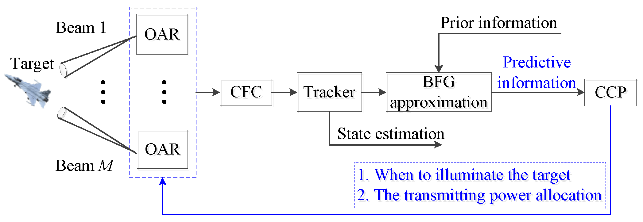
Hence, in accordance with the fusion architecture, the block diagram of a close-loop intelligent tracking system is given in Figure 2.

The tracked target is initially located at (x_T0, y_T0), and the target is located at (x_Tk, y_Tk) at the kth sampling interval. For convenience, the (x_Tk, y_Tk) is denoted as (x_k, y_k).

2.1. Signal Model

It is assumed that the transmitted signal of the qth radar to the target at the kth sample interval is s_q,k(t):

$$s_{q,k}\left(t\right)=\sqrt{P_{q,k}}{S}_{q,k}\left(t\right)\exp \left(-\mathrm{j}2\mathsf{\pi }{f}_q^{\mathrm{c}}t\right)$$

(1)

where P_q,k denotes the transmitted power from the qth radar to the target at the kth sample interval, and $f_q^c$ is the carrier frequency. S_q,k(t) denotes the complex envelope of the transmitted signal.

The baseband representation of the echo signal for the qth radar at the kth sample interval is:

$$r_{q,k}\left(t\right)=h_{q,k}\sqrt{{\alpha }_{q,k}{P}_{q,k}}{S}_{q,k}\left(t-{\tau }_{q,k}\right)\exp \left(-\mathrm{j}2\mathsf{\pi }{f}_{q,k}t\right)+{\varpi }_{q,k}\left(t\right)$$

(2)

where h_q,k denotes the target RCS for the qth radar, and it is a random variable [25]. Furthermore, α_q,k∝1/$R_{q,k}^4$ denotes the variation of the signal strength due to path loss effects along the path of radar q-target-radar q. τ_q,k means time delay and f_q,k is the Doppler frequency. ${\varpi }_{q,k}\left(t\right)$ represents a zero-mean, complex Gaussian white noise with the autocorrelation function ${\sigma }_{\varpi }^2$δ(τ).

2.2. Target Motion Model

As described in previous content, we restrict ourselves to linear jump Markovian systems with an additive Gaussian process noise. Herein, we consider three possible motion models. The three motion models are constant velocity (CV), constant acceleration (CA), and coordinated turn (CT) with a known turn rate, respectively. A larger set of possible motions would be more realistic. Nevertheless, the current set is sufficient to verify the advantage of this algorithm. An overview of other target motion models may be found in References [28,29]. In addition, the dimensionalities of target states for different dynamic models are different, and it may result in a change in the dimensionality of the information matrix, whenever there is a model switch [30]. Hence, to avoid this problem, we set the state vectors with the same dimensionality in different dynamic models. The target state vector consists of the position, velocity, and acceleration in a two-dimensional space. Therefore, the dimensionality of the state vector is six. Details of each motion model used in this paper are given as follows.

2.2.1. Constant Velocity Motion Model

The CV motion model in the xy plane is shown below.

$${\mathsf{\xi }}_k=F_{1,k-1}{\mathsf{\xi }}_{k-1}+w_{1,k-1}$$

(3)

where ${\mathsf{\xi }}_k={\left[x_k {\dot{x}}_k 0 y_k {\dot{y}}_k 0\right]}^{\mathrm{T}}$ denotes the state vector, and its dimension is N_ξ = 6. ${\left[x_k y_k\right]}^{\mathrm{T}}$ and ${\left[{\dot{x}}_{\mathrm{k}} {\dot{y}}_{\mathrm{k}}\right]}^{\mathrm{T}}$ denote the position and velocity of the target, respectively. The acceleration is [0, 0]^T. [•]^T denotes matrix transposition. F_1,k−1 is the 6 × 6 transition matrix.

$$F_{1,k-1}=I_2\otimes \left[\begin{array}{ccc}1& T_k& 0\\ 0& 1& 0\\ 0& 0& 0\end{array}\right]$$

(4)

where $\otimes$ is the Kronecker operator. I₂ denotes an identity matrix of order 2. T_k is the sampling interval (Let k = 0 when the initial time is t = 0, and the first sampling interval T₁ is between k = 0 and k = 1. Thereby, the kth sampling interval between epochs k−1 and k is denoted as T_k in (4). The expression has the same meaning in the remaining paper).

w_1,k−1 represents a zero-mean, complex Gaussian white noise, and its covariance is shown below.

$$Q_{1,k-1}={\sigma }_1•I_2\otimes \left[\begin{array}{ccc}\frac{1}{3}{T}_k^3& \frac{1}{2}{T}_k^2& 0\\ \frac{1}{2}{T}_k^2& T_k& 0\\ 0& 0& 0\end{array}\right]$$

(5)

where σ₁ is the process noise intensity [31].

2.2.2. Constant Acceleration Motion Model

The CA motion model is prescribed as follows.

$${\mathsf{\xi }}_k=F_{2,k-1}{\mathsf{\xi }}_{k-1}+w_{2,k-1}$$

(6)

where ${\mathsf{\xi }}_k={\left[x_k {\dot{x}}_k {\ddot{x}}_k y_k {\dot{y}}_k {\ddot{y}}_k\right]}^{\mathrm{T}}$ denotes the state vector. ${\left[{\ddot{x}}_k {\ddot{y}}_k\right]}^{\mathrm{T}}$ denotes the constant acceleration. F_2,k−1 is the 6 × 6 transition matrix.

$$F_{2,k-1}=I_2\otimes \left[\begin{array}{ccc}1& T_k& \frac{1}{2}{T}_k^2\\ 0& 1& T_k\\ 0& 0& 1\end{array}\right]$$

(7)

w_2,k−1 is a zero-mean, complex Gaussian white noise with the covariance.

$$Q_{2,k-1}={\sigma }_2•I_2\otimes \left[\begin{array}{ccc}\frac{1}{20}{T}_k^5& \frac{1}{8}{T}_k^4& \frac{1}{6}{T}_k^3\\ \frac{1}{8}{T}_k^4& \frac{1}{3}{T}_k^3& \frac{1}{2}{T}_k^2\\ \frac{1}{6}{T}_k^3& \frac{1}{2}{T}_k^2& T_k\end{array}\right]$$

(8)

where σ₂ is the process noise intensity of CA [31].

2.2.3. Coordinated Turn Motion Model

In this scenario, we assume that the angular turn rate Ω is known and constant. Hence, the target motion model of CT remains linear. Then, the CT motion model is expressed as:

$${\mathsf{\xi }}_k=F_{3,k-1}{\mathsf{\xi }}_{k-1}+w_{3,k-1}$$

(9)

where ${\mathsf{\xi }}_k={\left[x_k {\dot{x}}_k 0 y_k {\dot{y}}_k 0\right]}^{\mathrm{T}}$ denotes the state vector. F_3,k−1 is the 6 × 6 transition matrix.

$$F_{3,k-1}=\left[\begin{array}{cccccc}1& \frac{\sin \left(\Omega T_k\right)}{\Omega }& 0& 0& \frac{\cos \left(\Omega T_k\right)-1}{\Omega }& 0\\ 0& \cos \left(\Omega T_k\right)& 0& 0& -\sin \left(\Omega T_k\right)& 0\\ 0& 0& 0& 0& 0& 0\\ 0& \frac{1-\cos \left(\Omega T_k\right)}{\Omega }& 0& 1& \frac{\sin \left(\Omega T_k\right)}{\Omega }& 0\\ 0& \sin \left(\Omega T_k\right)& 0& 0& \cos \left(\Omega T_k\right)& 0\\ 0& 0& 0& 0& 0& 0\end{array}\right]$$

(10)

where Ω is the angular turn rate, and w_3,k−1 is a zero-mean, complex Gaussian white noise with the covariance given by the equation below.

$$Q_{3,k-1}={\sigma }_3•I_2\otimes \left[\begin{array}{ccc}\frac{1}{4}{T}_k^4& \frac{1}{3}{T}_k^3& 0\\ \frac{1}{3}{T}_k^3& \frac{1}{2}{T}_k^2& 0\\ 0& 0& 0\end{array}\right]$$

(11)

where σ₃ is the process noise intensity of CT [31].

2.3. Measurement Model

The measurement equation does not play a role in the BFG approximation. Hence, although the BFG approximation is restricted to linear switching dynamic models, it places no restriction on the measurement equation, which can be nonlinear.

The received signal from the target is an attenuated version of the transmitted signal. The range, azimuth, and Doppler frequency can be extracted from the received signal. The nonlinear measurement equation of the qth radar can be written by the equation below.

$$z_{q,k}=h_{q,k}\left({\mathsf{\xi }}_k\right)+u_{q,k}$$

(12)

where

$$h_{q,k}\left({\mathsf{\xi }}_k\right)={\left(R_{q,k},{\theta }_{q,k},f_{q,k}\right)}^{\mathrm{T}}$$

(13)

with

$$\{\begin{array}{l}{R}_{q.k}=\sqrt{{\left(x_k-x_q\right)}^2+{\left(y_k-y_q\right)}^2}\\ {\theta }_{q,k}=\arctan \left[\left(y_k-y_q\right)/\left(x_k-x_q\right)\right]\\ f_{q,k}=-\frac{2}{{\lambda }_q}\left({\dot{x}}_k,{\dot{y}}_k\right)\cdot {\left(x_k-x_q,y_k-y_q\right)}^{\mathrm{T}}/R_{q.k}\end{array}$$

(14)

corresponding to range, azimuth, and Doppler shift. λ_q is the carrier wavelength of the qth radar. The measurement error u_q,k is a zero-mean Gaussian white noise with the covariance.

$${\mathsf{\Sigma }}_{q,k}=\mathrm{blkdiag}\left({\sigma }_{R_{q,k}}^2 {\sigma }_{{\theta }_{q,k}}^2 {\sigma }_{f_{q,k}}^2\right)$$

(15)

where ${\sigma }_{R_{q,k}}^2$, ${\sigma }_{{\theta }_{q,k}}^2$, and ${\sigma }_{f_{q,k}}^2$ are the BCRLBs of the mean square error (MSE) of the range, azimuth, and Doppler shift at high signal-to-noise ratio (SNR). The BCRLBs for ${\sigma }_{R_{q,k}}^2$ and ${\sigma }_{f_{q,k}}^2$ are given in Chapter 10 of Reference [31], and the BCRLB for ${\sigma }_{{\theta }_{q,k}}^2$ which follows from Reference [32]. The BCRLBs can be described as follows.

$$\{\begin{array}{l}{\sigma }_{R_{q,k}}^2={\mathrm{c}}^2/\left[32{\mathsf{\pi }}^2·SN{R}_{q,k}·{\left(B_{q,k}\right)}^2\right]\\ {\sigma }_{{\theta }_{q,k}}^2=3{\left(B_{\mathrm{NN}}\right)}^2/\left(8{\mathsf{\pi }}^2·SN{R}_{q,k}\right)\\ {\sigma }_{f_{q,k}}^2=3/\left[8{\mathsf{\pi }}^2·SN{R}_{q,k}·{\left(T_{q,k}\right)}^2\right]\end{array}$$

(16)

where B_q,k and T_q,k are the effective bandwidth and effective time duration [31], respectively. B_NN is the null-to-null beam width of the receiver antenna. c is the speed of light. SNR_q,k is the SNR denoted as follows [33].

$$SN{R}_{q,k}=\frac{{\alpha }_{q,k}{\left|h_{q,k}\right|}^2{P}_{q,k}}{{\sigma }_{\varpi }^2}\propto \frac{{\left|h_{q,k}\right|}^2{P}_{q,k}}{{\sigma }_{\varpi }^2{R}_{q,k}^4}$$

(17)

3. Resource Management Model for Maneuvering Target Tracking

${\hat{\mathsf{\xi }}}_k$ is an estimation of the target state ${\mathsf{\xi }}_k$. Hence, ${\hat{\mathsf{\xi }}}_k$ is a function of the measurement value Z_k, which is represented as follows.

$$Z_k={\left\{z_{q,k}\right\}}_{q=1}^M$$

(18)

The performance of any estimator ${\hat{\mathsf{\xi }}}_k$ is measured by the MSE matrix. In the Bayesian estimation, the MSE can be bounded by the BCRLB $C_{\mathrm{BCRLB}}^k$ (defined to be the inverse of BIM J(ξ_k)) in estimating the random vector ${\mathsf{\xi }}_k$, under suitable regularity conditions. For the target with a single motion model, the MSE of any estimator cannot be less than the BCRLB $C_{\mathrm{BCRLB}}^k$ [17].

$${\mathbb{E}}_{{\mathsf{\xi }}_k,{\mathbf{Z}}_k}\left[\right({\hat{\mathsf{\xi }}}_k({\mathbf{Z}}_k)-{\mathsf{\xi }}_k){({\hat{\mathsf{\xi }}}_k(Z_k)-{\mathsf{\xi }}_k)}^{\mathrm{T}}]\ge C_{\mathrm{BCRLB}}^k({\mathsf{\xi }}_k)=J^{-1}({\mathsf{\xi }}_k)$$

(19)

where ${\mathbb{E}}_{{\mathsf{\xi }}_k,Z_k}[·]$ denotes the expectation over ${\mathsf{\xi }}_k$ and Z_k

The BIM $J({\mathsf{\xi }}_k)$ can be described as:

$$J\left({\mathsf{\xi }}_k\right)={\mathbb{E}}_{{\mathsf{\xi }}_k,Z_k}\left[\left(\frac{\partial \ln p\left(Z_k,{\mathsf{\xi }}_k\right)}{\partial {\mathsf{\xi }}_k}\right){\left(\frac{\partial \ln p\left(Z_k,{\mathsf{\xi }}_k\right)}{\partial {\mathsf{\xi }}_k}\right)}^{\mathrm{T}}\right]$$

(20)

The joint PDF p(Z_k,ξ_k) can be factorized as the product of PDF p(ξ_k) and conditional PDF p(Z_k|ξ_k).

$$p\left(Z_k,{\mathsf{\xi }}_k\right)=p\left({\mathsf{\xi }}_k\right)p\left(Z_k|{\mathsf{\xi }}_k\right)$$

(21)

Hence, the BIM J(ξ_k) can be divided into a prior information matrix J_P(ξ_k) and a data information matrix J_D(ξ_k) [17].

$$J\left({\mathsf{\xi }}_k\right)=J_{\mathrm{P}}\left({\mathsf{\xi }}_k\right)+J_{\mathrm{D}}\left({\mathsf{\xi }}_k\right)$$

(22)

The prior information matrix $J_{\mathrm{P}}\left({\mathsf{\xi }}_k\right)$ is determined by the motion equation of targets, and the transmitted power has no impact on it. On the contrary, the data information matrix $J_{\mathrm{D}}\left({\mathsf{\xi }}_k\right)$ is affected by the transmitted power allocated. The larger the transmitted power is, the larger the $J_{\mathrm{D}}\left({\mathsf{\xi }}_k\right)$ is.

3.1. Best-Fitting Gaussian Approximation

To calculate the BIM for linear jump Markovian systems with additive Gaussian process noise through Equation (22), we need to express the dynamics of the system.

$${\mathsf{\xi }}_k=F_{k-1}^{r_k}{\mathsf{\xi }}_{k-1}+w_{k-1}^{r_k},\hspace{1em}{w}_{k-1}^{r_k}~\mathcal{N}\left(0,Q_{\mathrm{p},k-1}^{r_k}\right)$$

(23)

with the BFG approximation:

$${\mathsf{\xi }}_k\approx {\mathsf{\Phi }}_{k-1}{\mathsf{\xi }}_{k-1}+W_{k-1},\hspace{1em}{W}_{k-1}~\mathcal{N}(0,Q_{\mathrm{p},k-1})$$

(24)

where r_k (r_k = 1, 2, …, N_m and N_m is the number of the target motion models) specifies the target motion model in effect during the time interval between sampling time indexes k−1 and k. Φ_k−1, W_k−1, and Q_p,k−1 are the transition matrix, process noise vector, and covariance matrix of the BFG approximation equation, respectively. For convenient representation in the following process of derivation, the notation F_i,k and Q_i,k in Section 2.2 (i = 1, 2, …, N_m) are changed to $F_{k-1}^{r_k}$ and $Q_{\mathrm{p},k-1}^{r_k}$. is an additive Gaussian process noise with ${\mathbf{W}}_{k-1}^{r_k}~\mathcal{N}\left(0,{\mathbf{Q}}_{\mathrm{p},k-1}^{r_k}\right)$.

At each sampling interval, the regime-dependent motion model (given by Equation (23) and known as “model 1”) is replaced with a single BFG distribution (denoted by Equation (24) and referred to as “model 2”). Φ_k−1 and Q_p,k−1 (Q_p,k−1 ≥ 0) are calculated to satisfy the requirements that the distribution of ${\mathsf{\xi }}_k$ has the same mean and covariance under different models at each stage.

$$\mathbb{E}\left[{\mathsf{\xi }}_k|\mathrm{model} 1\right]=\mathbb{E}\left[{\mathsf{\xi }}_k|\mathrm{model} 2\right]$$

(25)

$$\mathrm{Cov}\left[{\mathsf{\xi }}_k|\mathrm{model} 1\right]=\mathrm{Cov}\left[{\mathsf{\xi }}_k|\mathrm{model} 2\right]$$

(26)

where $\mathbb{E}$[•] and Cov[•] denote the expectation operator and covariance operator, respectively.

The computation procurement of Φ_k−1 is given in Appendix A. Then, with the aid of Φ_k−1, we obtain Q_p,k−1 by the detailed derivation in Appendix B.

$${\mathsf{\epsilon }}_k\triangleq \mathbb{E}\left[{\mathsf{\xi }}_k|\mathrm{model} 1\right]=\mathbb{E}\left[{\mathsf{\xi }}_k|\mathrm{model} 2\right]$$

(27)

$${𝓒}_k\triangleq \mathrm{Cov}\left[{\mathsf{\xi }}_k|\mathrm{model} 1\right]=\mathrm{Cov}\left[{\mathsf{\xi }}_k|\mathrm{model} 2\right]$$

(28)

It is assumed that the initial distribution of state vector ξ is Gaussian with mean ${\overline{\mathsf{\xi }}}_0$ and covariance $J_{\mathrm{P}}^{-1}\left({\mathsf{\xi }}_0\right)$. Generally speaking, initially, the target is in a CV motion. Hence, the ε₁ and 𝓒₁ can be calculated easily. The transition probability is p_ij $\triangleq$ Pr(r_k = j|r_k−1 = i) (i, j = 1, 2, …, N_m). To proceed, the recursive computation procedure for Φ_k−1 and Q_p,k−1 is given as follow:

Step 1. Let k = 1, and initialize ε_k−1, 𝓒_k−1, and the mode probabilities p_k−1(r), r = 1, 2, …, N_m

Step 2. Calculate the mode probabilities.

$$p_k(r)={\displaystyle \sum _{j=1}^{N_m}{p}_{jr}{p}_{k-1}(j)}$$

(29)

Step 3. By derivation, obtain Φ_k−1 of BFG distribution as (see Appendix A):

$${\mathsf{\Phi }}_{k-1}=\left[{\displaystyle \sum _{r=1}^{N_m}{F}_{k-1}^r{p}_k\left(r\right)}\right]$$

(30)

Step 4. With the aid of Φ_k−1, derive the covariance matrix 𝓒_k.

$${𝓒}_k={\displaystyle \sum _{r=1}^{N_{\mathrm{m}}}{p}_k\left(r\right)\left[F_{k-1}^r\left({𝓒}_{k-1}+{\mathsf{\epsilon }}_{k-1}{\mathsf{\epsilon }}_{k-1}^{\mathrm{T}}\right){\left(F_{k-1}^r\right)}^{\mathrm{T}}+Q_{k-1}^r\right]}-{\mathsf{\Phi }}_{k-1}{\mathsf{\epsilon }}_{k-1}{\mathsf{\epsilon }}_{k-1}^{\mathrm{T}}{\mathsf{\Phi }}_{k-1}^{\mathrm{T}}$$

(31)

Step 5. Calculate Q_p,k−1 as follows:

$$Q_{\mathrm{p},k-1}={𝓒}_k-{\mathsf{\Phi }}_{k-1}{𝓒}_{k-1}{\mathsf{\Phi }}_{k-1}^{\mathrm{T}}$$

(32)

Step 6. Update the mean of the state vector.

$${\mathsf{\epsilon }}_k={\mathsf{\Phi }}_{k-1}{\mathsf{\epsilon }}_{k-1}$$

(33)

Step 7. Let k = k + 1, and go to Step 2.

3.2. Prior Information J_P(ξ_k)

The prior information matrix J_P(ξ_k) can be formulated by the equation below [20].

$$J_{\mathrm{P}}\left({\mathsf{\xi }}_k\right)={\mathbb{E}}_{{\mathsf{\xi }}_k}\left[\left(\frac{\partial \ln p\left({\mathsf{\xi }}_k\right)}{\partial {\mathsf{\xi }}_k}\right){\left(\frac{\partial \ln p\left({\mathsf{\xi }}_k\right)}{\partial {\mathsf{\xi }}_k}\right)}^{\mathrm{T}}\right]=D_{k-1}^{22}-D_{k-1}^{21}{\left[J\left({\mathsf{\xi }}_{k-1}\right)+D_{k-1}^{11}\right]}^{-1}{D}_{k-1}^{12}$$

(34)

According the calculated Φ_k−1 and Q_p,k−1 by the linear BFG approximation, the $D_{k-1}^{11}$, $D_{k-1}^{12}$, and $D_{k-1}^{22}$ are deterministic and the expectation operator can be dropped out.

$$\{\begin{array}{l}{D}_{k-1}^{11}={\mathsf{\Phi }}_{k-1}^{\mathrm{T}}{Q}_{\mathrm{p},k-1}{\mathsf{\Phi }}_{k-1}\\ D_{k-1}^{12}=-{\mathsf{\Phi }}_{k-1}^{\mathrm{T}}{\left[Q_{\mathrm{p},k-1}\right]}^{-1}\\ D_{k-1}^{22}={\left[Q_{\mathrm{p},k-1}\right]}^{-1}\end{array}$$

(35)

Substituting (35) into (34), we can derive the prior information matrix.

$$J_{\mathrm{P}}\left({\mathsf{\xi }}_k\right)={\left[Q_{\mathrm{p},k-1}+{\mathsf{\Phi }}_{k-1}{J}^{-1}\left({\mathsf{\xi }}_{k-1}\right){\mathsf{\Phi }}_{k-1}^{\mathrm{T}}\right]}^{-1}$$

(36)

3.3. Data Information J_D(ξ_k)

On the other hand, the data information matrix J_D(ξ_k) can be expressed by the equation below [20].

$$J_{\mathrm{D}}\left({\mathsf{\xi }}_k\right)={\mathbb{E}}_{{\mathsf{\xi }}_k,Z_k}\left[\left(\frac{\partial \ln p\left(Z_k|{\mathsf{\xi }}_k\right)}{\partial {\mathsf{\xi }}_k}\right){\left(\frac{\partial \ln p\left(Z_k|{\mathsf{\xi }}_k\right)}{\partial {\mathsf{\xi }}_k}\right)}^{\mathrm{T}}\right]$$

(37)

Since the measurements from different radars are independent from each other, J_D(ξ_k) can be written as follows.

$$\begin{array}{l}{J}_{\mathrm{D}}\left({\mathsf{\xi }}_k\right)={\displaystyle \sum _{q=1}^M{J}_{\mathrm{D}}^q\left({\mathsf{\xi }}_k\right)}\\ ={\displaystyle \sum _{q=1}^M{\mathbb{E}}_{{\mathsf{\xi }}_k,z_{q,k}}\left[\left(\frac{\partial \ln p\left(z_{q,k}|{\mathsf{\xi }}_k\right)}{\partial {\mathsf{\xi }}_k}\right){\left(\frac{\partial \ln p\left(z_{q,k}|{\mathsf{\xi }}_k\right)}{\partial {\mathsf{\xi }}_k}\right)}^{\mathrm{T}}\right]}\\ ={\displaystyle \sum _{q=1}^M{\mathbb{E}}_{{\mathsf{\xi }}_k}\left[H_{q,k}^{\mathrm{T}}{\Sigma }_{q,k}^{-1}{H}_{q,k}\right]}\end{array}$$

(38)

where $H_{q,k}={\left[\partial h_q^{\mathrm{T}}\left({\mathsf{\xi }}_k\right)/\partial {\mathsf{\xi }}_k\right]}^{\mathrm{T}}$.

Substituting Equations (36) and (38) into Equation (22), we can now calculate the BIM J(ξ_k) by using the Riccati-like recursion [20].

$$J\left({\mathsf{\xi }}_k\right)={\left[Q_{\mathrm{p},k-1}+{\mathsf{\Phi }}_{k-1}{J}^{-1}\left({\mathsf{\xi }}_{k-1}\right){\mathsf{\Phi }}_{k-1}^{\mathrm{T}}\right]}^{-1}+{\displaystyle \sum _{q=1}^M{\mathbb{E}}_{{\mathsf{\xi }}_k}\left[H_{q,k}^{\mathrm{T}}{\Sigma }_{q,k}^{-1}{H}_{q,k}\right]}$$

(39)

In practice, the expected value in Equation (39) may be evaluated using Monte Carlo techniques. To shorten the computation time, the predictive BIM is approximated as follows [34].

$$J\left({\mathsf{\xi }}_k\right)={\left[Q_{\mathrm{p},k-1}+{\mathsf{\Phi }}_{k-1}{J}^{-1}\left({\mathsf{\xi }}_{k-1}\right){\mathsf{\Phi }}_{k-1}^{\mathrm{T}}\right]}^{-1}+{\left({\displaystyle \sum _{q=1}^M{H}_{q,k}^{\mathrm{T}}{\Sigma }_{q,k}^{-1}{H}_{q,k}}\right)|}_{{\mathsf{\xi }}_{k|k-1}}$$

(40)

where ξ_k|k−1 denotes the predicted target state for the case of zero process noise.

3.4. Predictive Bayesian Cramér-Rao lower bound (BCRLB-like)

The key feature of the resource allocation algorithm is the predictability. The predictive target tracking performance gives us the ability to make decisions in advance based on current knowledge. In the maneuvering target tracking, Φ_k−1 and Q_p,k−1 are updated through Equations (30) and (32) before each revisit time. They are both functions of the sampling interval T_k. Hence, the mathematical symbol of the prior information matrix can be modified from J_P(ξ_k) to J_P(T_k)|_ξk (J_P(T_k) has nothing to do with ξ_k. Nevertheless, to keep the consistency of the format, it is denoted as $J_P\left(T_k\right)|{ }_{{\mathsf{\xi }}_k}$ here). The data information matrix is affected by the transmitted power of the radars and the target RCS. The larger the transmitted power P_k and the RCS h_k are, the larger the data information matrix is. Consequently, the data information matrix can be rewritten as J_D(P_k,h_k)|_ξk. Considering the updated BIM J(ξ_k−1), sampling interval T_k, transmitted power P_k and RCS h_k, we can calculate the predictive BIM.

$$\begin{array}{cc}\hfill {J\left(T_k,P_k,h_k\right)|}_{{\mathsf{\xi }}_k}& ={J_{\mathrm{P}}\left(T_k\right)|}_{{\mathsf{\xi }}_k}+{J_{\mathrm{D}}\left(P_k,h_k\right)|}_{{\mathsf{\xi }}_k}\hfill \\ \hfill & ={\left[Q_{\mathrm{p},k-1}\left(T_k\right)+{\mathsf{\Phi }}_{k-1}\left(T_k\right)J^{-1}\left({\mathsf{\xi }}_{k-1}\right){\mathsf{\Phi }}_{k-1}^{\mathrm{T}}\left(T_k\right)\right]}^{-1}+{\left[{\displaystyle \sum _{q=1}^M{H}_{q,k}^{\mathrm{T}}{\Sigma }_{q,k}^{-1}\left(P_{q,k},h_k^q\right)H_{q,k}}\right]|}_{{\mathsf{\xi }}_{k|k-1}}\hfill \end{array}$$

(41)

where the meaning of ξ_k|k−1 refers to Equation (40).

The predictive target tracking performance can be calculated as the inverse of BIM. However, because of the BFG approximation technique involved, the predictive target tracking performance no longer provides a lower boundary on error performance. Hence, the predictive target tracking performance in this paper is named BCRLB-like instead of BCRLB.

$${{\mathbf{C}}_{\mathrm{BCRLB}-\mathrm{like}}\left(T_k,P_k,h_k\right)|}_{{\mathsf{\xi }}_k}={\left[{J\left(T_k,P_k,h_k\right)|}_{{\mathsf{\xi }}_k}\right]}^{-1}$$

(42)

The diagonal elements of BCRLB-like provide a referenced boundary on the variances of the estimation of the target’s hybrid state. It is sufficient for us to utilize the tracking BCRLB-like factor of the illuminated target as a criterion for power allocation.

$$F\left(T_k,P_k,h_k\right)=\sqrt{\mathrm{trace}\left[{C_{\mathrm{BCRLB}-\mathrm{like}}\left(T_k,P_k,h_k\right)|}_{{\mathsf{\xi }}_k}\right]}$$

(43)

where Equation (43) denotes the integrated tracking performance of multiple radars at the kth sampling instant.

Having the tracking BCRLB-like F(T_k,P_k,h_k), we can allocate the power resource reasonably while the beams illuminate the target. However, due to the scarce radar resource, the radars do not have to illuminate the target continually. The beams only need to be transmitted when the tracking error is larger than a given tracking error threshold. As shown in Equations (22) and (36), the prior information matrix $J_{\mathrm{P}}\left(T_k\right)$ is only related to a target motion equation. Therefore, the inverse of $J_{\mathrm{P}}\left(T_k\right)$ is utilized to determine when to transmit the beams.

$$C_{\mathrm{CRLB}-\mathrm{like}}^{\mathrm{P}}\left(T_k\right)={\left[{J_{\mathrm{P}}\left(T_k\right)|}_{{\mathsf{\xi }}_k}\right]}^{-1}$$

(44)

To accomplish an adaptive sampling interval, the prior CRLB-like is compared with the upper boundary of the given tracking error threshold. It can be used as a criterion to determine the optimal sampling period. The representation of the prior CRLB-like factor is given as follows.

$$F_{\mathrm{P}}\left(T_k\right)=\sqrt{\mathrm{trace}\left[C_{\mathrm{CRLB}-\mathrm{like}}^{\mathrm{P}}\left(T_k\right)\right]}$$

(45)

3.5. Modeling of Chance-Constraint Programming (CCP)

In accordance with Equation (16), it can be seen that the target tracking accuracy is impacted by several parameters. The decision variables involved in this paper are the sampling interval T_k and the transmit power P_k. The random vector is the RCS h_k. For the predetermined tracking error range at each sampling instant, the aim of our work is to minimize the transmitted power by optimally allocating the limited time and power resources.

$$\begin{array}{cc}\hfill \min & {\mathbf{1}}_M^{\mathrm{T}}{P}_k\hfill \\ \hfill s.t.& \hfill \\ \hfill & P_{q,k}\ge P_{\min }\hspace{1em}q=1,2,\cdots ,M\hfill \\ \hfill & {\mathbf{1}}_M^{\mathrm{T}}{P}_k\le P_{\mathrm{total}}\hfill \\ \hfill & F\left(T_k,P_k,h_k\right)\le {\eta }_{1,k}\hspace{1em}\mathrm{if} F_{\mathrm{P}}\left(T_k\right)\ge {\eta }_{2,k}\hfill \end{array}$$

(46)

where $1_M^T$ = [1,1,…,1]_1×M. P_min is the lower boundary of the transmitted power of each beam. P_total is the available total power. η_1,k and η_2,k are the lower boundary and upper boundary of the tracking error range, respectively. The adaptive sampling interval is included in the resource management model. If the prior CRLB-like F_P(T_k) of the next sampling instant is greater than the given tracking error threshold η_2,k, T_k is set as the sampling interval and the beams are transmitted to track the target.

In Equation (46), the model can make sure that the tasks can be accomplished by as many as possible conditions on the given tracking error threshold.

In practice, the target RCS is related to the identification, attitude, and position of the target, and it is affected by an aspect angle, wavelength, and polarization, etc. [25], i.e., the target RCS is unknown and uncertain. Consequently, the target RCS is considered as a random variable in this paper. Then the deterministic resource allocation model cannot show the characteristic of the target well. In view of the above situation, the stochastic CCP of the resource management is introduced [26]. According to Equation (46), the resource management model can be reformulated as:

$$\begin{array}{cc}\hfill \min & {\mathbf{1}}_M^{\mathrm{T}}{P}_k\hfill \\ \hfill s.t.& \hfill \\ \hfill & P_{q,k}\ge P_{\min }\hspace{1em}q=1,2,\cdots ,M\hfill \\ \hfill & {\mathbf{1}}_Q^{\mathrm{T}}{P}_k\le P_{\mathrm{total}}\hfill \\ \hfill & \mathrm{Pr}\left\{F\left(T_k,P_k,h_k\right)\le {\eta }_{1,k}\right\}\ge \alpha \hspace{1em}\mathrm{if} F_{\mathrm{P}}\left(T_k\right)\ge {\eta }_{2,k}\hfill \end{array}$$

(47)

where Pr{•} is a probability measure operator. α is a confidence level.

4. Resource Allocation Processing Procedure

4.1. Basic of the Technique

As a type of stochastic programming pioneered by Charnes and Cooper [35], the CCP offers a powerful means of modeling stochastic decision systems with the assumption that the stochastic constraints will hold at least α of time, where α is referred to as the confidence level provided as an appropriate safety margin by the decision-maker. It is convenient and general to deal with them by stochastic simulations. Hence, Liu [26] integrates the stochastic simulation and GA to produce a hybrid intelligent optimization algorithm (HIOA) for solving stochastic programming models.

In recent years, some new filtering algorithms have emerged one after another. The particle filter has the highest filtering accuracy [36,37]. However, since it is based on Monte Carlo methods, the calculation time of the particle filter is longer. The shadowing filter offers a robust methodology to position and track a moving target from limited positional information [38,39]. Nevertheless, the target information of this paper is not incomplete, or else the resource allocation process cannot be performed successfully. Under the condition that the filtering accuracy satisfies the calculation requirement of this paper, the unscented Kalman Filter (UKF) has a faster filtering speed [40]. In addition, it can also solve the filtering problems whose target information is complete. For the previously mentioned reasons, the UKF is selected.

In addition, since the dynamics of the linear jump Markovian system are expressed by the BFG approximation, the radars can track the maneuvering target by a UKF. On the other hand, we also employ the interacting multiple model UKF (IMM-UKF) to track the maneuvering target [40,41,42]. Thus, the tracking performance of BFG-UKF can be compared with the tracking performance of IMM-UKF to verify the efficiency of the BFG approximation.

The resource allocation processing procedure can be detailed as follows.

4.2. Stochastic Simulation

For the randomness of the target RCS, the stochastic simulation is used to calculate the stochastic CCP [26]. According to the expert experience and historical measurement data, it is assumed that there exists Nh_q,k (Nh_q,k is the number of measurements relative to the qth radar.) measurements before sampling, and each measurement is denoted as $h_{i,k}^q$ (i = 1, 2, …, Nh_q,k). Let N_H = Nh_1,k×Nh_2,k×…×Nh_q,k. When the resource will be pre-allocated at the kth sampling time, we can select h_j,k (j = 1, 2, …, N_H) from the measurement set of RCS to produce F(T_k,P_k,h_j,k). Let N′ denote the number of occasions on which F(T_k,P_k,h_j,k) ≤ η_1,k (i.e., the number of random vectors satisfy the system of inequalities). Let us define the following.

$$h_F\left(T_k,P_k,h_{j,k}\right)=\{\begin{array}{l}1, \mathrm{if} F\left(T_k,P_k,h_{j,k}\right)\le {\eta }_{1,k}\\ 0, \mathrm{otherwise}\end{array}$$

(48)

It follows from the strong law of large numbers that:

$$\frac{N^{\prime }}{N_H}=\frac{{\displaystyle {\sum }_{i=1}^{N_H}{h}_F\left(T_k,P_k,h_{j,k}\right)}}{N_H}$$

(49)

This converges a.s. to Pr{F(T_k,P_k,h_k)≤η_1,k}. Thus, the probability measure can be estimated by N′/N_H, which provided that N_H is sufficiently large. The solving steps is illustrated in

Table 1. The stochastic simulation.

Step 1. Set N′=0;

Step 2. Calculate Φk and Qp,k according to the BFG approximation;

Step 3. Select a measurement hj,k (j=1, 2, …, NH) from the measurement set and produce F(Tk,Pk,hj,k);

Step 4. If F(Tk,Pk,hj,k)≤η1,k, N′= N′+1;

Step 5. Repeat the third and fourth steps NH times;

Step 6. Pr{F(Tk,Pk,hk)≤η1,k }= N′/NH.

.

4.3. Hybrid Intelligent Optimization Algorithm

In Equation (47), if F_P(T_k)≥η_2,k, we will solve the stochastic CCP model to obtain the optimal power allocation P_k,opt. Hence, the optimal value T_k,opt has been calculated before solving the stochastic CCP model. Then, we just need to solve the stochastic CCP model to obtain the optimal power allocation P_k,opt. The stochastic simulation is introduced and embedded into GA to constitute HIOA for solving the stochastic CCP model [26]. The steps are described in

Table 2. The hybrid intelligent optimization algorithm.

(1) Initialize pop_size chromosomes, and check the feasibility of the generated chromosomes by the stochastic simulation in Table 1;

(2) Update the chromosomes by crossover and mutation operations in which the feasibility of offspring can be checked by the stochastic simulation in Table 1, and, if they do not satisfy the constraint, correct the chromosomes;

(3) Calculate the objective function values of all the chromosomes;

(4) Compute the fitness of each chromosome according to the objective function values;

(5) Select the chromosomes by spinning the roulette wheel;

(6) Repeat the second to fifth steps for a given number of cycles;

(7) Report the best chromosome as the optimal solution Pk,opt.

.

4.4. Target State Estimation

For a maneuvering target, the key to successful target tracking lies in the effective extraction of useful information about the target’s state from observations. Furthermore, a good model of the target will facilitate this information extraction process to a great extent. In this paper, the dynamics of the linear jump Markov system can be replaced by the BFG approximation with a Gaussian distribution. The transition matrix and process noise of the BFG equation need to be updated before each sampling instant. Therefore, the maneuvering target state can be estimated by BFG-UKF (Herein, for the sake of clarity, the UKF including the BFG approximation is renamed as BFG-UKF). In addition, the IMM-UKF is a wildly accepted state estimation method for MTT [41,42]. Hence, we compare the tracking effects between BFG-UKF and IMM-UKF. The target state estimation processes are detailed in the following, respectively.

4.4.1. Process of BFG-UKF

Step 1. Initialization: let k = 1, and initialize T_k,opt = ΔT (ΔT denotes a short enough time slot during which the change of the target tracking error can be neglected), P_k,opt = P₀ (P₀ denotes equal power allocation), the mode probability p_k−1(i), the transition probability p_ij, the state ξ_k−1|k−1, and the covariance C_k−1|k−1 = ${\mathbf{J}}_{\mathrm{P}}^{-1}$(ξ_k−1|k−1).

Step 2. BFG approximation: through the BFG approximation in Section 3.1, determine the mode probability p_k(i), and then calculate Φ_k−1 and Q_p,k−1 (the detailed calculation process is given in Section 3.1).

Step 3. Prediction procedure: predict the target state and covariance.

$$\{\begin{array}{l}{\mathsf{\xi }}_{k|k-1}={\mathsf{\Phi }}_{k-1}{\mathsf{\xi }}_{k-1|k-1}\\ C_{k|k-1}={\mathsf{\Phi }}_{k-1}{C}_{k-1|k-1}{\mathsf{\Phi }}_{k-1}^{\mathrm{T}}+Q_{\mathrm{p},k-1}\end{array}$$

(50)

To implement the sequential updating scheme of centralized tracking of multiple radars [27,43], the target state and covariance are rewritten as:

$$\{\begin{array}{l}{\mathsf{\xi }}_{k|k}^0={\mathsf{\xi }}_{k|k-1}\\ C_{k|k}^0=C_{k|k-1}\end{array}$$

(51)

Step 4. Calculation of sigma sampling points and their weights. For M radars, the measurement from the most accurate radar should be updated first so as to reduce subsequent linearization errors. Let q = 1, and we start the recursion from the predicted state and covariance denoted by the equations below.

$$\{\begin{array}{l}{\mathsf{\xi }}_{k|k-1}^q={\mathsf{\xi }}_{k|k}^{q-1}\\ C_{k|k-1}^q=C_{k|k}^{q-1}\end{array}$$

(52)

where q = 1, 2, …, M. Hence, the (2N_ξ+1) sigma sampling points ${\chi }_{l,k|k-1}^q$ and their weights ω_l,k can be computed in accordance with the following equations.

$$\{\begin{array}{l}{\chi }_{0,k|k-1}^q={\mathsf{\xi }}_{k|k-1}^q\\ {\chi }_{l,k|k-1}^q\\ ={\mathsf{\xi }}_{k|k-1}^q+{\left(\sqrt{{\overline{C}}_{k|k-1}^q}\right)}_l l=1,2,\cdots ,N_{\mathsf{\xi }}\\ {\chi }_{l,k|k-1}^q\\ ={\mathsf{\xi }}_{k|k-1}^q- {\left(\sqrt{{\overline{C}}_{k|k-1}^q}\right)}_{l-N_{\mathsf{\xi }}} l=N_{\mathsf{\xi }}+1,N_{\mathsf{\xi }}+2,\cdots ,2N_{\mathsf{\xi }}\end{array}$$

(53)

$$\{\begin{array}{l}{\omega }_{0,k}=\frac{\varsigma }{N_{\mathsf{\xi }}+\varsigma }\\ {\omega }_{l,k}=\frac{1}{2\left(N_{\mathsf{\xi }}+\varsigma \right)} l=1,2,\cdots ,2N_{\mathsf{\xi }}\end{array}$$

(54)

where ${\stackrel{-}{\mathbf{C}}}_{k|k-1}^q$ = (N_ξ+ς)${\mathbf{C}}_{k|k-1}^q$. ς is a scaling parameter. ${\left(\sqrt{•}\right)}_l$) is the lth row or column of the matrix square root. N_ξ is the dimensionality of the state vector. ω_l,k is the weight that is associated with the lth point.

Step 5. Prediction procedure of observations. Transform each sigma point through the measurement equation, and compute the mean ${\mathbf{z}}_{k|k-1}^q$, covariance ${\mathbf{C}}_{\mathbf{z}\mathbf{z},k}^q$, and cross covariance ${\mathbf{C}}_{\mathbf{\xi }\mathbf{z},k}^q$.

$$\{\begin{array}{l}{\zeta }_{l,k|k-1}^q=h_{q,k}\left({\chi }_{l,k|k-1}^q\right)\\ z_{k|k-1}^q={\displaystyle \sum _{l=0}^{2N_{\mathsf{\xi }}}{\omega }_{l,k}\cdot {\zeta }_{l,k|k-1}^q}\\ C_{zz,k}^q={\displaystyle \sum _{l=0}^{2N_{\mathsf{\xi }}}{\omega }_{l,k}\Delta z_{l,k|k-1}^q{\left[\Delta z_{l,k|k-1}^q\right]}^{\mathrm{T}}}+{\Sigma }_{q,k}\\ C_{\mathsf{\xi },k}^q={\displaystyle \sum _{l=0}^{2N_{\mathsf{\xi }}}{\omega }_{l,k}\Delta {\mathsf{\xi }}_{l,k|k-1}^q{\left[\Delta z_{l,k|k-1}^q\right]}^{\mathrm{T}}}\end{array}$$

(55)

where Δ${\mathsf{\xi }}_{l,k|k-1}^q$ = ${\mathbf{\chi }}_{l,k|k-1}^q$−${\mathsf{\xi }}_{k|k-1}^q$ and Δ${\mathbf{z}}_{l,k|k-1}^q$ = ${\mathsf{\zeta }}_{l,k|k-1}^q$−${\mathbf{z}}_{k|k-1}^q$.

Step 6. Target state updating: calculate the gain ${\mathbf{K}}_k^q$, and update the state vector ${\mathsf{\xi }}_{k|k}^q$ and covariance ${\mathbf{C}}_{k|k}^q$.

$$\{\begin{array}{l}{K}_k^q=C_{\mathsf{\xi }\mathbf{z},k}^q\cdot {\left(C_{zz,k}^q\right)}^{-1}\\ {\mathsf{\xi }}_{k|k}^q={\mathsf{\xi }}_{k|k-1}^q+K_k^q\cdot \left[z_{q,k}-z_{k|k-1}^q\right]\\ C_{k|k}^q=C_{k|k-1}^q-K_k^q\cdot C_{zz.k}^q\cdot {\left(K_k^q\right)}^{\mathrm{T}}\end{array}$$

(56)

where z_q,k is the measurement of the qth radar.

Step 7. Let q = q + 1, and if q ≤ M, go to Step 4. Otherwise, go to Step 8.

Step 8. Adaptive sampling interval: let T_k+1 = 0.

1)

Let T_k+1 = T_k+1+ΔT, and through the BFG approximation in Section 3.1, determine the mode probability p_k+1(i), and then calculate Φ_k+1 and Q_p,k+1 (the detailed calculation process is given in Section 3.1).

2)

Predict the prior CRLB-like F_P(T_k+1) according to Equations (40) and (45).

3)

If F_P(T_k+1) > η_2,k+1 (the upper bound of the error threshold), let T_k+1,opt = T_k+1 and go to Step 9. Otherwise, go to Step 1).

Step 9. Power optimal allocation: implement the power allocation algorithm in Table 2 and send the optimal allocation result to the multiple OAR system.

Step 10. Let k = k + 1, and go to Step 3.

4.4.2. Process of Interacting Multiple Model Unscented Kalman Filter (IMM-UKF)

As we all know, IMM-UKF is an organic combination of IMM and UKF. Then, there exist many common steps between the processes of IMM-UKF and BFG-UKF. Hence, in view of the length of this paper and avoiding redundancy in content, we will simplify the steps that have appeared in the process of BFG-UKF.

Step 1. Initialization: let k = 1, and initialize T_k,opt = ΔT (ΔT denotes a short enough time slot during which the change of the target tracking error can be neglected), P_k,opt = P₀ (P₀ denotes equal power allocation), the motion model probability p_k−1(i), the transition probability p_ij, the state ξ_k−1|k−1(i), and the covariance C_k−1|k−1(i) = ${\mathbf{J}}_{\mathrm{P}}^{-1}$(ξ_k−1|k−1(i)) for a mode-matched filter i, where i, j = 1,2, …, N_m.

Step 2. Interactive input: calculate the mixing probability.

$$p_{k-1|k-1}\left(i|j\right)=p_{ij}{p}_{k-1}\left(i\right)/p_{k|k-1}\left(j\right)$$

(57)

where p_k|k−1(j) is a predicted mode probability.

$$p_{k|k-1}\left(j\right)={\displaystyle \sum _{i=1}^{N_{\mathrm{m}}}{p}_{ij}{p}_{k-1}\left(i\right)}$$

(58)

Thus, the mixing state estimation and the mixing covariance are computed interactively as:

$$\{\begin{array}{c}{\mathsf{\xi }}_{k-1|k-1}\left(0j\right)={\displaystyle \sum _{i=1}^{N_{\mathrm{m}}}{\mathsf{\xi }}_{k-1|k-1}\left(i\right)p_{k-1|k-1}\left(i|j\right)}\hfill \\ C_{k-1|k-1}\left(0j\right)={\displaystyle \sum _{i=1}^{N_{\mathrm{m}}}{p}_{k-1|k-1}\left(i|j\right)\{C_{k-1|k-1}\left(i\right)}\hfill \\ +\left[{\mathsf{\xi }}_{k-1|k-1}\left(i\right)-{\mathsf{\xi }}_{k-1|k-1}\left(0j\right)\right]{\left[{\mathsf{\xi }}_{k-1|k-1}\left(i\right)-{\mathsf{\xi }}_{k-1|k-1}\left(0j\right)\right]}^{\mathrm{T}}\}\hfill \end{array}$$

(59)

Step 3. Filtering of each motion model (j = 1, 2, …, N_m): for motion model j, the filtering process is the same as the process from Step 3 to Step 7 of BFG-UKF.

Step 4. Mode-probability updating (for j = 1, 2, …, N_m): update the model with the following equation.

$$p_k\left(j\right)=p_{k|k-1}\left(j\right){\Lambda }_k\left(j\right)/{\displaystyle \sum _{i=1}^{N_{\mathrm{m}}}{p}_{k|k-1}\left(i\right){\Lambda }_k\left(i\right)}$$

(60)

where the model likelihood function is:

$${\Lambda }_k\left(j\right)=\frac{1}{\sqrt{2\mathsf{\pi }\left|C_{zz,k}^M\left(j\right)\right|}}·\exp \left\{-\frac{1}{2}{\left[\Delta z_{k|k-1}^M\left(j\right)\right]}^{\mathrm{T}}\left[C_{zz,k}^M\left(j\right)\right]\left[\Delta z_{k|k-1}^M\left(j\right)\right]\right\}$$

(61)

where Δz${}_{k|k-1}^M$(j) = z_M,k − z${}_{k|k-1}^M$(j).

Step 5. Estimation fusion: fuse the states and covariances of all the mode-matched filters to compute the overall estimate and overall covariance.

$$\{\begin{array}{c}{\mathsf{\xi }}_{k|k}={\displaystyle \sum _{j=1}^{N_{\mathrm{m}}}{\mathsf{\xi }}_{k|k}^M\left(j\right)p_k\left(j\right)}\hfill \\ C_{k|k}\hfill \\ ={\displaystyle \sum _{j=1}^{N_{\mathrm{m}}}{p}_k\left(j\right)\left\{C_{k|k}^M\left(j\right)+\left[{\mathsf{\xi }}_{k|k}^M\left(j\right)-{\mathsf{\xi }}_{k|k}\right]{\left[{\mathsf{\xi }}_{k|k}^M\left(j\right)-{\mathsf{\xi }}_{k|k}\right]}^{\mathrm{T}}\right\}}\hfill \end{array}$$

(62)

Step 6. Adaptive sampling interval: this step is the same as Step 8 of BFG-UKF.

Step 7. Power optimal allocation: this step is the same as Step 9 of BFG-UKF.

Step 8. Let k = k + 1, and go to Step 2.

5. Simulation Results and Analysis

To better illustrate the effectiveness of the proposed resource management scheme, the relevant numerical examples are given in this section. First, we demonstrate the advantage of the adaptive sampling algorithm by comparing it to the fixed sampling algorithm. Then, the total transmitted power is calculated to different confidence levels to account for the impacts of confidence levels on power consumption. Third, by comparing the results of the optimal power allocation and the equal power allocation, the optimal power allocation can not only save the total transmitted power strikingly, but also allocate the power among the distributed radars reasonably. Lastly, the tracking performance of BFG-UKF is compared with the tracking performance of IMM-UKF to demonstrate the validity of the BFG approximation. Now, we give the simulation setup first in the following.

Suppose that a radar network with M = 3 distributed radars is considered. The carrier frequency of each radar is set as 10 GHz, and, thus, the carrier wavelength is λ_q = 0.03 m. The effective bandwidth and effective time duration of each radar beam are set as B_q,k = 5 MHz and T_q,k = 1 ms, respectively. The time slot of the tracking process is set to ΔT = 0.5 s. The number of the coherent pulse is 64. The lower bound of the transmitted power of the qth radar is P_q,min = 0.01P_total. The desired tracking error range is [400, 1000] m. The target is initially located at (40, 50) km. From 0 to 50 s, the target first flies with a constant speed of (−200, 200) m/s, and from 51 to 70 s. A CA motion is taken with an acceleration of 10 m/s² in the x and y coordinate directions, and from 71 to 85 s, it takes a CT motion with a known angular turn rate Ω = 0.15 rad/s. Lastly, it keeps moving in a CV motion mode from 86 to 135 s. The maneuvering target trajectory and the deployment of the radars in the tracking scenario is in Figure 3.

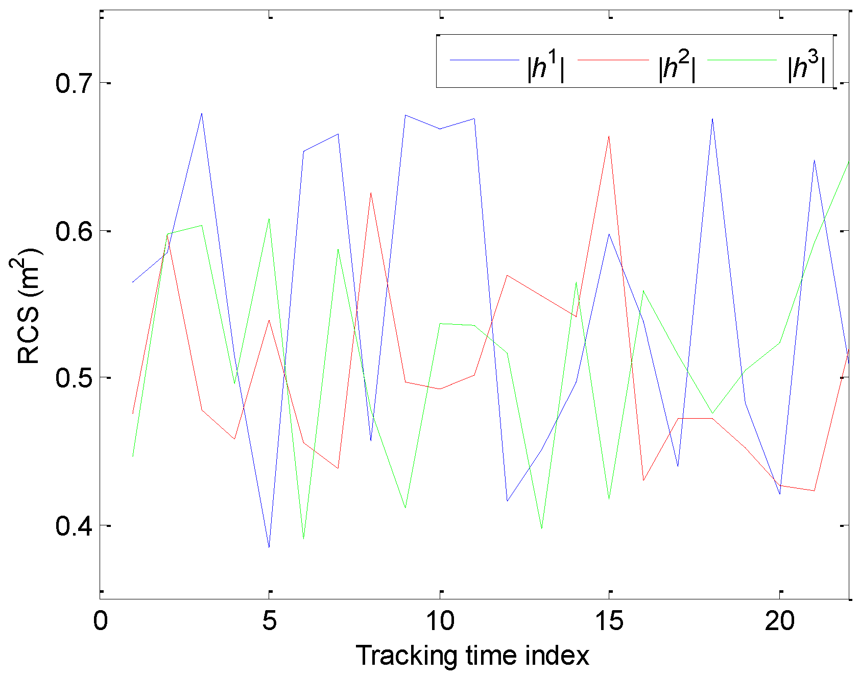
To compare the simulation results fairly and conveniently, it is assumed that all the simulation examples have the same target RCS. The total sampling times of the adaptive sampling algorithm cannot be predetermined in the tracking process. Then, we cannot also determine the number of the observed value of RCS. Herein, we give the changing curve of RCS according to the fixed sampling algorithm with the most sampling times.

Where |hⁱ| is the modulus of target RCS relative to the ith radar in Figure 4.

To proceed, the simulation results and corresponding analysis are presented in the following subsections. In the first three subsections, we all adopt the BFG-UKF for target state estimation. In the last subsection, we compare the tracking effects between BFG-UKF and IMM-UKF.

5.1. Adaptive Sampling Interval

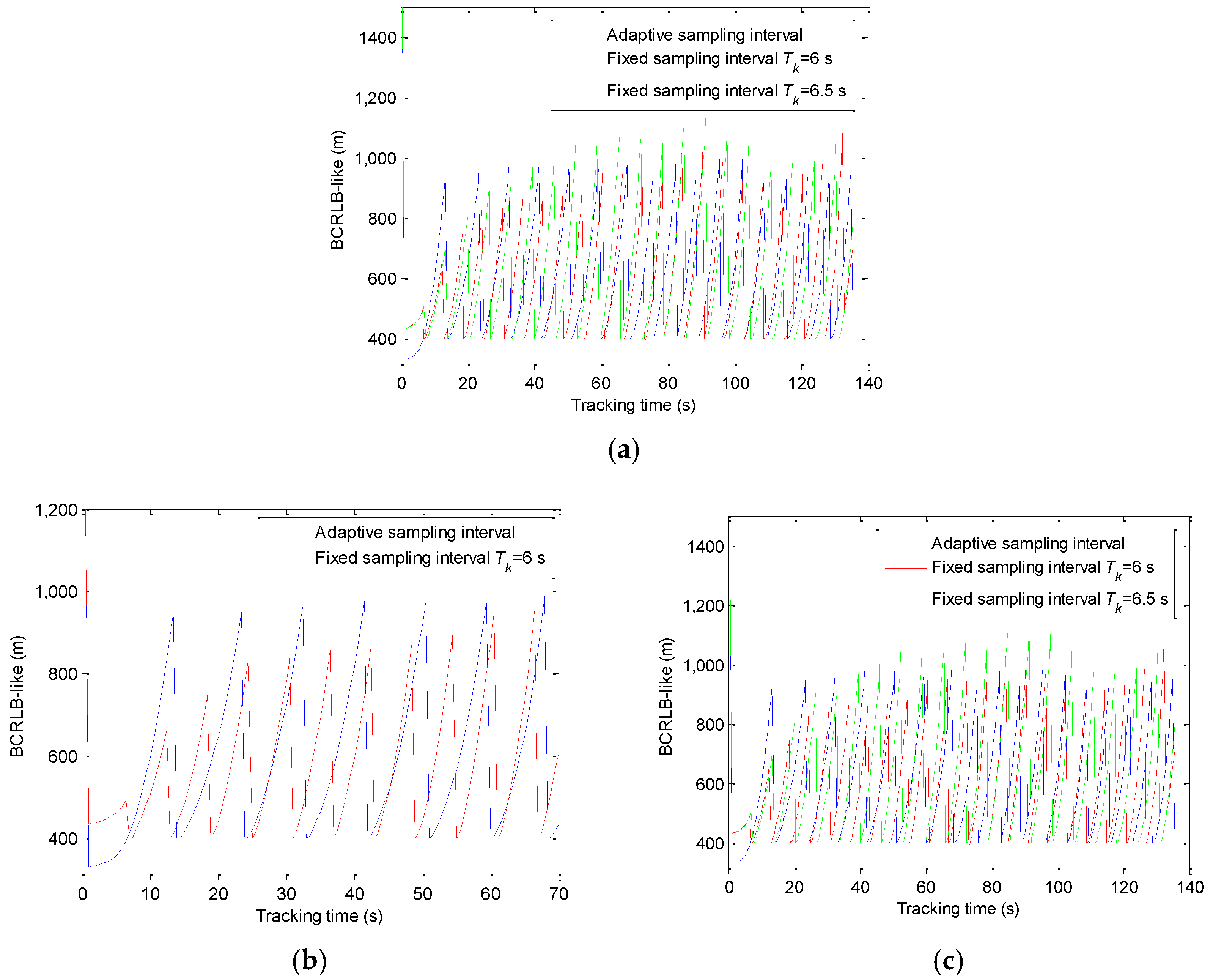
This subsection supports the evaluation of the adaptive sampling algorithm. According to the previous analysis in Section 3.4, the adaptive sampling happens before the power allocation, and we predict the tracking error of the target by F_P(T_k) to determine the sampling interval. The visual simulation results are shown in Figure 5.

The simulation results of the adaptive sampling algorithm and the fixed sampling algorithm are compared in Figure 5. In Figure 5a, besides the adaptive sampling algorithm, we also give two simulation results of the fixed sampling algorithm: T_k = 6 s and T_k = 6.5 s. When T_k = 6.5 s, it can be seen from Figure 5 that the prior CRLB-like value does not satisfy the error threshold constraint in many moments. When T_k = 6 s, the prior CRLB-like basically meets with the error threshold constraint during the whole tracking process. Hence, the fixed sampling interval T_k = 6 s is compared with the adaptive sampling interval detailed in Figure 5b,c. During the whole tracking process, the adaptive sampling times 18 is significantly less than the fixed sampling times 22. In Figure 5b, the adaptive sampling interval is approximately 1.5 to 2 times of the fixed sampling interval T_k = 6 s. The motion state is simple and the velocity is low from 0 to 70 s, so the target tracking error increases slowly, and then the radar system will select a long sampling interval intelligently. In Figure 5c, with the increase of maneuverability and velocity of the target, the length of the adaptive sampling interval is reduced to the length of the fixed sampling interval.

5.2. Optimal Allocation of Power

In this part, when the adaptive sampling algorithm is used for determining the sampling interval, we contrastively analyze the results of optimal power allocation and equal power allocation conditioned on the desired tracking error threshold. By restricting generality, the confidence level is set as α = 0.95 in this simulation.

The power consumption rate is given in Figure 6. The power consumption rate is defined as the ratio of the total transmitted power P_sum and the total power P_total of the radar system. Since the adaptive sampling algorithm is used for the two power allocation methods, it can be seen that they have equal sampling times. Under the condition of the same desired tracking error threshold, the optimal power allocation algorithm can save more power resources than the equal power allocation algorithm, especially between 0 s and 70 s.

P_sum and P_total are the total transmitted power and the total power of the radar system, respectively.

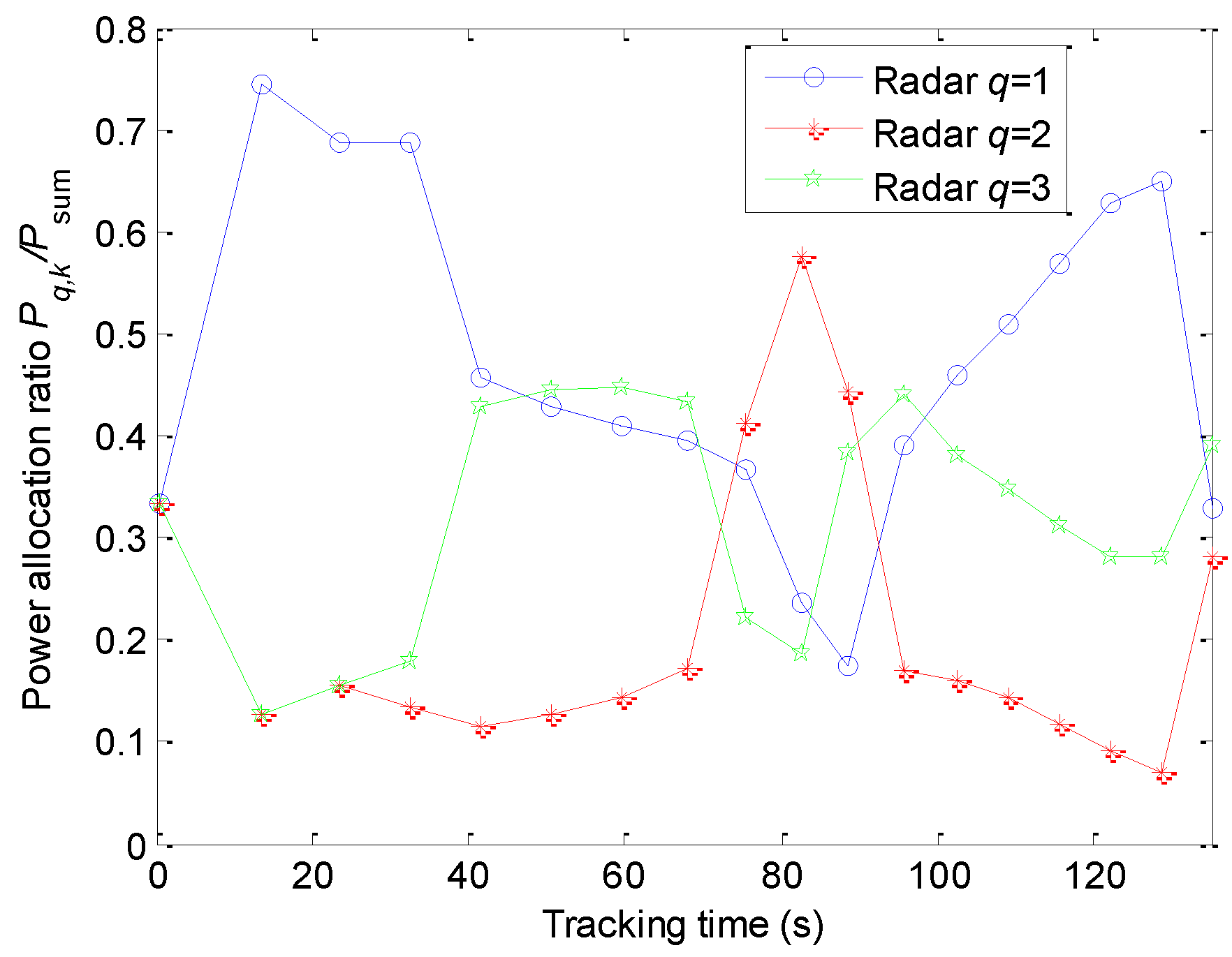
The power allocation algorithm proposed in this case can also intelligently allocate the power among the radars, and the corresponding simulation results are shown in Figure 7. With the moving of the target, the distance between the target and each radar is time-varying. Attributing to the spatially decentralized radars, the azimuth changing rate and target velocity relative to different radars are different. According to Equations (13) and (14), the measurement values of the range, azimuth, and the Doppler shift can all affect the power allocation, i.e., the power allocation is a comprehensive influence of the three elements. Therefore, the power allocation ratios are changed all the time when the target is moved.

P_q,k denotes the transmitted power of the qth radar at the kth sampling instant.

To examine the tracking performance of the proposed power allocation method, we compare the root MSEs (RMSE) of the state vectors of the two power allocation methods. In this case, the position RMSE is defined by the equation below.

$${\mathrm{RMSE}}_k=\sqrt{\frac{1}{N_{\mathrm{MC}}}{\displaystyle \sum _{i=1}^{N_{\mathrm{MC}}}\left[{\left(x_{i,k}-{\hat{x}}_{i,k}\right)}^2+{\left(y_{i,k}-{\hat{y}}_{i,k}\right)}^2\right]}}$$

(63)

where N_MC is the number of Monte Carlo trials and it is set to 100 in this paper. $({\hat{x}}_{i,k},{\hat{y}}_{i,k})$ is the state estimate of the target at the ith trial.

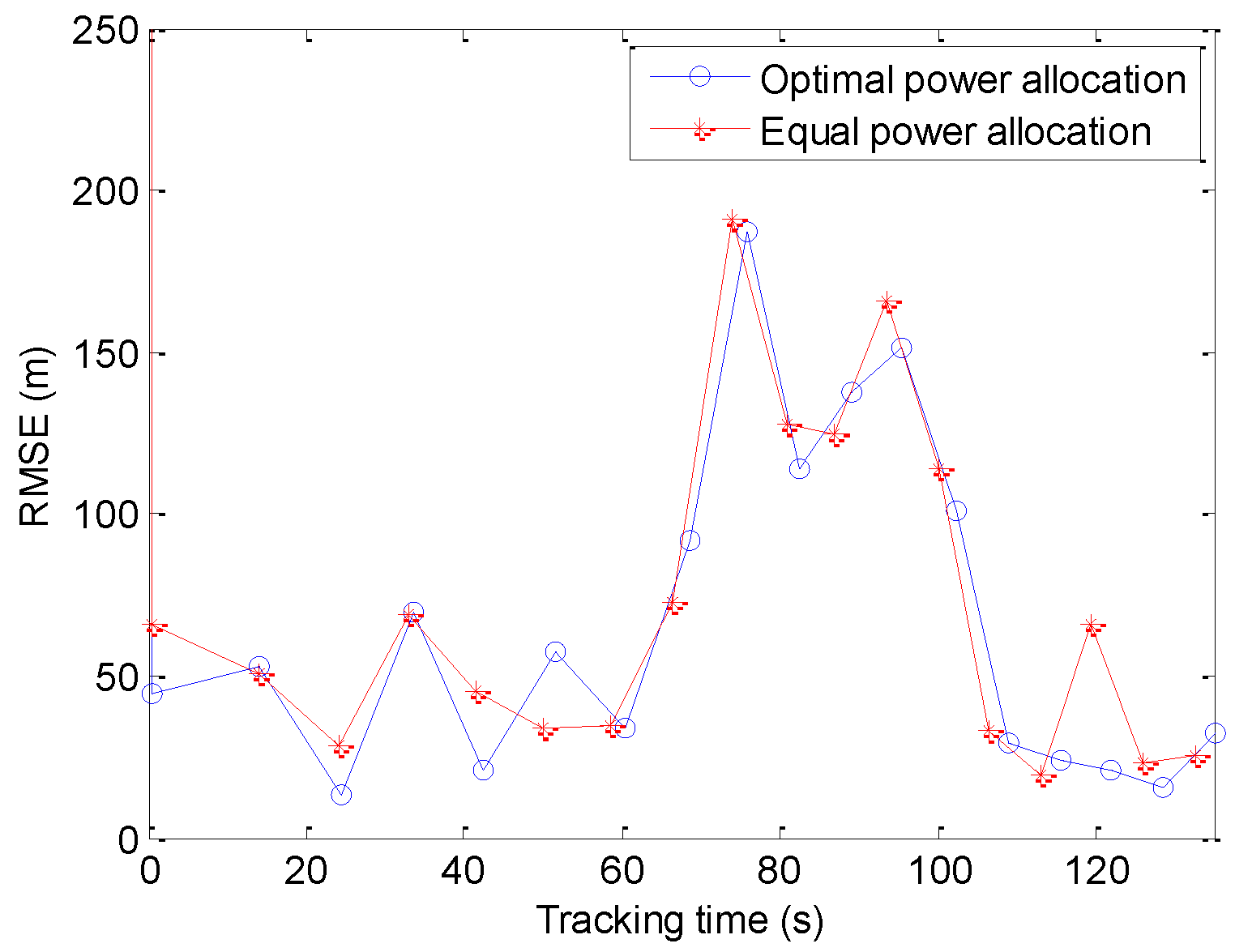
In Figure 8, although the optimal power allocation consumes less transmitted power, its tracking RMSE is not worse than the equal power allocation. This is because the intelligent increase/decrease of the transmitted power of the radars is certainly better than the simultaneous increase/decrease. In addition, the BCRLB-like no longer provides a lower bound on error performance. Meanwhile, to satisfy the specified confidence level of the CCP, the RCS used in the pre-allocation process is less than the RCS used in the state estimation process. Hence, there is no comparability between the RMSE in Figure 8 and the BCRLB-like in Figure 5a.

RMSE is the root mean square error of the target.

5.3. Chance-Constraint Programming

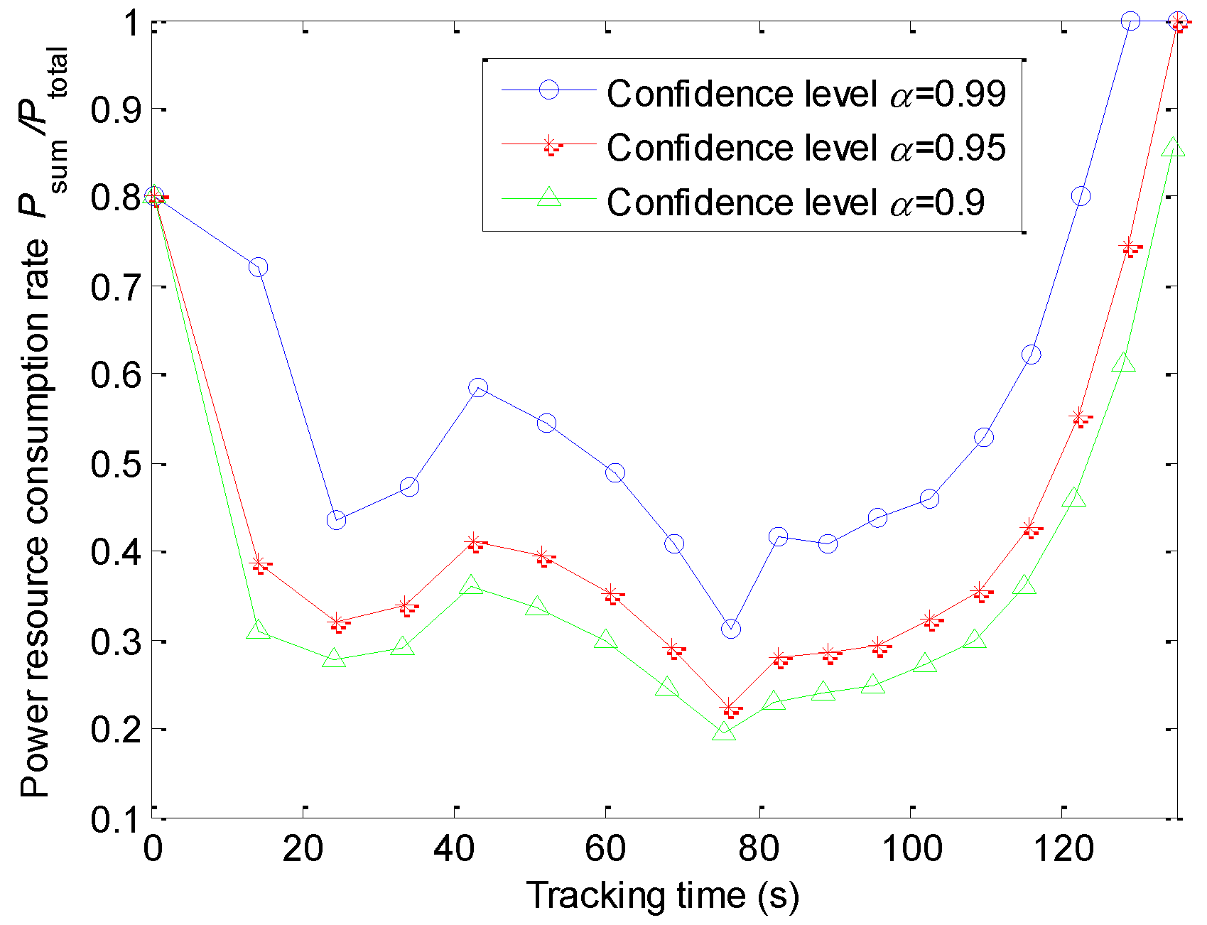
To cope with the randomness of RCS, the CCP is utilized in the simulation. Selecting an appropriate confidence level is crucial. Not only the identity, motion state, and number of the targets, but also the target environments and the amount of radar resource are the factors that impact the confidence level. Considering the previously mentioned factors comprehensively, we specify the confidence level α as 0.99, 0.95, and 0.9 in Figure 9, respectively. As seen from the simulation results, the power consumption is increased with the rise of the confidence levels.

5.4. Target State Estimation with BFG-UKF and IMM-UKF

The regime-dependent motion model is replaced by a single BFG distribution. Consequently, we can use the BFG-UKF to estimate the target state in the previously mentioned three subsections. In this subsection, we compare the RMSE of BFG-UKF and IMM-UKF in Figure 10 and Figure 11.

Where BFG-UKF denotes the UKF combined with BFG.

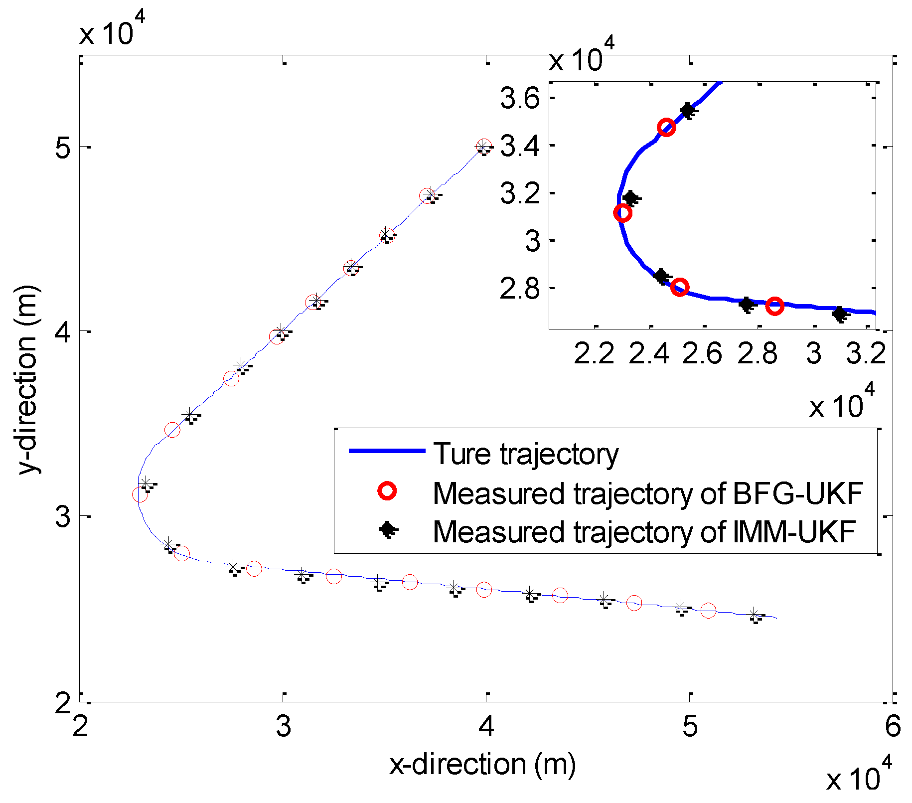
For BFG-UKF (or IMM-UKF) alone in Figure 10, the RMSEs increase with the decrease of the confidence levels. With the decrease of the confidence levels, the power required to satisfy constraints decreases. Then the tracking performance of BFG-UKF (or IMM-UKF) also gets worse. From 0 s to 60 s and 115 s to 135 s, the tracking effects of BFG-UKF and IMM-UKF are nearly the same. However, between 60 s and 115 s, due to the maneuverability of the target, the estimation performance of the two filters both gets worse. By contrast, the estimation performance of BFG-UKF is better than the estimation performance of IMM-UKF. Now, we give an explanation. Although the traditional UKF is not suitable for tracking the maneuvering target, the BFG is introduced to improve the performance of it and a well simulation is obtained. In addition, in the simulation scenario of this paper, the spatial distribution of radars may result in the inexact calculation of the likelihood function, and then the estimation of the target motion mode is influenced in IMM-UKF. Hence, the simulation results in Figure 10 appear.

Meanwhile, Figure 11 verifies our viewpoint again. In addition, we give a local enlarged drawing to emphasize the simulation results. The confidence level is set as α = 0.95 in Figure 11.

The joint resource allocation algorithm of this paper can be extendable to a three-dimensional scenario. In the three-dimensional scenario, the z-coordinate is added into target motion equations. In the measurement model, the elevation angle is added. Hence, compared with the two-dimensional scenario, the BCRLB of the elevation angle is added into Equation (16) in the three-dimensional scenario. The predictive BIM of the elevation angle needs to be calculated. Besides the elevation angle, the other predictive BIMs in Equation (40) also need to be derived again. The filter needs to be changed to a three-dimensional form. The joint resource allocation algorithm of the maneuvering target for a three-dimensional scenario is worthy of studying. The formula derivation and simulation are more complicated. For the length of this paper, the content of the three-dimensional scenario is not involved. We will study this part in the future work.

6. Conclusions

This paper presents a joint adaptive sampling interval and power allocation scheme based on CCP for MTT in a multiple OAR system. Initially, we develop a general approach to replace the MSD of a maneuvering target with a signal BFG distribution. Based on this, the prior CLRB-like is calculated as a criterion for determining the adaptive sampling interval. Meanwhile, the BCRLB-like, which provides a referenced boundary on the tracking error, is exploited as an aid in performing efficient power allocation for MTT. Afterwards, directing at the randomness of target RCS, we package the deterministic resource allocation model as an uncertain model through CCP conditioned on a specified confidence level. Lastly, the resulting optimization problem is solved through HIOA. Simulation results demonstrate the effect of the adaptive sampling algorithm and the power allocation algorithm, the correctness of HIOA for solving the CCP, and the accuracy of BFG-UKF for estimating the maneuvering target state. As can be seen from the derivation, the resource allocation scheme for a single maneuvering target can be easily generalized to a scenario including multiple maneuvering targets, even the distributed OAR case (consists of M₁ transmitting and N₁ receiving radars). In the future work, we will introduce the BFG approximation into the multiple maneuvering target tracking scenario of the distributed OAR.

References

1. Bartee, J.A. Genetic Algorithms as a Tool for Phased Array Radar Design. Master’s Thesis, Naval Postgraduate School, Monterey, CA, USA, 2002. [Google Scholar]
2. Esswein, L.C. Genetic Algorithm Design and Testing of a Random Element 3-D 2.4 GHz Phased Array Transmit Antenna Constructed of Commercial RF Microchips. Master’s Thesis, Naval Postgraduate School, Monterey, CA, USA, 2003. [Google Scholar]
3. Kocaman, İ. Distributed Beamforming in a Swarm UAV Network. Master’s thesis, Naval Postgraduate School, Monterey, CA, USA, 2008. [Google Scholar]
4. Long, W.J.; Ben, D.; Pan, M.H.; Shu, X.R.; Han, Y.M.; Pan, J.B. Opportunistic digital array radar and its technical characteristic analysis. In Proceedings of the IET International Radar Conference, Guilin, China, 20–22 April 2009; pp. 1–4. [Google Scholar]
5. Long, W.J.; Ben, D.; ASIM, B.; Zhang, G. Pattern synthesis optimization of 3-D ODAR based on improved GA using LSFE method. J. Harbin Inst. Technol. (New Ser.) 2011, 18, 96–100. [Google Scholar]
6. Visina, R.; Bar-Shalom, Y.; Willett, P. Multiple-Model Estimators for Tracking Sharply Maneuvering Ground Targets. IEEE Trans. Aerosp. Electron. Syst. 2018, 54, 1–18. [Google Scholar] [CrossRef]
7. Han, B.; Huang, H.Q.; Lei, L.; Huang, C.Q. An Improved IMM Algorithm Based on STSRCKF for Maneuvering Target Tracking. IEEE Access 2019, 7, 57795–57804. [Google Scholar] [CrossRef]
8. Zhang, H.W.; Xie, W.X. Constrained auxiliary particle filtering for bearings-only maneuvering target tracking. J. Syst. Eng. Electron. 2019, 30, 684–695. [Google Scholar]
9. Yu, Y.H. Distributed Multimodel Bernoulli Filters for Maneuvering Target Tracking. IEEE Sens. J. 2018, 18, 5885–5896. [Google Scholar] [CrossRef]
10. Godrich, H.; Petropulu, A.P.; Poor, H.V. Sensor selection in distributed multiple-radar architectures for localization: A knapsack problem formulation. IEEE Trans. Signal Process. 2012, 60, 247–260. [Google Scholar] [CrossRef]
11. Yan, J.K.; Liu, H.W.; Jiu, B.; Chen, B.; Liu, Z.; Bao, Z. Simultaneous multibeam resource allocation scheme for multiple target tracking. IEEE Trans. Signal Process. 2015, 63, 3110–3122. [Google Scholar] [CrossRef]
12. Yan, J.K.; Jiu, B.; Liu, H.W.; Chen, B.; Bao, Z. Prior knowledge-based simultaneous multibeam power allocation algorithm for cognitive multiple targets tracking in clutter. IEEE Trans. Signal Process. 2015, 63, 512–527. [Google Scholar] [CrossRef]
13. Yan, J.K.; Liu, H.W.; Jiu, B.; Liu, Z.; Bao, Z. Joint detection and tracking processing algorithm for target tracking in multiple radar system. IEEE Sens. J. 2015, 15, 6534–6541. [Google Scholar] [CrossRef]
14. Han, Q.H.; Pan, M.H.; Liang, Z.L. Joint power and beam allocation of opportunistic array radar for multiple target tracking in clutter. Digit. Signal Process. 2018, 78, 136–151. [Google Scholar] [CrossRef]
15. Xie, M.C.; Yi, W.; Kirubarajan, T. Joint Node Selection and Power Allocation Strategy for Multitarget Tracking in Decentralized Radar Networks. IEEE Trans. Signal Process. 2018, 66, 729–743. [Google Scholar] [CrossRef]
16. Zheng, N.E.; Sun, Y.; Song, X.Y.; Chen, S. Joint resource allocation scheme for target tracking in distributed MIMO radar systems. J. Syst. Eng. Electron. 2019, 30, 709–719. [Google Scholar]
17. Van Trees, H.L.; Bell, K.L. Bayesian Bounds for Parameter Estimation and Nonlinear Filtering/Tracking; Wiley: New York, NY, USA, 2007. [Google Scholar]
18. Rapoport, I.; Oshman, Y. Recursive Weiss-Weinstein lower bounds for discrete-time nonlinear filtering. In Proceedings of the IEEE Conference Decision Control, Nassau, Bahamas, 14–17 December 2004; pp. 2662–2667. [Google Scholar]
19. Reece, S.; Nicholson, D. Tighter alternatives to the Cramér-Rao lower bound for discrete-time filtering. In Proceedings of the International Conference on Information Fusion, Philadelphia, PA, USA, 25–28 July 2005; pp. 717–722. [Google Scholar]
20. Tichavsky, P.; Muravchik, C.H.; Nehorai, A. Posterior Cramér-Rao bounds for discrete-time nonlinear filtering. IEEE Trans. Signal Process. 1998, 46, 1386–1396. [Google Scholar] [CrossRef] [Green Version]
21. Hernandez, M.; Ristic, B.; Farina, A. A performance bound for manoeuvring target tracking using best-fitting Gaussian distrbutions. In Proceedings of the International Conference on Information Fusion, Philadelphia, PA, USA, 25–28 July 2005; pp. 1–8. [Google Scholar]
22. Hernandez, M.L.; Ristic, B.; Farina, A.; SathYan, T.; Kirubarajan, T. Performance Measure for Markovian Switching Systems using Best-Fitting Gaussian Distributions. IEEE Trans. Aerosp. Electron. Syst. 2008, 44, 724–747. [Google Scholar] [CrossRef]
23. Hernandez, M.; Benavoli, A.; Graziano, A.; Farina, A.; Morelande, M. Performance Measures and MHT for Tracking Move-Stop-Move Targets with MTI Sensors. IEEE Trans. Aerosp. Electron. Syst. 2011, 47, 996–1025. [Google Scholar] [CrossRef]
24. Ristic, B.; Hernandez, M.; Farina, A.; Ong, H.T. Analysis of radar allocation requirements for an IRST aided tracking of anti-ship missiles. In Proceedings of the International Conference on Information Fusion, Florence, Italy, 10–13 July 2006; pp. 1–8. [Google Scholar]
25. Skolnik, M.I. Introduction to Radar System, 3rd ed.; Tata McGraw-Hill Publishing Company Limited: New Delhi, India, 2001; pp. 49–73. [Google Scholar]
26. Liu, B.D. Theory and Practice of Uncertain Programming, 2nd ed.; Springer: Berlin, Germany, 2009. [Google Scholar]
27. Chen, X.; Tharmarasa, R.; Kirubarajan, T. Multitarget multisensor tracking. In Academic Press Library in Signal Processing; Sidiropoulos, N.D., Gini, F., Chellappa, R., Theodoridis, S., Eds.; Academic Press: Cambridge, MA, USA, 2014; Volume 2, pp. 759–812. [Google Scholar]
28. Bar-Shalom, Y.; Li, X.R. Estimation and Tracking: Principles, Techniques and Software; Artech House: Boston, MA, USA, 1993. [Google Scholar]
29. Blackman, S.; Popoli, R. Design and Analysis of Modern Tracking Systems; Artech House: Boston, MA, USA, 1999. [Google Scholar]
30. Bessell, A.; Ristic, B.; Farina, A.; Wang, X.; Arulampalam, M.S. Error performance bounds for tracking a manoeuvring target. In Proceedings of the International Conference on Information Fusion, Cairns, Australia, 8–11 July 2003; pp. 903–910. [Google Scholar]
31. Van Trees, H.L. Detection, Estimation, Modulation Theory Part III; Wiley: New York, NY, USA, 1971. [Google Scholar]
32. Van Trees, H.L. Optimum Array Processing: Detection, Estimation, Modulation Theory IV; Wiley: New York, NY, USA, 2001. [Google Scholar]
33. Godrich, H.; Petropulu, A.P.; Poor, H.V. Power allocation strategies for target localization in distributed multiple-radar architecture. IEEE Trans. Signal Process. 2011, 59, 3226–3240. [Google Scholar] [CrossRef]
34. Glass, J.D.; Smith, L.D. MIMO radar resource allocation using posterior Cramér-Rao lower bounds. In Proceedings of the IEEE Aerospace Conference, Big Sky, MT, USA, 5–12 March 2011; pp. 1–9. [Google Scholar]
35. Charnes, A.; Cooper, W.W. Chance-constrained programming. Manag. Sci. 1959, 6, 73–79. [Google Scholar] [CrossRef]
36. Gustafsson, F.; Gunnarsson, F.; Bergman, N.; Forssell, U.; Jansson, J.; Karlsson, R.; Nordlund, P.J. Particle Filters for Positioning, Navigation, and Tracking. IEEE Trans. Signal Process. 2002, 50, 425–437. [Google Scholar] [CrossRef] [Green Version]
37. Míguez, J. Analysis of selection methods for cost-reference particle filtering with applications to maneuvering target tracking and dynamic optimization. Digit. Signal Process. 2007, 17, 787–807. [Google Scholar] [CrossRef]
38. Zaitouny, A.; Stemler, T.; Judd, K. Tracking rigid bodies using only position data: A shadowing filter approach based on newtonian dynamics. Digit. Signal Process. 2017, 67, 81–90. [Google Scholar] [CrossRef]
39. Zaitouny, A.; Stemler, T.; Algar, S.D. Optimal Shadowing Filter for a Positioning and Tracking Methodology with Limited Information. Sensors 2019, 19, 931. [Google Scholar] [CrossRef] [PubMed] [Green Version]
40. Challa, S.; Morelande, M.R.; Mušcki, D.; Evans, R.J. Fundamentals of Object Tracking; Cambridge University Press: New York, NY, USA, 2011. [Google Scholar]
41. Rong Li, X.; Jilkov, V.P. Survey of maneuvering target tracking. Part V. Multiple-model methods. IEEE Trans. Aerosp. Electron. Syst. 2005, 41, 1255–1321. [Google Scholar] [CrossRef]
42. Babu, V.S.; Shankar, M.R.; Majumdar, S.; Koteswara Rao, S. IMM-unscented Kalman filter based tracking of maneuvering targets using active sonar measurements. In Proceedings of the International Conference on Communications and Signal Processing, Calicut, India, 10–12 February 2011; pp. 126–130. [Google Scholar]
43. Wang, X.B.; Pang, X.S.; Wang, D.S. Sequential algorithm for extended H∞ filter-based target tracking in wireless sensor networks. In Proceedings of the Chinese Control Conference, Hangzhou, China, 28–30 July 2015; pp. 7721–7725. [Google Scholar]
Figure 1. Centralized fusion architecture.
Sensors 20 00981 g001
Figure 2. Block diagram of resource management for maneuvering target tracking (MTT).
Sensors 20 00981 g002
Figure 3. Target tracking scenario.
Sensors 20 00981 g003
Figure 4. The radar cross section (RCS) of the target relative to different radars.
Sensors 20 00981 g004
Figure 5. The comparison between the adaptive sampling interval and the fixed sampling interval with different tracking time (a) 0–135 s; (b) 0–70 s; (c) 70–135 s.
Sensors 20 00981 g005
Figure 6. Power resource consumption rate.
Sensors 20 00981 g006
Figure 7. Power allocation ratio.
Sensors 20 00981 g007
Figure 8. The root mean square error (RMSE) of optimal and equal power allocation.
Sensors 20 00981 g008
Figure 9. Power consumption of different confidence levels.
Sensors 20 00981 g009
Figure 10. RMSE of different filters.
Sensors 20 00981 g010
Figure 11. The true and measured trajectories of the maneuvering target.
Sensors 20 00981 g011