A Crop Canopy Localization Method Based on Ultrasonic Ranging and Iterative Self-Organizing Data Analysis Technique Algorithm

Abstract
:1. Introduction
2. Materials and Methods
2.1. Experimental Apparatus
2.2. Data Processing Method
2.2.1. Basic Principle
2.2.2. Split and Merge
2.2.3. Algorithm Procedures
2.2.4. Clustering Effect Test
3. Results and Discussion
3.1. Algorithm Verification
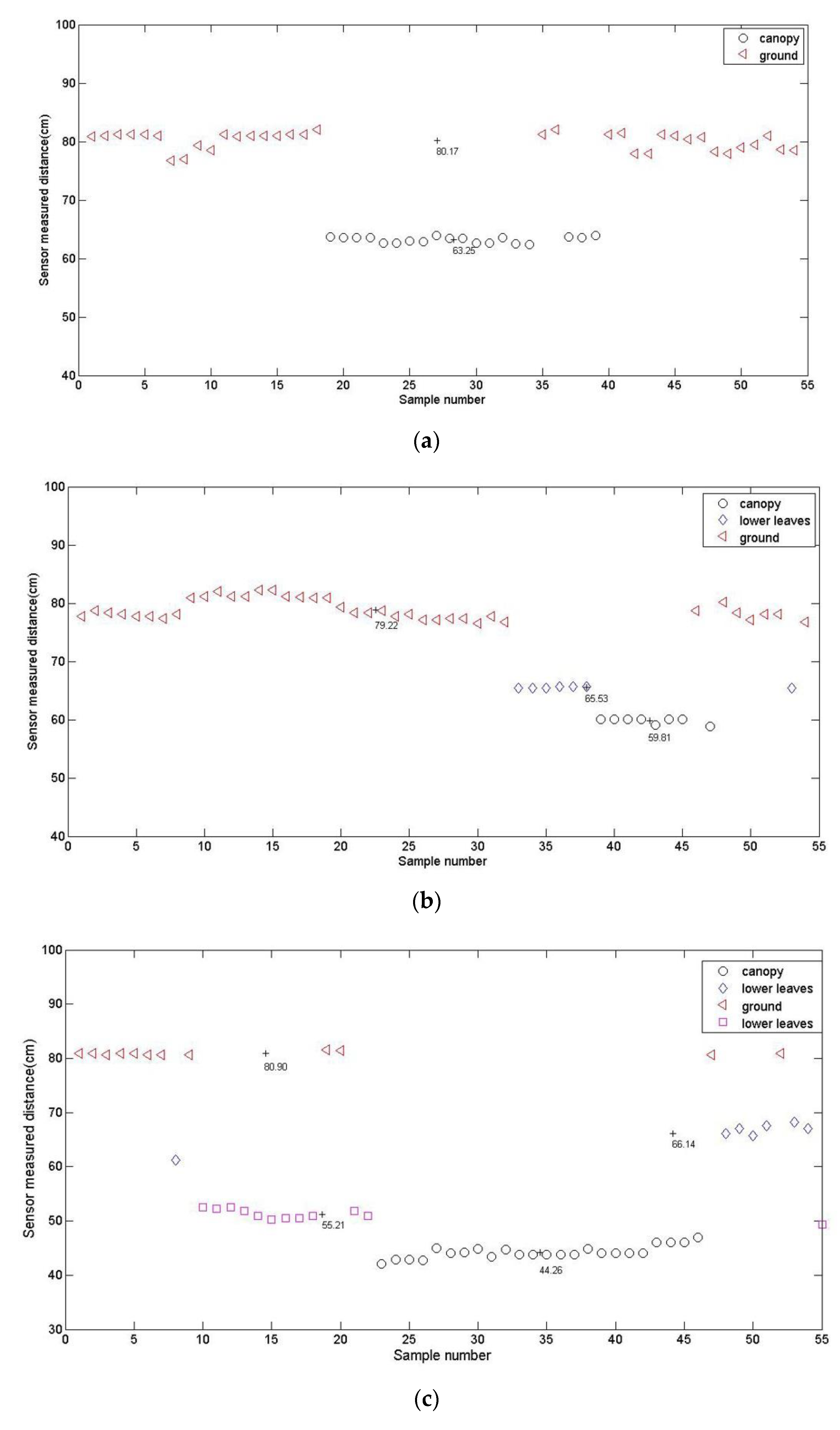
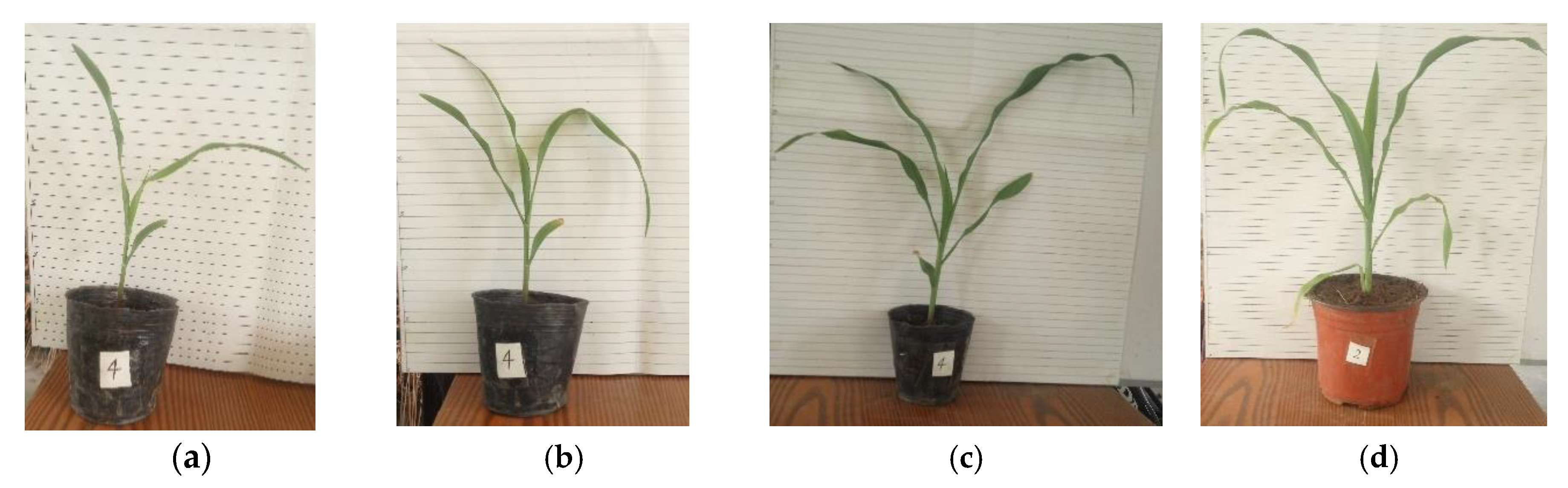
3.2. Influence of Plant Growth Stage on Calculation Accuracy
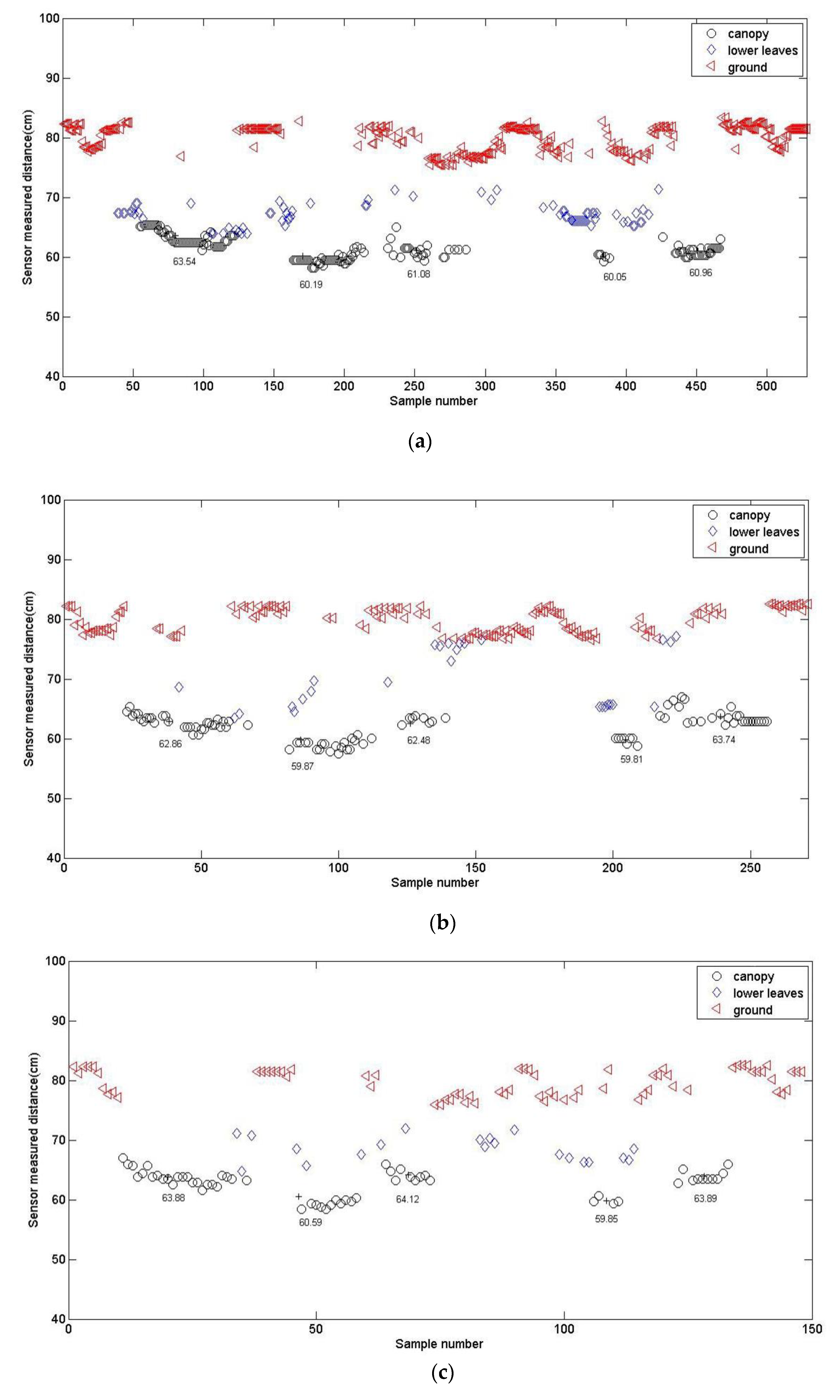
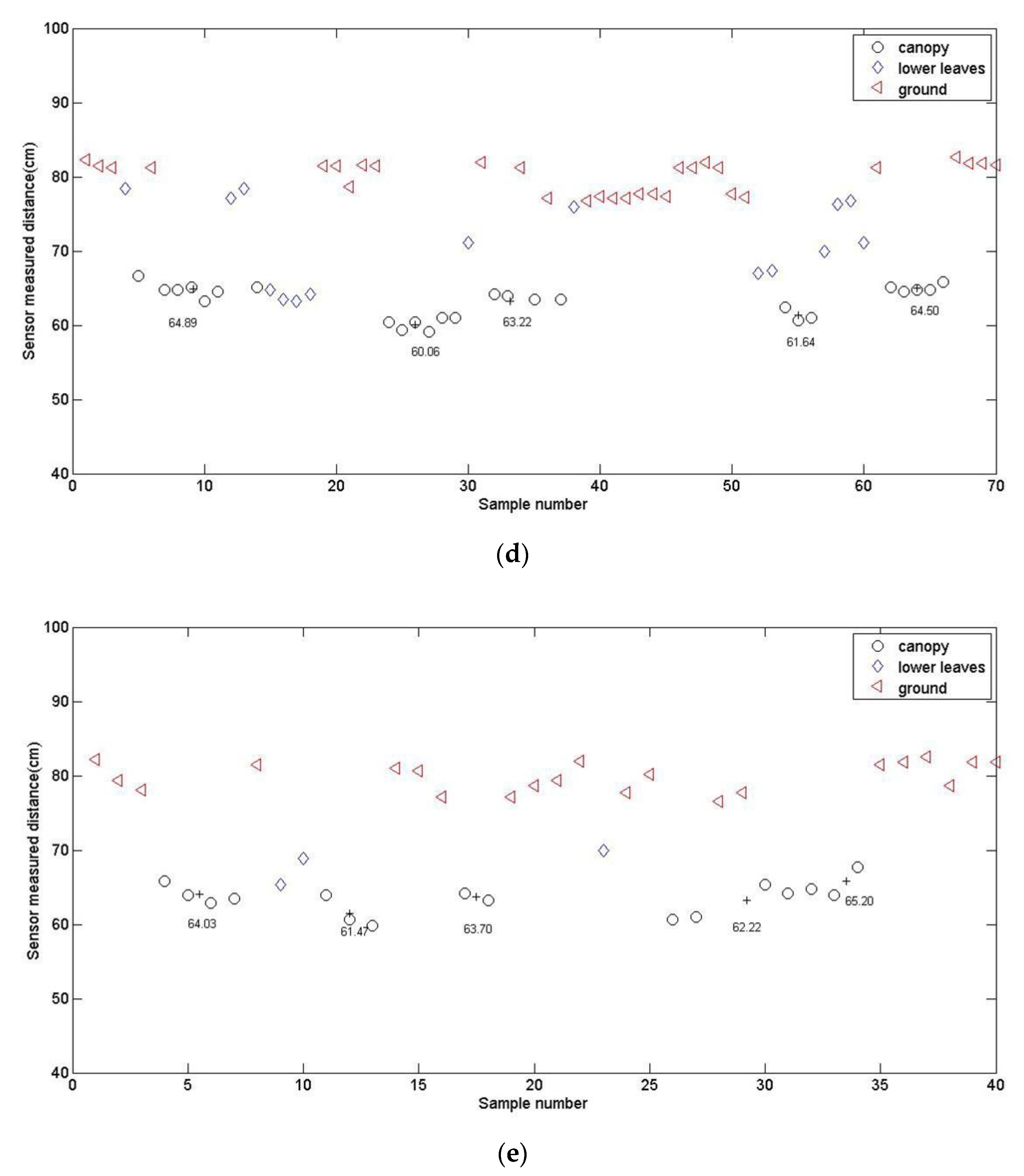
3.3. Influence of Sensor Moving Speed on Calculation Accuracy
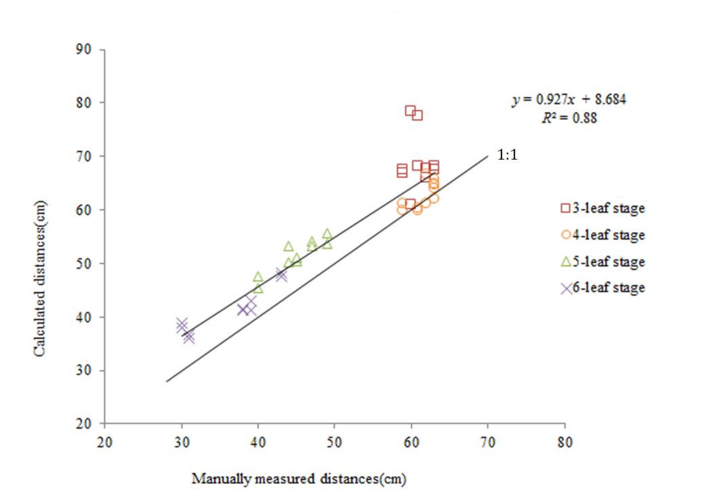
3.4. Correlation between Calculated Values and Manually Measured Values
4. Conclusions
Author Contributions
Funding
Conflicts of Interest
References
- Qi, L.; Fu, Z. Experimental study on spray deposition uniformity. Trans. Csae 1999, 15, 113–117. [Google Scholar]
- Chen, Z.; Wu, C.; Yang, X. Spray distribution uniformity of boom spraying. J. Jiangsu Univ. 2008, 29, 465–468. [Google Scholar]
- Jeon, H.; Womac, A.; Gunn, J. Sprayer boom dynamic effects on application uniformity. Trans. ASAE 2004, 47, 647–658. [Google Scholar] [CrossRef]
- Andreas, H.; Hans, O.; Hartje, S. A novel method for testing automatic systems for controlling the spray boom height. Biosyst. Eng. 2018, 174, 115–125. [Google Scholar]
- Ramon, H.; Missotten, B.; Baerdemaeker, J. Spray boom motions and spray distribution: Part 2, Experimental validation of the mathematical relation and simulation results. J. Agri. Eng. Res. 1997, 66, 31–39. [Google Scholar] [CrossRef]
- Paolo, B.; Emilio, G. Field-crop-sprayer potential drift measured using test bench: Effects of boom height and nozzle type. Biosyst. Eng. 2017, 154, 3–13. [Google Scholar]
- Cui, L.; Xue, X.; Ding, S. Analysis and test of dynamic characteristic of large spray in boom and pendulum suspension damping system. Trans. CSAE 2017, 33, 61–68. [Google Scholar]
- Qiu, B.; Yan, R.; Ma, J. Research progress analysis of variable rate sprayer technology. Trans. CSAM 2015, 46, 59–72. [Google Scholar]
- Dionisio, A.; Martin, W.; Roland, G. An Ultrasonic System for Weed Detection in Cereal Crops. Sensors 2012, 12, 17343–17357. [Google Scholar]
- Thomas, F.; Felix, R.; Michal, W. Assessment of forage mass from grassland swards by height measurement using an ultrasonic sensor. Comput. Electron. Agric. 2011, 79, 142–152. [Google Scholar]
- Shrestha, D.S.; Steward, B.L.; Birrell, S.J. Corn plant height estimation using two sensing systems. In Proceedings of the 2002 ASAE Annual International Meeting/ CIGR XVth World Congress, Chicago, IL, USA, 28–31 July 2002; p. 021197. [Google Scholar]
- Kataoka, T.; Okamoto, H.; Kaneko, T.; Hata, S. Performance of corn height sensing using ultrasonic sensor and laser beam sensor. In Proceedings of the 2002 ASAE Annual International Meeting/ CIGR XVth World Congress, Chicago, IL, USA, 28–31 July 2002; p. 021184. [Google Scholar]
- Chang, Y.K.; Zaman, Q.U.; Rehman, T.U.; Farooque, A.A.; Esau, T.; Jameel, M.W. A real-time ultrasonic system to measure wild blueberry plant height during harvesting. Biosyst. Eng. 2017, 157, 35–44. [Google Scholar] [CrossRef]
- Liu, X.; Li, Y.; Li, M. Design and test of smart-targeting spraying system on boom sprayer. Trans. CSAM 2016, 47, 37–44. [Google Scholar]
- Wei, X.; Shao, J.; Miao, D. Online control system of spray boom height and balance. Trans. CSAM 2015, 46, 66–71. [Google Scholar]
- Wang, S.; Zhao, C.; Wang, X. Design and experiments on boom height adjusting system. J. Agri. Mech. Res. 2014, 36, 161–164. [Google Scholar]
- Jin, X.; Zhang, H.; Zhou, Y. Agricultural land gradation based on the fuzzy ISODATA clustering method. Trans. CSAE 2008, 24, 82–85. [Google Scholar]
- Park, H.; Jun, C. A simple and fast algorithm for K-means clustering. Expert Syst. Appl. 2009, 36, 3336–3341. [Google Scholar] [CrossRef]
- Jin, H.; Shi, D.; Chen, Z. Evaluation indicators of cultivated layer soil quality for red soil slope farmland based on cluster and PCA analysis. Trans. CSAE 2018, 34, 155–164. [Google Scholar]
- Pan, R.; Liu, J.; Song, D. Agricultural land classification based on fuzzy comprehensive analysis. Trans. CSAE 2014, 30, 257–265. [Google Scholar]
- Zhao, R.; Huang, X.; Zhong, T.; Xu, H. Application of clustering analysis to land use zoning of coastal region in Jiangsu Province. Trans. CSAE 2010, 26, 310–314. [Google Scholar]
- Bezdek, J.C. A physical interpretation of fuzzy ISODATA. IEEE Trans. SMC 1976, 6, 387–390. [Google Scholar]


| Growth Stage | Number of Clusters | Cluster Center Value (cm) | |||
|---|---|---|---|---|---|
| 3-leaf stage | 2 | 80.17 | 63.25 | ||
| 4-leaf stage | 3 | 79.22 | 65.53 | 59.81 | |
| 5-leaf stage | 4 | 80.90 | 66.14 | 51.21 | 44.26 |
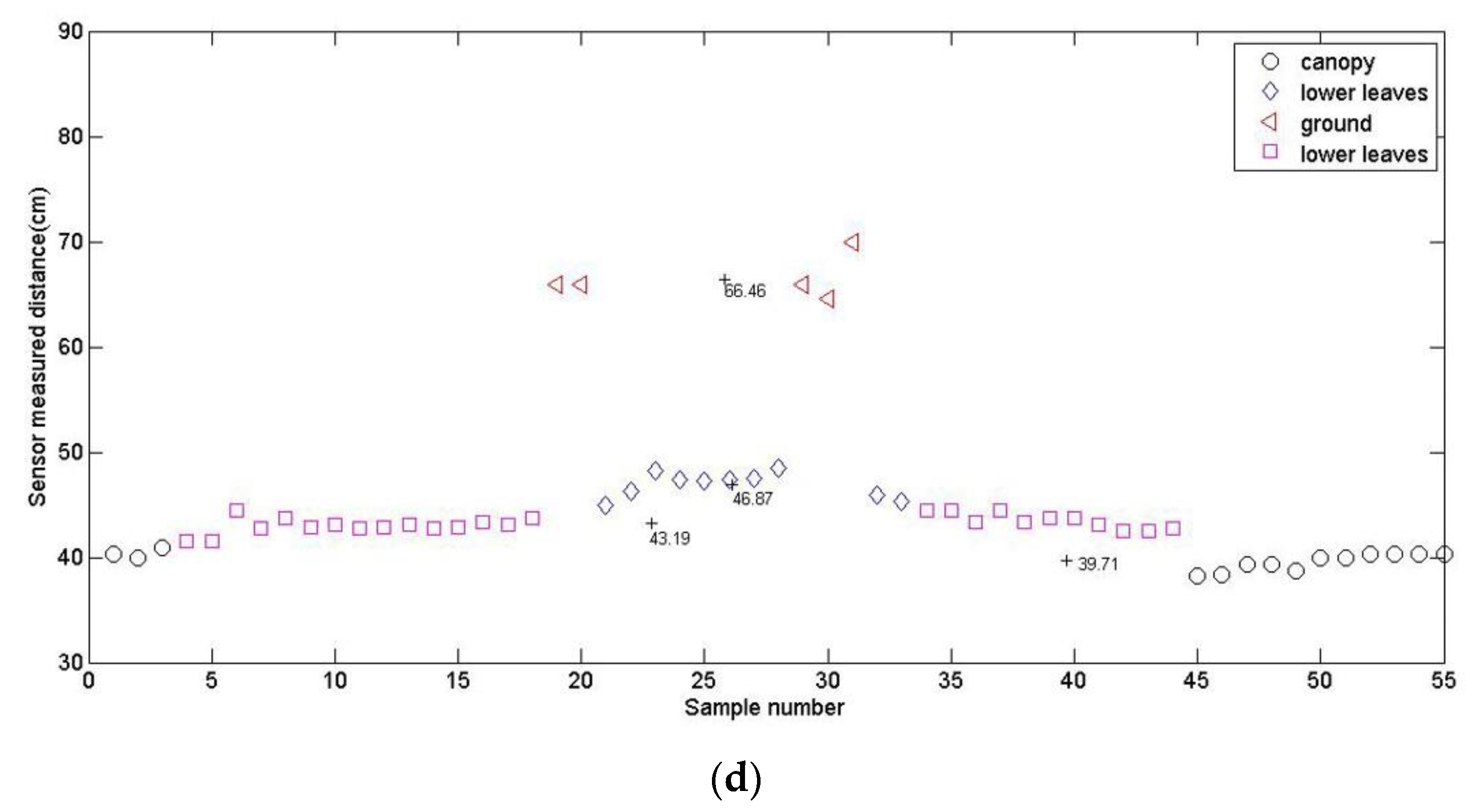
| 6-leaf stage | 4 | 66.46 | 46.87 | 43.19 | 39.71 |
| Growth Stage | Manually Measured Value (cm) | Fuzzy ISODATA (cm) | K-Means Clustering (cm) | Mean (cm) | Median (cm) |
|---|---|---|---|---|---|
| 3-leaf stage | 60 | 63.25 | 63.65 | 74.22 | 78.6 |
| 4-leaf stage | 57 | 59.81 | 65.52 | 74.33 | 77.70 |
| 5-leaf stage | 46 | 44.26 | 43.89 | 55.05 | 50.75 |
| 6-leaf stage | 38 | 39.71 | 42.00 | 45.18 | 43.1 |
| Growth Stage | Calculated Value (cm) | Manually Measured Value (cm) | Absolute Error (cm) |
|---|---|---|---|
| 3-leaf stage | 63.25 | 60 | 3.25 |
| 4-leaf stage | 59.81 | 57 | 2.81 |
| 5-leaf stage | 44.26 | 46 | 1.74 |
| 6-leaf stage | 39.71 | 38 | 1.71 |
| Plant Number | Manually Measured Value (cm) | Calculated Value at Different Speed (cm) | ||||
|---|---|---|---|---|---|---|
| 0.5 km/h | 1 km/h | 2 km/h | 4 km/h | 6 km/h | ||
| Plant no. 1 | 61 | 63.54 | 62.86 | 63.88 | 64.89 | 64.03 |
| Plant no. 2 | 59 | 60.19 | 59.87 | 60.59 | 60.06 | 61.47 |
| Plant no. 3 | 60 | 61.08 | 62.48 | 64.12 | 63.22 | 63.7 |
| Plant no. 4 | 57 | 60.05 | 59.81 | 59.85 | 61.64 | 62.22 |
| Plant no. 5 | 61 | 60.96 | 63.74 | 63.89 | 64.5 | 65.2 |
| Mean values | 59.6 | 61.164 | 61.752 | 62.466 | 62.862 | 63.324 |
| Absolute error | 1.564 | 2.152 | 2.866 | 3.262 | 3.724 | |
| t value | 0.15 | 0.09 | 0.04 | 0.02 | 0.01 | |
| Value | V = 0.5 km/h | V = 1 km/h | V = 2 km/h | V = 4 km/h | V = 6 km/h |
|---|---|---|---|---|---|
| h | 0 | 0 | 0 | 0 | 0 |
| p | 0.5 | 0.3481 | 0.1853 | 0.2078 | 0.5 |
| Source | Sum of Squares of Deviation | Degree of Freedom | Mean Squares of Deviation | F Value | Significance |
|---|---|---|---|---|---|
| Groups | 14.91 | 4 | 3.73 | 3.16 | * |
| Error | 23.64 | 20 | 1.18 | ||
| Total | 38.55 | 24 |
© 2020 by the authors. Licensee MDPI, Basel, Switzerland. This article is an open access article distributed under the terms and conditions of the Creative Commons Attribution (CC BY) license (http://creativecommons.org/licenses/by/4.0/).
Share and Cite
Li, F.; Bai, X.; Li, Y. A Crop Canopy Localization Method Based on Ultrasonic Ranging and Iterative Self-Organizing Data Analysis Technique Algorithm. Sensors 2020, 20, 818. https://doi.org/10.3390/s20030818
Li F, Bai X, Li Y. A Crop Canopy Localization Method Based on Ultrasonic Ranging and Iterative Self-Organizing Data Analysis Technique Algorithm. Sensors. 2020; 20(3):818. https://doi.org/10.3390/s20030818
Chicago/Turabian StyleLi, Fang, Xiaohu Bai, and Yongkui Li. 2020. "A Crop Canopy Localization Method Based on Ultrasonic Ranging and Iterative Self-Organizing Data Analysis Technique Algorithm" Sensors 20, no. 3: 818. https://doi.org/10.3390/s20030818
APA StyleLi, F., Bai, X., & Li, Y. (2020). A Crop Canopy Localization Method Based on Ultrasonic Ranging and Iterative Self-Organizing Data Analysis Technique Algorithm. Sensors, 20(3), 818. https://doi.org/10.3390/s20030818