ISSD: Improved SSD for Insulator and Spacer Online Detection Based on UAV System


Abstract
1. Introduction
- (1)
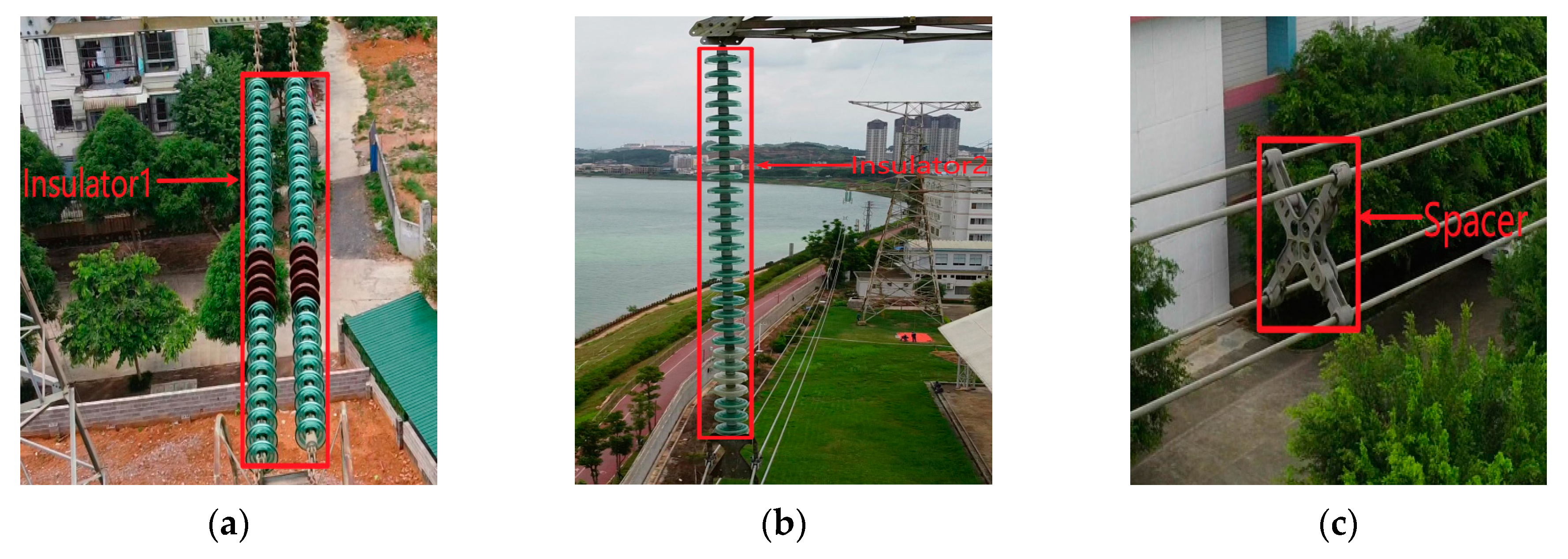
- A new dataset named ISD-dataset is constructed, which can be used for insulator and spacer detection through aerial images. The ISD-dataset contains three types of objects, i.e., Insulator1, Insulator2, and spacer, which allows effectively testing the performance of the object detection algorithm for UAV power inspection.
- (2)
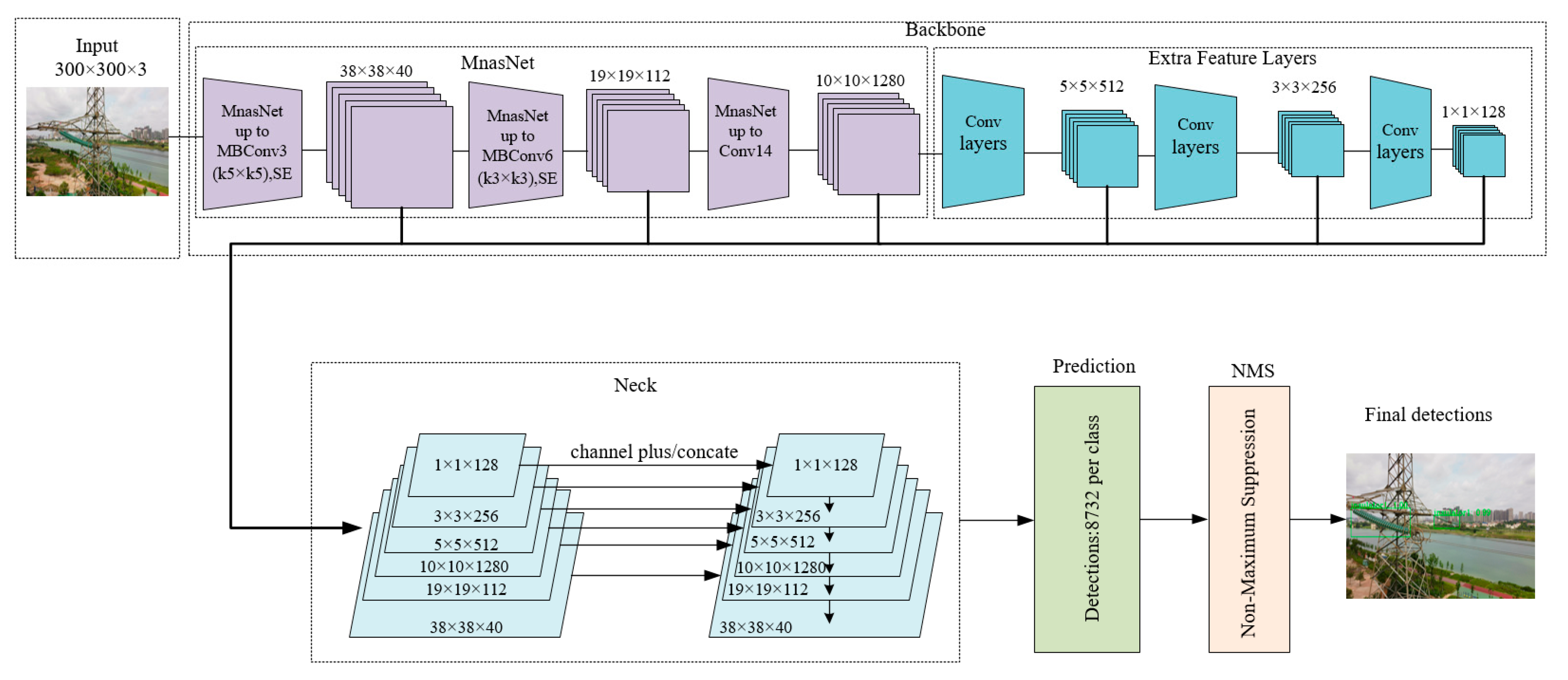
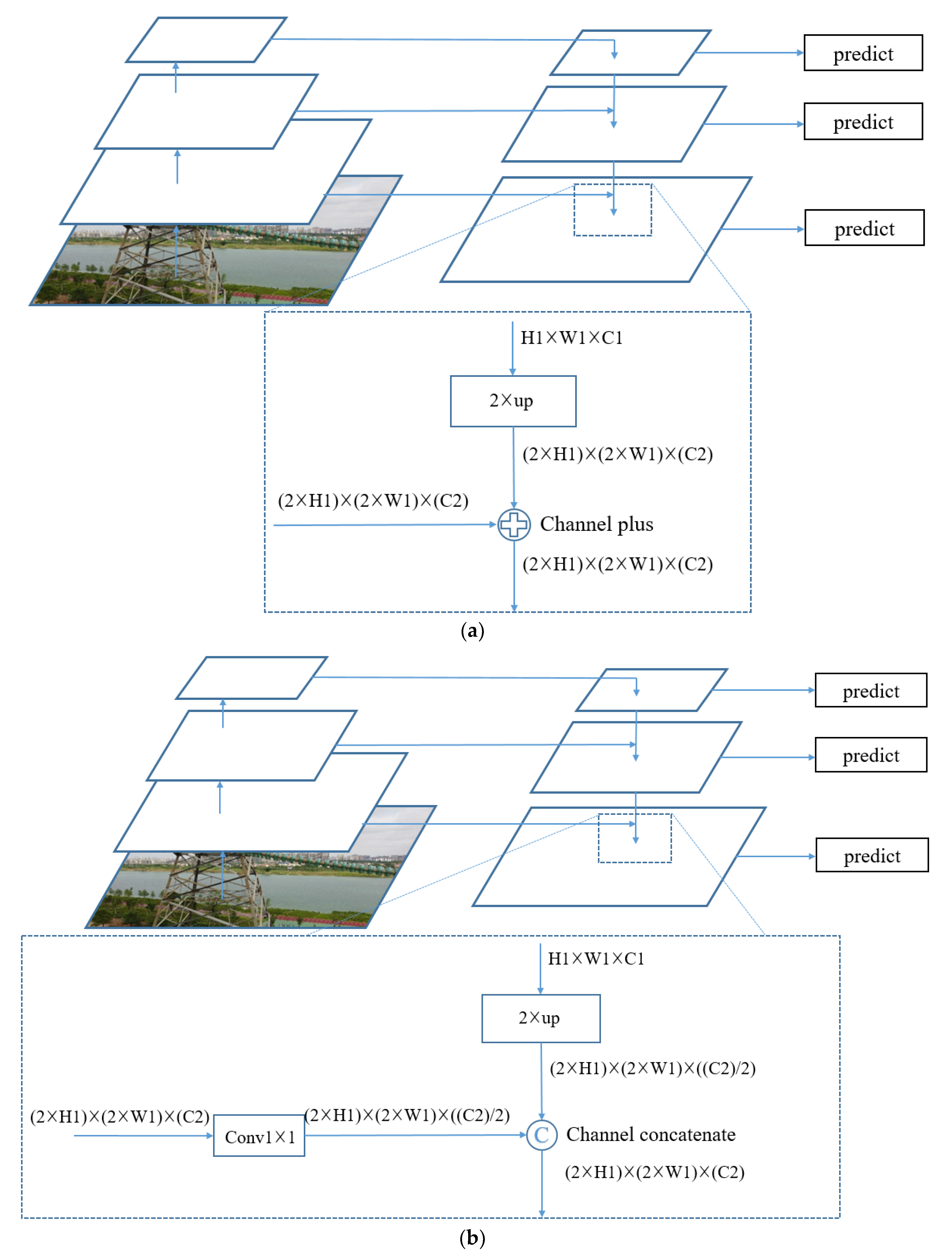
- An improved SSD algorithm for UAV online detection of insulator and spacer is proposed. The improved algorithm uses a lightweight network, i.e., MnasNet, as the feature extraction network, which improves the feature extraction capability and reduces the amount of calculation and model size. This network can generate feature maps with rich features more quickly. Then, two multiscale feature fusion methods, i.e., Channel plus and Channel concatenate, are used to fuse low-level features and high-level features to improve the detection accuracy. The proposed algorithm is superior to previous algorithms in terms of accuracy and speed.
- (3)
- We test the performance of the proposed algorithm, faster R-CNN, R-FCN, and SSD on the ISD-dataset. The comparison of experimental results proves that the proposed algorithm has the advantages of being a small model with high accuracy and fast detection speed. The test results on TX2 show that the proposed algorithm is more suitable for deployment on mobile devices (e.g., TX2). The online detection results of video can be found at https://github.com/PromiseXuan/Insulator-detection.
2. Related Works
2.1. Faster R-CNN
2.2. R-FCN
2.3. SSD
3. Proposed Method
3.1. Backbone
3.2. Neck
3.3. Loss Function and Optimization
4. Experiments
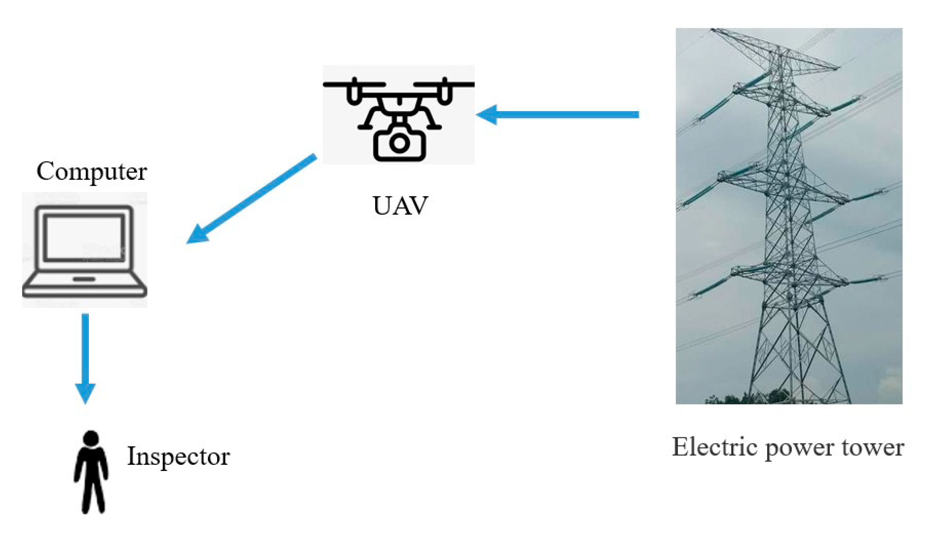
4.1. Offline Detection versus Online Detection
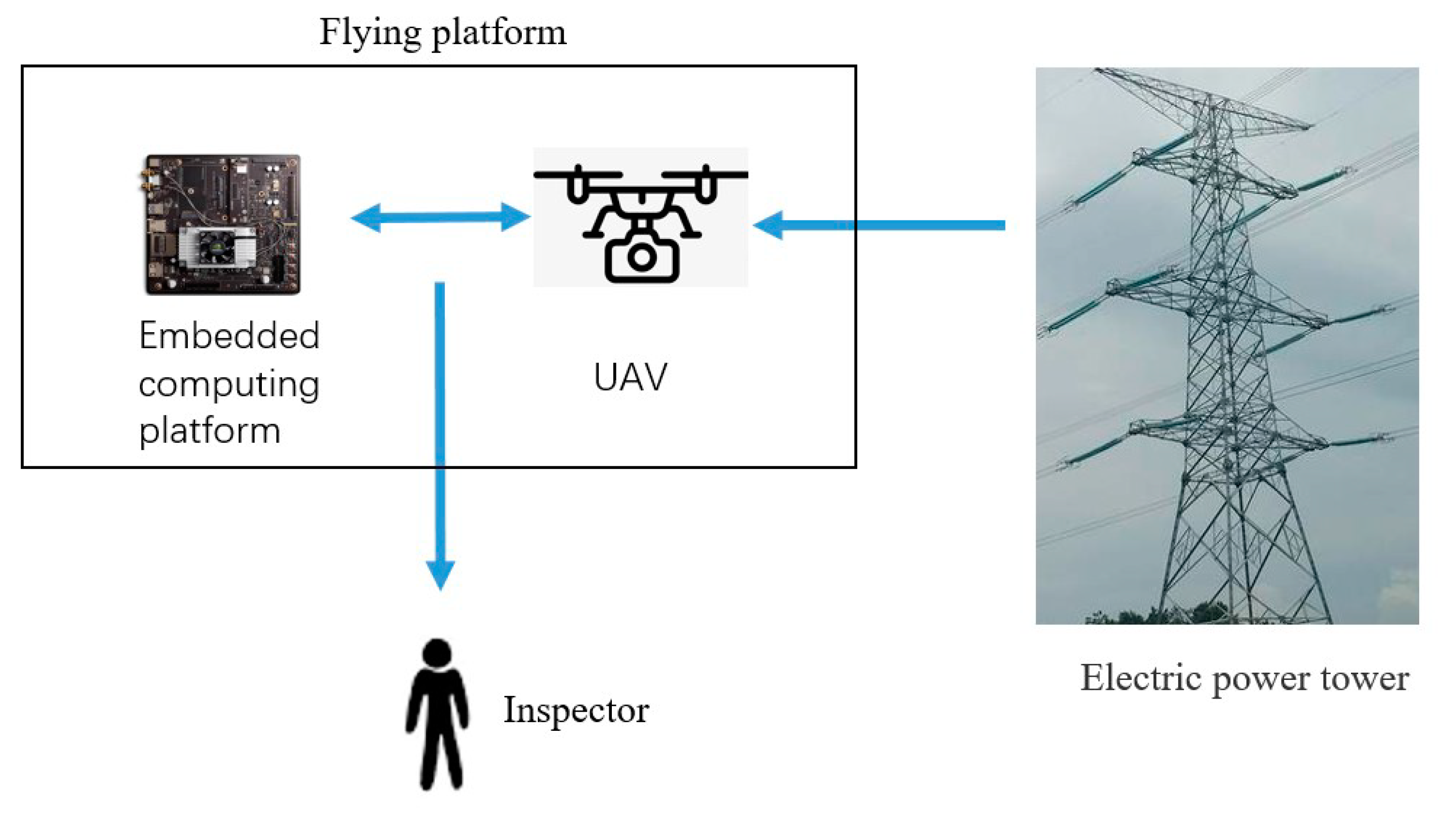
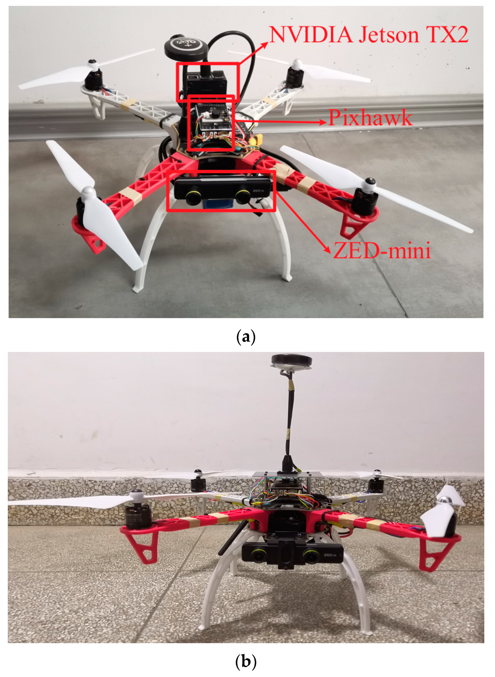
4.2. UAV Platform
4.3. Dataset
4.4. Experimental Setup
4.5. Experimental Results and Analysis
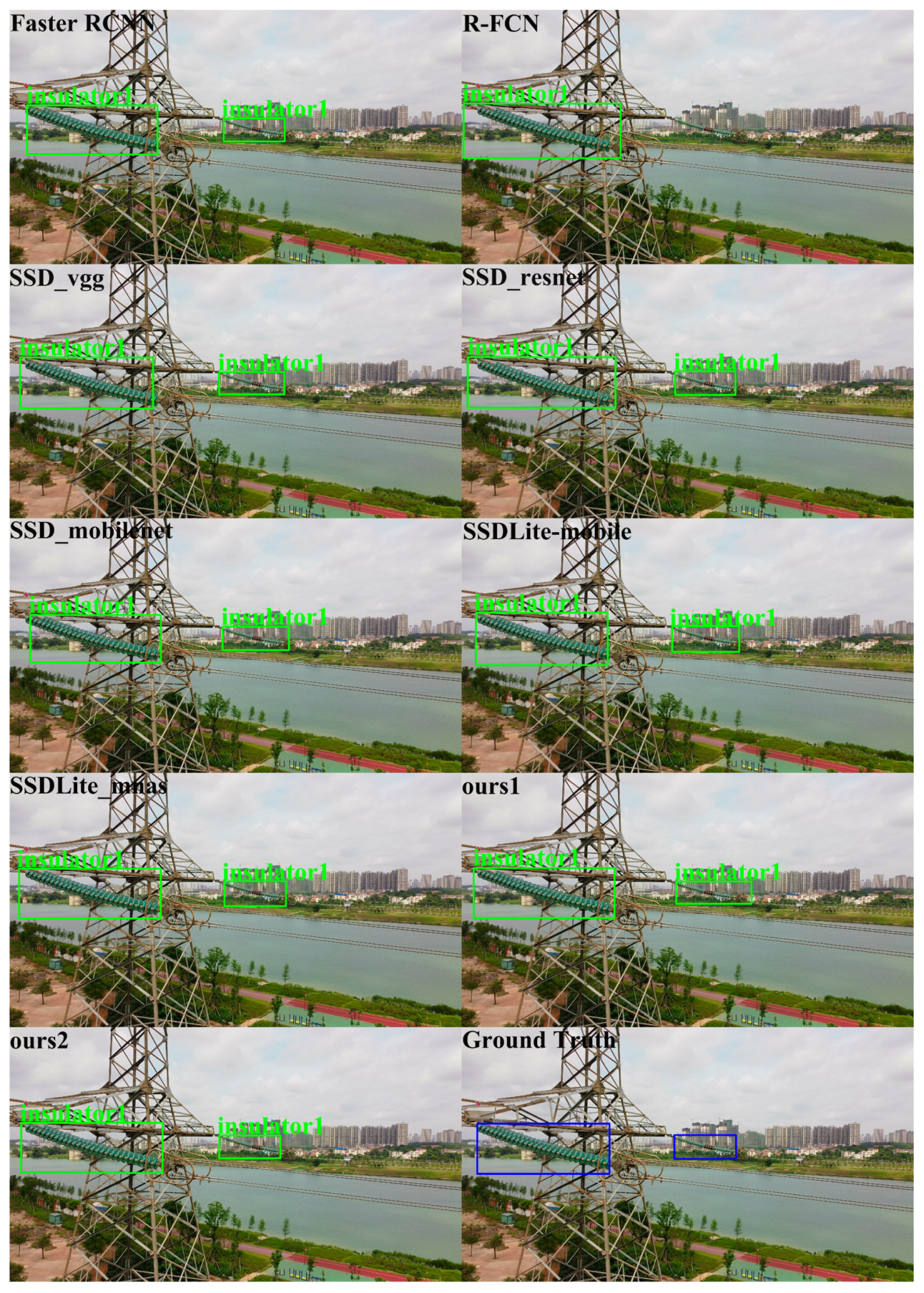
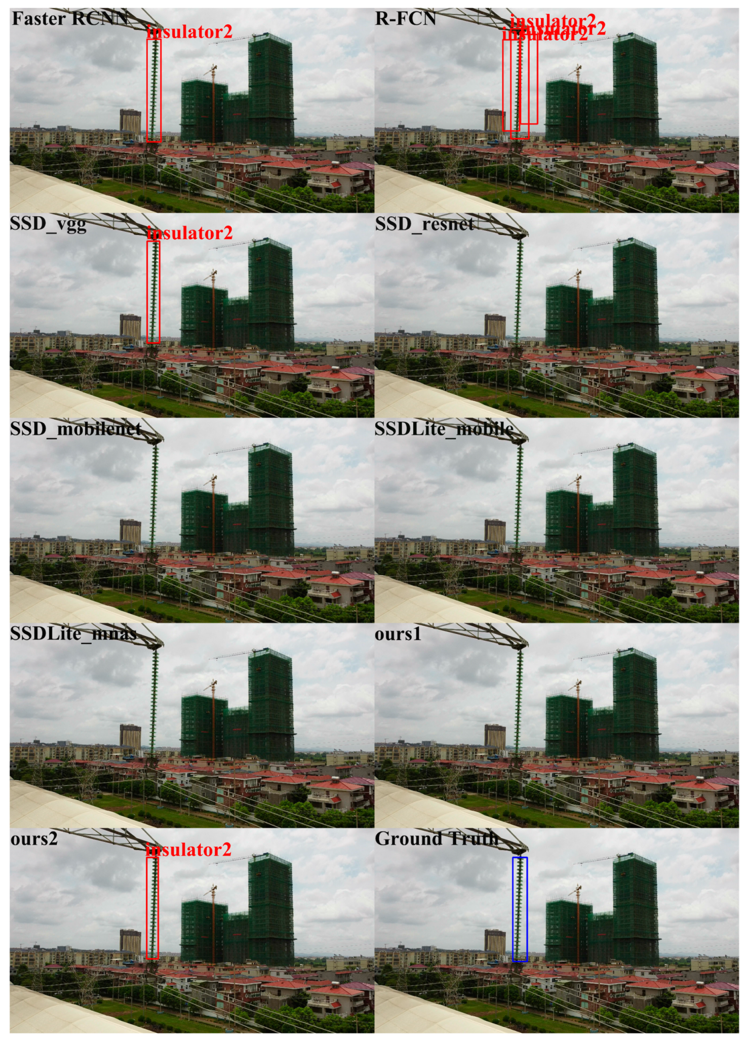
4.5.1. Qualitative Evaluation
4.5.2. Quantitative Evaluation
5. Conclusions
Author Contributions
Funding
Acknowledgments
Conflicts of Interest
References
- Han, S.; Hao, R.; Lee, J. Inspection of insulators on high-voltage power transmission lines. IEEE Trans. Power Deliv. 2009, 24, 2319–2327. [Google Scholar] [CrossRef]
- Katrasnik, J.; Pernus, F.; Likar, B. A survey of mobile robots for distribution power line inspection. IEEE Trans. Power Deliv. 2010, 25, 485–493. [Google Scholar] [CrossRef]
- Li, D.; Wang, X. The future application of transmission line automatic monitoring and deep learning technology based on vision. In Proceedings of the 2019 IEEE 4th International Conference on Cloud Computing and Big Data Analysis (ICCCBDA), Chengdu, China, 12–15 April 2019; pp. 131–137. [Google Scholar]
- Gao, Y.; Song, G.; Li, S.; Zhen, F.; Chen, D.; Song, A. LineSpyX: A power line inspection robot based on digital radiography. IEEE Robot. Autom. Lett. 2020, 5, 4759–4765. [Google Scholar] [CrossRef]
- Zhou, Q.; Zhou, X.-l.; Li, X.-p.; Xiao, J.; Zhou, T.; Wang, C.-j. Mechanical design and research of a novel power lines inspection robot. In Proceedings of the 2016 International Conference on Integrated Circuits and Microsystems (ICICM), Chengdu, China, 23–25 November 2016; pp. 363–366. [Google Scholar]
- Yue, X.; Wang, H.; Yang, Y.; Jiang, Y. Geometric design of an inspection robot for 110kV power transmission lines. In Proceedings of the 2016 4th International Conference on Applied Robotics for the Power Industry (CARPI), Jinan, China, 11–13 October 2016; pp. 1–5. [Google Scholar]
- Mao, T.; Huang, K.; Zeng, X.; Ren, L.; Wang, C.; Li, S.; Zhang, M.; Chen, Y. Development of power transmission line defects diagnosis system for UAV inspection based on binocular depth imaging technology. In Proceedings of the 2019 2nd International Conference on Electrical Materials and Power Equipment (ICEMPE), Guangzhou, China, 7–10 April 2019; pp. 478–481. [Google Scholar]
- Nguyen, V.N.; Jenssen, R.; Roverso, D. Automatic autonomous vision-based power line inspection: A review of current status and the potential role of deep learning. Int. J. Electr. Power Energy Syst. 2018, 99, 107–120. [Google Scholar] [CrossRef]
- Heng, Y.; Tao, G.; Ping, S.; Fengxiang, C.; Wei, W.; Xiaowei, L. Anti-vibration hammer detection in UAV image. In Proceedings of the 2017 2nd International Conference on Power and Renewable Energy (ICPRE), Chengdu, China, 20–23 September 2017; pp. 204–207. [Google Scholar]
- Ren, S.; He, K.; Girshick, R.; Sun, J. Faster R-CNN: Towards real-time object detection with region proposal networks. arXiv 2015, arXiv:1506.01497. [Google Scholar] [CrossRef]
- Chen, H.; He, Z.; Shi, B.; Zhong, T. Research on recognition method of electrical components based on YOLO V3. IEEE Access 2019, 7, 157818–157829. [Google Scholar] [CrossRef]
- Ward, C.M.; Harguess, J.; Crabb, B.; Parameswaran, S. Image quality assessment for determining efficacy and limitations of Super-Resolution Convolutional Neural Network (SRCNN). arXiv 2019, arXiv:1905.05373. [Google Scholar]
- Redmon, J.; Farhadi, A. YOLOv3: An incremental improvement. arXiv 2018, arXiv:1804.02767. [Google Scholar]
- Prates, R.M.; Cruz, R.; Marotta, A.P.; Ramos, R.P.; Filho, E.F.S.; Cardoso, J.S. Insulator visual non-conformity detection in overhead power distribution lines using deep learning. Comput. Electr Eng. 2019, 78, 343–355. [Google Scholar] [CrossRef]
- Simonyan, K.; Zisserman, A. Very deep convolutional networks for large-scale image recognition. arXiv 2015, arXiv:1409.1556. [Google Scholar]
- Jiang, H.; Qiu, X.; Chen, J.; Liu, X.; Miao, X.; Zhuang, S. Insulator fault detection in aerial images based on ensemble learning with multi-level perception. IEEE Access 2019, 7, 61797–61810. [Google Scholar] [CrossRef]
- Howard, A.G.; Zhu, M.; Chen, B.; Kalenichenko, D.; Wang, W.; Weyand, T.; Andreetto, M.; Adam, H. MobileNets: Efficient convolutional neural networks for mobile vision applications. arXiv 2017, arXiv:1704.04861. [Google Scholar]
- Liu, W.; Anguelov, D.; Erhan, D.; Szegedy, C.; Reed, S.E.; Fu, C.Y.; Berg, A.C. SSD: Single Shot MultiBox Detector. arXiv 2015, arXiv:1512.02325. [Google Scholar]
- Hu, L.; Ma, J.; Fang, Y. Defect recognition of insulators on catenary via multi-oriented detection and deep metric learning. In Proceedings of the 2019 Chinese Control Conference (CCC), Guangzhou, China, 27–30 July 2019; pp. 7522–7527. [Google Scholar]
- Han, J.; Yang, Z.; Xu, H.; Hu, G.; Zhang, C.; Li, H.; Lai, S.; Zeng, H. Search like an eagle: A cascaded model for insulator missing faults detection in aerial images. Energies 2020, 13, 713. [Google Scholar] [CrossRef]
- Dai, J.; Li, Y.; He, K.; Sun, J. R-FCN: Object detection via region-based fully convolutional networks. arXiv 2016, arXiv:1605.06409. [Google Scholar]
- Tan, M.; Chen, B.; Pang, R.; Vasudevan, V.; Sandler, M.; Howard, A.; Le, Q.V. MnasNet: Platform-aware neural architecture search for mobile. arXiv 2018, arXiv:1807.11626. [Google Scholar]
- Meng, L.; Peng, Z.; Zhou, J.; Zhang, J.; Lu, Z.; Baumann, A.; Du, Y. Real-time detection of ground objects based on unmanned aerial vehicle remote sensing with deep learning: Application in excavator detection for pipeline safety. Remote Sens. 2020, 12, 182. [Google Scholar] [CrossRef]
- Tijtgat, N.; Van Ranst, W.; Volckaert, B.; Goedemé, T.; De Turck, F. Embedded real-time object detection for a uav warning system. In Proceedings of the 2017 IEEE International Conference on Computer Vision Workshops (ICCVW), Venice, Italy, 22–29 October 2017; pp. 2110–2118. [Google Scholar]
- Deng, J.; Dong, W.; Socher, R.; Li, L.; Li, K.; Fei-Fei, L. ImageNet: A large-scale hierarchical image database. In Proceedings of the 2009 IEEE Conference on Computer Vision and Pattern Recognition, Miami, FL, USA, 20–25 June 2009; pp. 248–255. [Google Scholar]
- Lin, T.-Y.; Dollár, P.; Girshick, R.B.; He, K.; Hariharan, B.; Belongie, S.J. Feature pyramid networks for object detection. arXiv 2016, arXiv:1612.03144. [Google Scholar]
- Kingma, D.P.; Ba, J. Adam: A method for stochastic optimization. arXiv 2015, arXiv:1412.6980. [Google Scholar]
- Everingham, M.; Van Gool, L.; Williams, C.K.I.; Winn, J.; Zisserman, A. The pascal visual object classes (VOC) challenge. Int. J. Comput. Vis. 2010, 88, 303–338. [Google Scholar] [CrossRef]
- Paszke, A.; Gross, S.; Massa, F.; Lerer, A.; Bradbury, J.; Chanan, G.; Killeen, T.; Lin, Z.; Gimelshein, N.; Antiga, L.; et al. PyTorch: An imperative style, high-performance deep learning library. arXiv 2019, arXiv:1912.01703. [Google Scholar]
- Sandler, M.; Howard, A.; Zhu, M.; Zhmoginov, A.; Chen, L. MobileNetV2: Inverted residuals and linear bottlenecks. In Proceedings of the 2018 IEEE/CVF Conference on Computer Vision and Pattern Recognition, Salt Lake City, UT, USA, 18–23 June 2018; pp. 4510–4520. [Google Scholar]
- He, K.; Zhang, X.; Ren, S.; Sun, J. Deep residual learning for image recognition. arXiv 2015, arXiv:1512.03385. [Google Scholar]


| Label | Insulator1 | Insulator2 | Spacer |
|---|---|---|---|
| Object numbers | 1485 | 613 | 199 |
| Simplified Name | Backbone | Main Modules |
|---|---|---|
| Faster R-CNN | ResNet-101 | Faster R-CNN(ResNet-101) 1 |
| R-FCN | ResNet-101 | R-FCN(ResNet-101) |
| SSD_vgg | VGG-16 | SSD(VGG-16) |
| SSD_resnet | ResNet-101 | SSD(ResNet-101) |
| SSD_mobilenet | MobileNet_V2 | SSD(MobileNet_V2) |
| SSDLite_mobile | MobileNet_V2 | SSDLite (MobileNet_V2) |
| SSDLite_mnas | MnasNet | SSDLite (MnasNet) |
| Ours1 | MnasNet | SSD (MnasNet + Feature fusion + Channel plus) 2 |
| Ours2 | MnasNet | SSD (MnasNet + Feature fusion + Channel concatenate) 3 |
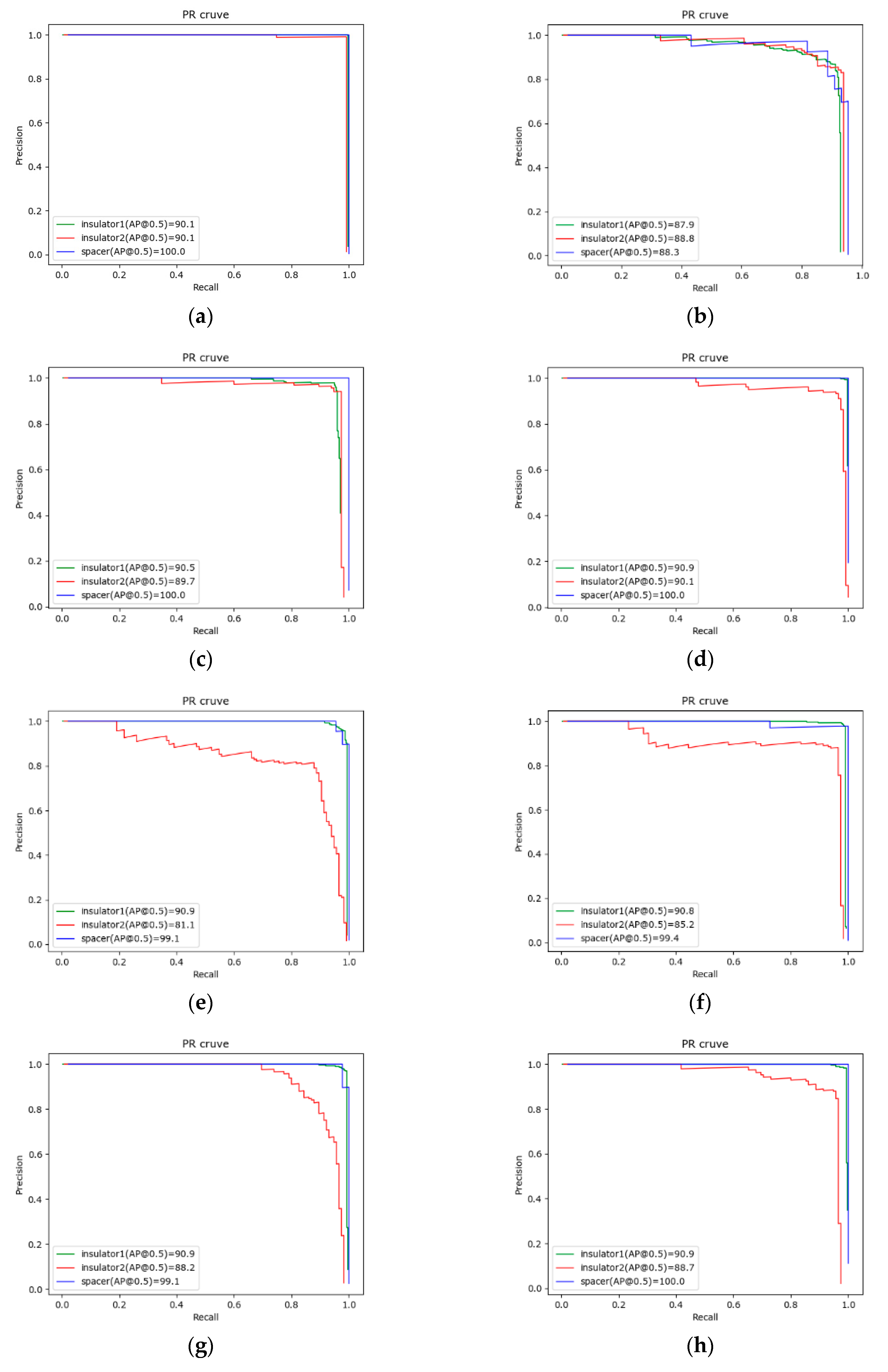
| Method | Insulator1 AP (%) | Insulator2 AP (%) | Spacer AP (%) | mAP (%) |
|---|---|---|---|---|
| Faster R-CNN | 90.1 | 90.1 | 100.0 | 93.4 |
| R-FCN | 87.9 | 88.8 | 88.3 | 88.1 |
| SSD_vgg | 90.5 | 89.7 | 100.0 | 93.4 |
| SSD_resnet | 90.9 | 90.1 | 100.0 | 93.7 |
| SSD_mobilenet | 90.9 | 81.1 | 99.1 | 90.3 |
| SSDLite_mobile | 90.8 | 85.2 | 99.4 | 91.8 |
| SSDLite_mnas | 90.9 | 88.2 | 99.1 | 92.7 |
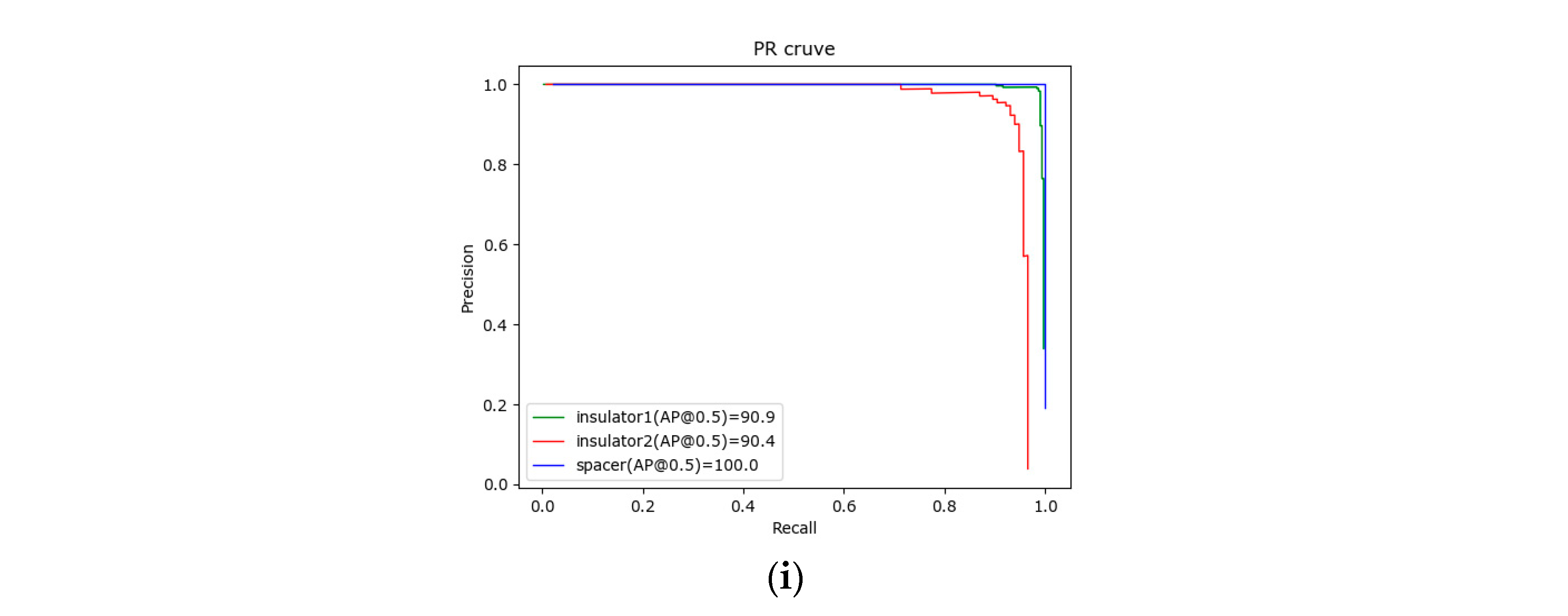
| Ours1 | 90.9 | 88.7 | 100.0 | 93.2 |
| Ours2 | 90.9 | 90.4 | 100.0 | 93.8 |
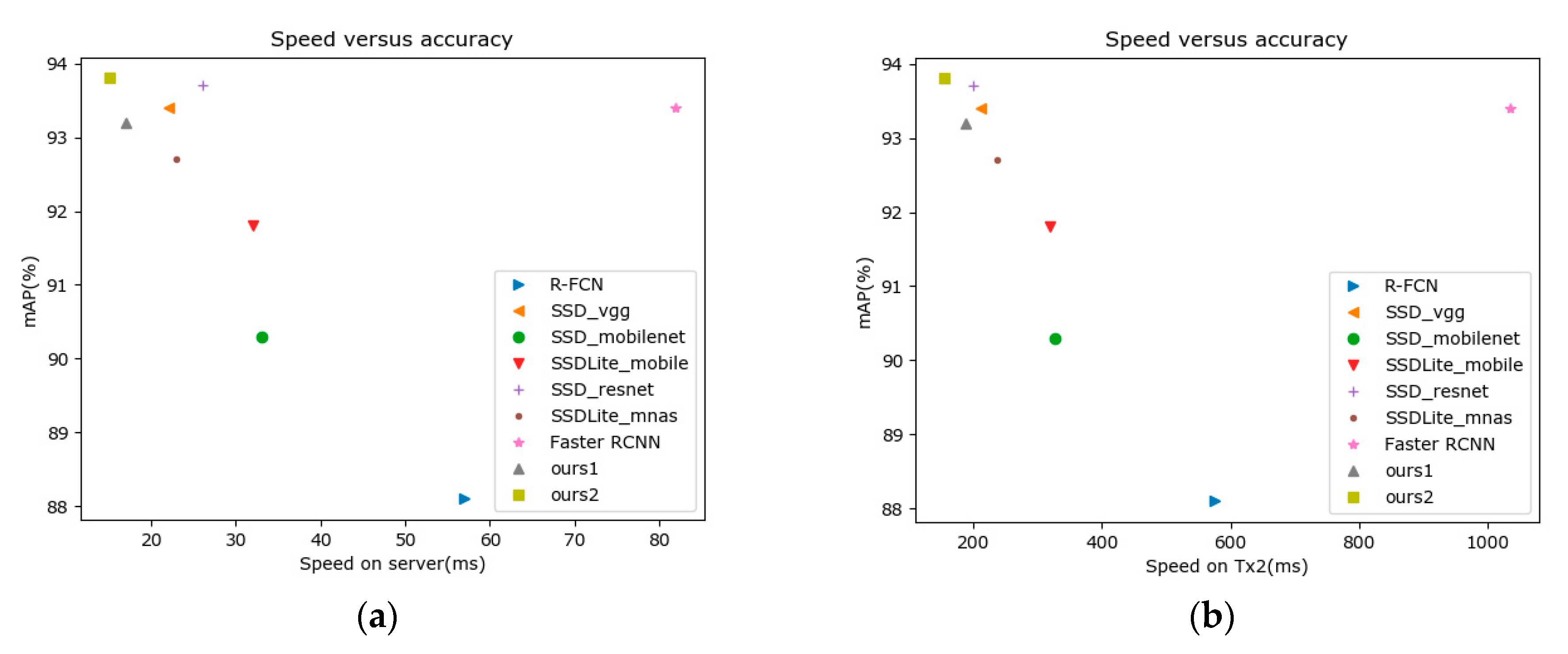
| Method | Model Size (MB) | Server_Time (ms) | TX2_Time (ms) | TX2_Vartime (ms) |
|---|---|---|---|---|
| Faster R-CNN | 360.07 | 82 | 1036 | 40 |
| R-FCN | 383.42 | 57 | 576 | 58 |
| SSD_vgg | 91.62 | 22 | 211 | 66 |
| SSD_resnet | 211.17 | 26 | 200 | 70 |
| SSD_mobilenet | 40.38 | 33 | 327 | 76 |
| SSDLite_mobile | 11.91 | 32 | 320 | 76 |
| SSDLite_mnas | 19.77 | 23 | 238 | 70 |
| Ours1 | 43.58 | 17 | 189 | 54 |
| Ours2 | 43.73 | 15 | 154 | 45 |
| Model | Server (fps) | TX2 (fps) |
|---|---|---|
| Ours1 | 10.64 | 2.79 |
| Ours2 | 36.85 | 8.27 |
Publisher’s Note: MDPI stays neutral with regard to jurisdictional claims in published maps and institutional affiliations. |
© 2020 by the authors. Licensee MDPI, Basel, Switzerland. This article is an open access article distributed under the terms and conditions of the Creative Commons Attribution (CC BY) license (http://creativecommons.org/licenses/by/4.0/).
Share and Cite
Liu, X.; Li, Y.; Shuang, F.; Gao, F.; Zhou, X.; Chen, X. ISSD: Improved SSD for Insulator and Spacer Online Detection Based on UAV System. Sensors 2020, 20, 6961. https://doi.org/10.3390/s20236961
Liu X, Li Y, Shuang F, Gao F, Zhou X, Chen X. ISSD: Improved SSD for Insulator and Spacer Online Detection Based on UAV System. Sensors. 2020; 20(23):6961. https://doi.org/10.3390/s20236961
Chicago/Turabian StyleLiu, Xuan, Yong Li, Feng Shuang, Fang Gao, Xiang Zhou, and Xingzhi Chen. 2020. "ISSD: Improved SSD for Insulator and Spacer Online Detection Based on UAV System" Sensors 20, no. 23: 6961. https://doi.org/10.3390/s20236961
APA StyleLiu, X., Li, Y., Shuang, F., Gao, F., Zhou, X., & Chen, X. (2020). ISSD: Improved SSD for Insulator and Spacer Online Detection Based on UAV System. Sensors, 20(23), 6961. https://doi.org/10.3390/s20236961